A joint approach for reducing eccentricity and spurious gravitational radiation
in binary black hole initial data construction

Abstract

At the beginning of binary black hole simulations, there is a pulse of spurious radiation (or junk radiation) resulting from the initial data not matching astrophysical quasi-equilibrium inspiral exactly. One traditionally waits for the junk radiation to exit the computational domain before taking physical readings, at the expense of throwing away a segment of the evolution, and with the hope that junk radiation exits cleanly. We argue that this hope does not necessarily pan out as junk radiation could excite long-lived constraint violation. Another complication with the initial data is that it contains orbital eccentricity that needs to be removed, usually by evolving the early part of the inspiral multiple times with gradually improved input parameters. We show that this procedure is also adversely impacted by junk radiation. In this paper, we do not attempt to eliminate junk radiation directly, but instead tackle the much simpler problem of ameliorating its long-lasting effects. We report on the success of a method that achieves this goal by combining the removal of junk radiation and eccentricity into a single procedure. Namely we periodically stop a low resolution simulation; take the numerically evolved metric data and overlay it with eccentricity adjustments; run it through initial data solver (i.e. the solver receives as free data the numerical output of the previous iteration); restart the simulation; repeat until eccentricity becomes sufficiently low, and then launch the high resolution “production run” simulation. This approach has the following benefits: (1) We do not have to contend with the influence of junk radiation on eccentricity measurements for later iterations of the eccentricity reduction procedure. (2) We re-enforce constraints every time initial data solver is invoked, removing the constraint violation excited by junk radiation previously. (3) The wasted simulation segment associated with the junk radiation’s evolution is absorbed into the eccentricity reduction iterations. Furthermore, (1) and (2) together allow us to carry out our joint-elimination procedure at low resolution, even when the subsequent “production run” is intended as a high resolution simulation.

I Introduction

Binary black hole coalescences constitute one of the most promising sources for the gravitational wave detectors such as Advanced LIGO Harry (2010) (for the LIGO Scientific Collaboration), Virgo The Virgo Collaboration (2009, 2012) and KAGRA Somiya (2012). In order to achieve a detection, we need numerical simulations to calibrate and validate the template bank of waveforms.

When we prepare the initial data to be used in such a binary black hole simulation, we could not obtain an exact snapshot of a quasi-equilibrium inspiral. Once the simulation begins, the spacetime relaxes into a quasi-equilibrium configuration with the mismatch radiating away as a pulse of spurious or “junk” radiation (JR). JR, therefore, can be thought of as the gravitational perturbation one needs to add to the quasi-equilibrium solution in order to obtain the solution used as numerical initial data. Part of this perturbation will propagate outwards immediately as outgoing gravitational radiation. Another part corresponds to an ingoing radiation that results in a small but long lasting transient Bishop et al. (2011). Yet another part will fall onto the black holes, exciting quasi-normal ringing which, in turn, will result in outgoing gravitational waves of much higher frequency than those generated by the orbital motion of the binary Lovelace (2009); Boyle et al. (2007).

Resolving the highest frequency components of JR, although possible, is not practical as our numerical grid is tuned for resolving the quasi-equilibrium system, where all short ($\approx 1M$) length-scale features are in the immediate neighborhood of the binary, while the grid in the outer regions is built to resolve wave propagation on much larger ($\approx 100M$) length-scales. The alternative approach had been to just accept the fact JR is not resolved and wait for it to leave the computational domain Lovelace (2009). The result is that the JR may morph into constraint violation (CV) that can alter the physical properties of the system (individual masses and spins, orbital parameters), and degrade the accuracy of the simulation for longer than one light-crossing time of the computational domain.

Another complication with constructing initial data is the astrophysically motivated need for low orbital eccentricity (OE). Given that gravitational radiation tends to circularize binary orbits Peters and Mathews (1963); Peters (1964); Postnov and Yungelson (2005), it is expected that for binaries born from stellar evolution, rather than e.g. dynamical capture scenarios East et al. (2013), little OE would remain by the time the system enters into the sensitive band of the next generation of ground-based gravitational wave detectors. It is therefore desirable to remove OE in simulations meant to generate waveforms for the template banks of these detectors. This entails evolving the simulation for a small number of orbits and reading off the oscillation in the orbital angular velocity of the black holes. Then this data is used to generate an improved set of initial data parameters. Such a procedure is repeated a number of times until OE reduces to an acceptable level. Junk radiation complicates this procedure by introducing a long-lasting disturbance into the eccentricity measurement of the binary.

In this paper, we aim to reduce such long-lasting secondary effects created by JR. To this end, we simply modify the traditional approach where one waits for the JR to exit the outer boundary before taking physical readings . In our approach, at the end of each eccentricity reduction iteration, we make use of the numerically evolved metric data, apply adjustments on the black holes’ velocities, and then re-solve the constraints before continuing on, rather than adjusting the initial data parameters and starting the run from the same point as in the initial iteration.

After the initial iteration of this “stop-and-go” operation, the JR will have passed through the computational domain. Furthermore, by invoking the initial data solver, we not only blend in the velocity adjustments, but also remove CV built up previously. In other words, we resolve the issue that JR does not exit cleanly. For later iterations, the eccentricity measurement of the binary is no longer perturbed by the JR, allowing for a more robust eccentricity reduction procedure. After a few iterations, we would have converged onto a snapshot of an astrophysically realistic inspiral that has reduced JR, OE, as well as CV, which can be used as the initial data for a high resolution “production run” simulation. From this perspective, we have jointly eliminated OE and the impact of JR with a numerical process. We thus refer to this collection of “stop-and-go” iterations as the “joint-elimination” approach.

It is worth mentioning that we regard our method as being complementary to the analytical approach, where one targets the JR itself by obtaining a more realistic initial data through adding more analytical components into it Johnson-McDaniel et al. (2009), such as wave content Kelly et al. (2007), tidal deformations, or allowing for conformally curved initial data Johnson-McDaniel et al. (2009); Lovelace (2009). These algorithms are aimed at reducing the JR in what we refer to as the initial iteration (to be followed by first, second etc iterations) of the joint-elimination approach. The resulting quasi-equilibrium system has a better chance of closely matching the desired physical parameters. However, inherent to these analytic approaches, one must employ some sort of blending, truncated expansion, etc. The resulting initial data will be different from the quasi-equilibrium system, and will generate some amount of JR. Our approach then takes whatever outcome is available from the analytical procedures, evolve it through the JR phase, and construct a subsequent evolution that is now based on the numerically achieved quasi-equilibrium solution.

Our study is carried out with the Spectral Einstein Code (SpEC) SXS , a pseudospectral code that solves a first differential order form of the generalized harmonic formulation of Einstein’s equations Lindblom et al. (2006a); Friedrich (1985); Garfinkle (2002); Pretorius (2005). The overall domain of evolution is divided into the so-called “subdomains” that are simply spherical shells near the excision boundaries and in the gravitational wave zone, and are more complicated shapes in the inner regions M. A. Scheel, M. Boyle, T. Chu, L. E. Kidder, K. D. Matthews and H. P. Pfeiffer (2009); Szilagyi et al. (2009).

We begin by summarizing some useful background information in Sec. II, before moving on to elaborate on the junk radiation’s long-lasting impacts in Sec. III. In Sec. IV, we describe the joint-elimination procedure, and then in Sec. V, we demonstrate its effectiveness and advantages.

In the formulae below, the early part of the Latin alphabet denotes spacetime indices that run from 0 to 3, while the mid part of the Latin alphabet denotes spatial indices (from 1 to 3). Bold face letters represent tensors or vectors. Unless stated otherwise, the figures depict the inspiral stage of an equal-mass nonspinning black hole binary simulation (referred to as the “standard example”), beginning from conformally flat initial data with an initial coordinate separation of $15$M (M being the total mass). This simulation is carried out on the overlapping subdomain decomposition of M. A. Scheel, M. Boyle, T. Chu, L. E. Kidder, K. D. Matthews and H. P. Pfeiffer (2009); Szilagyi et al. (2009), at the lowest resolution typically used in a convergence study.

II Preliminaries

In this section, we review some of the formalisms used in initial data construction, eccentricity reduction and spacetime curvature visualization. Our joint-elimination procedure will use a variant of the methods summarized here. The adaptations will be summarized in Sec. IV.

II.1 Vacuum initial value problem

In the standard $3+1$ form of Einstein’s equations Arnowitt et al. (1962); York, Jr. (1979), the metric is written as

$$ds^{2}=-N^{2}dt^{2}+g_{ij}\left(dx^{i}+N^{i}dt\right)\left(dx^{j}+N^{j}dt\right)$$ (1)

where $N$ is the lapse, $N^{i}$ is the shift, and $g_{ij}$ is the three metric on a constant $t$ hypersurface.

The extrinsic curvature of that hypersurface is given by

$${\bf K}=-\frac{1}{2}\mathbb{P}\mathcal{L}_{{\bf n}}{}^{(4)}{\bf g}$$ (2)

where ${}^{(4)}\bf{g}$ is the spacetime metric, $\mathcal{L}_{{\bf n}}$ is the Lie derivative along the unit normal to the hypersurface, and $\mathbb{P}$ is the projection operator into the hypersurface. The definition Eq. (2) leads to

$$\partial_{t}g_{ij}=-2NK_{ij}+\nabla_{i}N_{j}+\nabla_{j}N_{i},$$ (3)

so $K_{ij}$ gives the time derivative of $g_{ij}$ aside from a shift correction, and constitutes the central piece in the Arnowitt-Deser-Misner canonical momentum Arnowitt et al. (1962)

$$\pi^{ij}=\sqrt{g}\left(K^{ij}-Kg^{ij}\right).$$ (4)

Specifying $g_{ij}$ and $K_{ij}$ then amounts to pinning down the initial state in phase space, or in other words providing the initial data. In addition, one should also specify the gauge choice by fixing the initial values for lapse $N$ and shift $N^{i}$.

The initial data is not arbitrary. It has to satisfy the Hamiltonian and momentum constraints

$$R+K^{2}-K_{ij}K^{ij} = 0,$$ (5)

$$\nabla_{j}\left(K^{ij}-g^{ij}K\right) = 0,$$ (6)

where $\nabla_{j}$ is the covariant derivative on the spatial hypersurface, and $R$ is the trace of the spatial Ricci tensor. These constraints represent the condition that $K_{ij}$ and $g_{ij}$ are consistent with being associated with a slice of a vacuum spacetime. In a geometrical sense these constraints enforce that the spatial surface with prescribed $K_{ij}$ and $g_{ij}$ can indeed be immersed into a four dimensional Ricci-flat ambient spacetime.

Constraint satisfying initial data construction is done by designating a set of functions as freely specifiable while leaving the rest determined by the constraint equations. We have one scalar and one vector equation in Eqs. (5) and (6) respectively, so we should leave one scalar plus one vector quantity indeterminate. We assign them to intrinsic metric $g_{ij}$ and extrinsic curvature $K_{ij}$ respectively, and choose the quantities that the constraint equations depend on sensitively. Following the approach of the extended conformal thin sandwich formalism (XCTS) York (1999); Pfeiffer and York (2003), we define

$$g_{ij}=\psi^{4}\tilde{g}_{ij}.$$ (7)

We specify the conformal spatial metric $\tilde{g}_{ij}$ by hand and solve for the conformal factor $\psi$ using essentially the Hamiltonian constraint Eq. (5). We will denote with a tilde quantities associated with the conformal metric. For the momentum constraint Eq. (6), we first decompose extrinsic curvature to its trace (i.e. mean curvature) and the transverse traceless and longitudinal traceless parts

$$K^{ij}=\frac{1}{3}g^{ij}K+M^{ij}+\frac{1}{2N}(\mathbb{L}V)^{ij}\left(\equiv\frac{1}{3}g^{ij}K+A^{ij}\right)$$ (8)

that have the following conformal counterparts

$$\tilde{K} = K,\quad\tilde{M}^{ij}=\psi^{10}M^{ij},$$

$$\quad(\tilde{\mathbb{L}}\tilde{V})^{ij} = \psi^{4}(\mathbb{L}V)^{ij},\quad\tilde{A}_{ij}=\psi^{2}A_{ij}.$$ (9)

The longitudinal operator is defined as

$$(\mathbb{L}V)^{ij}=2\nabla^{(i}V^{j)}-\frac{2}{3}g^{ij}\nabla_{k}V^{k},$$ (10)

and $V^{i}$ can serve as the indeterminate vector field. Comparing Eq. (8) with Eq. (3), we are not surprised to find that when the shift gauge condition is set to $N^{i}=V^{i}$, the conformal $\tilde{M}_{ij}$ simply becomes the (lapse weighted) trace-free part of the time derivative of the conformal metric, which we denote as $\tilde{u}_{ij}$. Under this particular gauge fixing, momentum constraint takes on the pretense of an equation for shift (with some $\psi$ coupled in), even though it is really solving for extrinsic curvature.

We can now rewrite the Hamiltonian and momentum constraints as a pair of coupled elliptic equations for $\psi$ and $N^{i}$. With XCTS, one also sets the lapse gauge condition by specifying $\partial_{t}\tilde{K}$, which translates into an equation for the conformal lapse $\tilde{N}$ Pfeiffer and York (2003); Smarr and York (1978); Wilson and Mathews (1989). The combined system of equations is then

$$\tilde{\nabla}^{2}\psi-\frac{1}{8}\psi\tilde{R}-\frac{1}{12}K^{2}\psi^{5}+\frac{1}{8}\tilde{A}_{ij}\tilde{A}^{ij}\psi^{-7} = 0,$$ (11)

$$\tilde{\nabla}_{j}\left(\frac{1}{2\tilde{N}}(\tilde{\mathbb{L}}\tilde{N})^{ij}\right)-\frac{2}{3}\psi^{6}\tilde{\nabla}^{i}K-\tilde{\nabla}_{j}\left(\frac{\tilde{u}^{ij}}{2\tilde{N}}\right) = 0,$$ (12)

$$\tilde{\nabla}^{2}\left(\tilde{N}\psi^{7}\right)-\left(\tilde{N}\psi^{7}\right)\left[\frac{\tilde{R}}{8}+\frac{5}{12}K^{4}\psi^{4}+\frac{7}{8}\psi^{-8}\tilde{A}^{ij}\tilde{A}_{ij}\right] = -\psi^{5}\left(\partial_{t}K-N^{k}\partial_{k}K\right),$$ (13)

where $\tilde{N}=\psi^{-6}N$. We solve these equations with a multidomain spectral elliptic partial differential equation solver described in Pfeiffer et al. (2003). The pre-determined free-data are the conformal metric $\tilde{g}_{ij}$, the trace-removed part of its time derivative $\tilde{u}_{ij}$, the mean curvature $K$ and its time derivative $\partial_{t}K$. Generating realistic initial data means providing better values for these quantities.

In order to provide sensible free-data, it is convenient to go into a co-rotating frame where the black holes are pinned down at fixed spatial coordinates. There, one can impose the quasi-stationary conditions $\tilde{u}_{ij}=0$ and $\partial_{t}K=0$. The remaining free-data that do not involve time derivatives can be either $\tilde{g}_{ij}=\eta_{ij}$ ($\bf{\eta}$ being the Minkowski spatial metric) and $K=0$ in the conformally flat case, or, for the superposed Kerr-Schild case Lovelace (2009) (more conducive to high spins), a combination of Kerr-Schild black holes inside Gaussian envelopes

$$\tilde{g}_{ij} = \eta_{ij}+\sum_{a=1}^{2}e^{-r_{a}^{2}/\omega_{a}^{2}}(g_{ij}^{a}-\eta_{ij})$$ (14)

$$K = \sum_{a=1}^{2}e^{-r_{a}^{2}/\omega_{a}^{2}}K_{a}$$ (15)

where $g^{a}$ and $K_{a}$ are spatial metric and mean curvature of spinning Kerr-Schild black holes.

The boundary conditions on the unknown variables are also important, as for example in the conformally flat case, the presence and properties of the black holes are completely fixed by the boundary conditions. The shift condition on the excision boundaries in the co-rotating frame is

$$N^{i}=Ns^{i}+N^{i}_{\parallel}$$ (16)

where $s^{i}$ is normal to the boundaries and $N^{i}_{\parallel}$ tangential to it, giving the spin of the black holes. There is no component directly corresponding to the orbital motion of the black holes. That piece of information enters through the boundary condition at spatial infinity $r\rightarrow\infty$ ($r$ is the magnitude of the location vector ${\bf r}$)

$$N^{i}=\xi^{i}\equiv({\bf\Omega}_{0}\times{\bf r})^{i}$$ (17)

After solving for $(\psi_{\text{co}},N_{\text{co}},N_{\text{co}}^{i})$ in the co-rotating frame, translating into the inertial frame solution $(\psi_{\text{in}},N_{\text{in}},N_{\text{in}}^{i})$ is straightforward. It turns out that since $\mathbb{L}{\bf\xi}=0$ Pfeiffer et al. (2007), we have that, provided mean curvature $K$ vanishes, the quantities

$$\psi_{\text{in}}=\psi_{\text{co}},\quad N^{i}_{\text{in}}=N^{i}_{\text{co}},\quad N_{\text{in}}^{i}=N^{i}_{\text{co}}-\xi^{i},$$ (18)

would satisfy the XCTS equations with the inertial frame boundary conditions of

$$N^{i}=Ns^{i}-\xi^{i}+N^{i}_{\parallel}$$ (19)

on the excision boundaries, as well as $N^{i}=0$ at $r\rightarrow\infty$. For the boundary conditions on $\psi$ and $N$, and a more thorough introduction to XCTS formalism, see e.g. Pfeiffer et al. (2007).

II.2 A recursive eccentricity reduction procedure

As discussed in Sec. I, binary black hole initial data construction usually include an eccentricity reduction stage. The method we summarize here is a recursive procedure proposed and developed in Pfeiffer et al. (2007); Boyle et al. (2007); Tichy and Marronetti (2010); Buonanno et al. (2011), whereby initial data are evolved for two to three orbits, before an analysis of the orbit in terms of the separation $s$ between the black hole apparent horizons, or instantaneous angular velocity $\omega$, is carried out to generate an improved set of initial parameters to be used in the next iteration.

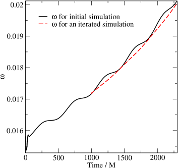
Figure 1: The solid black curve represents the evolution of $\omega$ in the standard example simulation. The wobbles signify the presence of eccentricity. For comparison, we also display as a dashed red curve the $\omega(t)$ for this simulation after one stop-and-go operation described in Sec. IV, which contains an eccentricity suppression step.

Orbital eccentricity manifests itself as an oscillation in $ds/dt$ or $d\omega/dt$ with a period close to the orbital period (but does not need to be exactly equal when periastron advances are present Buonanno et al. (2011)). To separate this oscillation from the smooth decline of orbital separation (the “inspiral”), which is equivalently represented by an increase of orbital frequency $\omega$ (see Fig. 1), the time derivative $d\omega/dt$ (see Ref. Buonanno et al. (2011) for a discussion on the advantage of using $d\omega/dt$ over $ds/dt$) is fitted to a functional form Pfeiffer et al. (2007); Buonanno et al. (2011)

$$\frac{d\omega}{dt} = A_{0}(T-t)^{-11/8}+A_{1}(T-t)^{-13/8}$$ (20)

$$+B\cos(\omega t+\phi+\nu t^{2})$$

by varying parameters $(T,A_{0},A_{1},B,\phi,\nu)$. The first two terms constitute the orbital decay, and the last one is the oscillation due to eccentricity.

From the fitting result, one can calculate the eccentricity estimate

$$e=\frac{B}{2\Omega_{0}\omega},$$ (21)

where $\Omega_{0}$ is the initial angular frequency. We can then calculate how much tangential and radial velocities need to be added onto the black holes in order to drive $e$ to zero. An initial radial velocity can be given to the black holes by changing the boundary condition Eq. (19) on the excision surfaces in the inertial frame to

$$N^{i}=Ns^{i}-\xi_{\rm rad}^{i}+N^{i}_{\parallel},$$ (22)

where

$$\xi_{\rm rad}^{i}\equiv({\bf\Omega}_{0}\times{\bf r})^{i}+\dot{a}_{0}r^{i}.$$ (23)

The formulae (Eqs. (74) and (78) of Buonanno et al. (2011))

$$\delta\Omega_{0}=-\frac{B}{4\Omega_{0}}\sin\phi,\quad\delta\dot{a}_{0}=\frac{B}{2\Omega_{0}}\cos\phi$$ (24)

then provide the adjustments to the orbital angular frequency $\Omega_{0}$ and expansion factor $\dot{a}_{0}$ in Eq. (23), to be used for initial data construction in the next iteration. Note this is not a simple change of gauge into one where the orbit looks superficially circular, but instead a genuine change to physics because the extrinsic curvature is also updated according to Eq. (8).

II.3 Visualizing curvature

In order to study the anatomy of junk radiation, it is beneficial to be able to see the curvature structure within the bulk of spatial slices. To this end, we construct visualization tools based on gauge invariant contractions Carminati and McLenaghan (1991)

$$I=\Psi_{4}\Psi_{0}-4\Psi_{1}\Psi_{3}+3\Psi_{2}^{2},\quad J=\left|\begin{array}[]{ccc}\Psi_{4}&\Psi_{3}&\Psi_{2}\\ \Psi_{3}&\Psi_{2}&\Psi_{1}\\ \Psi_{2}&\Psi_{1}&\Psi_{0}\end{array}\right|,$$ (25)

of the Weyl tensor $C_{abcd}$, where $\Psi^{\prime}s$ are the Newman-Penrose scalars

$$\Psi_{0} = -C_{abcd}l^{a}m^{b}l^{c}m^{d},$$ (26)

$$\Psi_{1} = -C_{abcd}l^{a}n^{b}l^{c}m^{d},$$ (27)

$$\Psi_{2} = -C_{abcd}l^{a}m^{b}\overline{m}^{c}n^{d},$$ (28)

$$\Psi_{3} = -C_{abcd}l^{a}n^{b}\overline{m}^{c}n^{d},$$ (29)

$$\Psi_{4} = -C_{abcd}n^{a}\overline{m}^{b}n^{c}\overline{m}^{d}.$$ (30)

extracted on any Newman-Penrose null tetrad $\{l_{a},n_{a},m_{a},\overline{m}_{a}\}$ that consists of a pair of null vectors $({\bf l,n})$ and a complex conjugate pair of complex vectors $({\bf m,\overline{m}})$, satisfying normalization conditions such that the spacetime metric takes the standard form of

$$\begin{pmatrix}0&-1&0&0\\ -1&0&0&0\\ 0&0&0&1\\ 0&0&1&0\end{pmatrix}$$ (31)

on that tetrad basis. The expression

$$\Psi^{t}_{2}=-\frac{1}{2}\left(P+\frac{I}{3P}\right)$$ (32)

where

$$P=\left[J+\sqrt{J^{2}-(I/3)^{3}}\right]^{1/3},$$ (33)

then gives the Coulomb background part of the Weyl tensor Szekeres (1965); Baker and Campanelli (2000). Defining a pair of geometrical coordinates by Zhang et al. (2011)

$$\Psi^{t}_{2}=M(\rho^{t})^{3},\quad\rho^{t}=\frac{1}{r^{t}-ia\cos(\theta^{t})},$$ (34)

we obtain a gauge invariant depiction of the structure of the Coulomb background in the form of $(r^{t},\theta^{t})$ contours. For example, in the Kerr limit $(r^{t},\theta^{t})$ become the Boyer-Lindquist coordinates whose contours, when plotted in Kerr-Schild slicing and spatial coordinates, are asymptotically simple spherical shells and cones (see Fig. 1 in Zhang et al. (2011)).

III Some features of junk radiation

III.1 A quadrupolar component of junk radiation

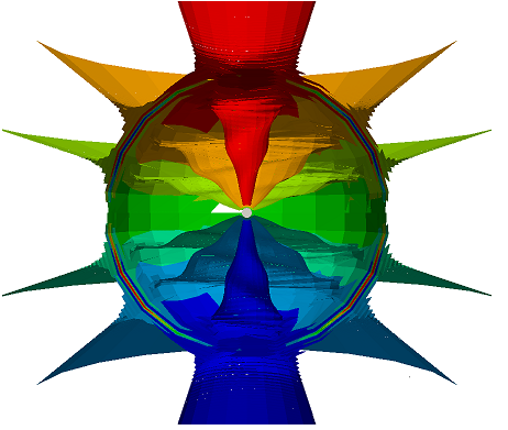
Figure 2: Reproduced from Zhang et al. (2011). Visualization of junk radiation as the boundary between unrealistic and realistic multipole structures in $\theta^{t}$ contours.

The ability to see the curvature structure is useful for visualizing JR because it marks the boundary between the regions containing unrealistic initial data and the post-JR realistic data. As can be seen in the $\theta^{t}$ contours of Fig. 2 (shown originally in Zhang et al. (2011)), the region behind JR shows the signature spiral staircase pattern (see Fig. 2 in Zhang et al. (2011)) generated by a rotating mass quadrupole. Essentially the quadrupolar moment squashes the cones of $\theta^{t}$ contour, and the rotation in this moment causes the squashing direction to vary depending on the distance to the source region, thus forming a twisting pattern. On the other hand, the region ahead of JR does not contain the influence of the rotating quadrupolar moment, because the superposed Kerr-Schild initial data being plotted does not correctly account for inspiral history. Such an absence of past history is more typically seen in Newtonian instantaneous action theories, and is a valid approximation in our general relativistic context only when we are close to the black holes, where the time retardation effect is insignificant.

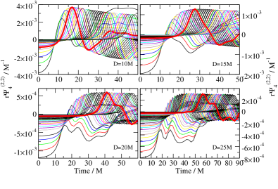
Figure 3: The $(l=2,m=2)$ mode of $r\Psi_{4}$ waveform extracted at various coordinate radii $r_{\text{ex}}\geq D+1$M, with the thick red curve representing $r_{\text{ex}}\approx\lambdabar$. Curves with peaks further to the right correspond to larger $r_{\text{ex}}$. The four panels describe simulations that are similar to the standard example but with initial separations of $D=10$M, $15$M, $20$M and $25$M, and corresponding $\lambdabar=15.8$M, $29.0$M, $44.7$M and $62.5$M.

To see whether this missing inspiral history represents the dominant omission in initial data, we turn to the spatial distribution of JR magnitude. We begin by noting that an approximate limit beyond which the instantaneous initial data becomes invalid is given by

$$r\gtrsim\lambdabar=\frac{1}{2}\sqrt{\frac{D^{3}}{M}}$$ (35)

in Ref. Nichols et al. (2011) (see Figures 18 and 19 in that paper), where $\lambdabar$ is the reduced gravitational wavelength with $D$ being the initial binary separation and $M$ the total mass. The contribution from missing inspiral history should begin picking up magnitude after JR reaches $r\approx\lambdabar$, but those from near-zone dynamics should begin tapering off (i.e. $r\Psi_{4}$ flattens) at this demarcation line between the near and transition zones Nichols et al. (2011). We then carry out equal-mass nonspinning simulations with initial separations of $D=10$M, $15$M, $20$M and $25$M, and corresponding $\lambdabar=15.8$M, $29.0$M, $44.7$M and $62.5$M. In Fig. 3, we plot the $(l=2,m=2)$ mode of $r\Psi_{4}$ waveform in these simulations extracted at various coordinate radii $r_{\text{ex}}\geq D+1$M, with the thick red curve corresponding to $r_{\text{ex}}\approx\lambdabar$. We concentrate on the early part of the waveforms and examine whether magnitude of the junk radiation rose significantly for those extraction radii satisfying $r_{\text{ex}}>\lambdabar$ (these are the curves with peaks to the right of the thick red curve). The absence of this growth in JR magnitude in Fig. 3 then suggests that the missing inspiral history is unlikely the most significant source of JR.

III.2 Excitation of constraint violation

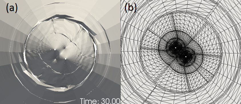
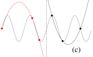
Figure 4: (a) Equatorial plane slice of the computational domain in the standard example simulation (but with a non-overlapping subdomain decomposition for better visual clarity), warped into the paper according to $r^{t}$ value. The impact of JR on the subdomain boundaries is to tear them open in the fashion depicted in Panel (c). (b) The subdomain boundaries in (a) are shown as dense concentration of lines in this panel. Their location matches the tearing. (c) A stylized demonstration that under-resolved high frequency JR (denoted by blue sinusoidal curve) causes mismatch of data at subdomain boundary (vertical dashed line). Red and black curves are the representations of the JR in the left and right subdomains respectively, constructed from sampling at the under-populated red and black dots.

By visualizing $r^{t}$, one can also learn interesting features of JR with regard to generating constraint violation. The high frequency JR requires finer grids to resolve, which would cause the time step size to also drop according to Courant limit. This is a very high computational cost, so even for simulations equipped with Adaptive Mesh Refinement Lovelace et al. (2011) (our simple standard example isn’t), the refinement is left off in the gravitational wave zone until the JR has left the computational domain. The result is that JR is under-resolved in all or some of the regions, and turns into constraint violating modes that degrade the accuracy of the output.

One place where the creation of constraint violation is particularly visible is at subdomain boundaries. The penalty method Hesthaven (1997, 1999, 2000); Gottlieb and Hesthaven (2001) adopted by some pseudospectral codes such as SpEC does not force the values of data across the subdomain boundaries to match up exactly, so the high frequency under-resolved JR will tear the boundary open, as is graphically explained in Fig. 4 (c) and demonstrated for an actual simulation in Fig. 4 (a), creating discontinuities and thus constraint violation. Eventually the gap at the boundaries will be closed by the penalty, but constraint violation will generally take longer to damp out.

To demonstrate this relative longevity of constraint violation, we plot, in Fig. 5, the $(l=2,m=2)$ mode gravitational wave $r\Psi_{4}$ for the standard equal-mass non-spinning binary simulation extracted at a sphere $110$M from the coordinate center, as well as the $L_{2}$ norm of the constraint violation in a spherical shell subdomain (extending radially from $99$M to $120$M) surrounding that extraction radius. The constraint violation is measured using the Generalized Harmonic Constraint Energy (GhCe) defined in Lindblom et al. (2006b), which includes modes that violate the generalized harmonic gauge constraints, and those secondary constraints introduced when reducing the evolution equations to first order. The $L_{2}$ norm is defined as

$$L_{2}(\text{GhCe})=\sqrt{\sum_{q=1}^{N}\frac{\text{GhCe}({\bf x}_{q})^{2}}{N}}$$ (36)

where ${\bf x}_{q}$ are the spectral collocation points and $N$ their total population.

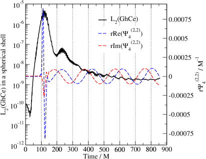
Figure 5: The constraint violation and waveform near the start of the standard example simulation. The dashed blue and red lines are $r$ times the real and imaginary parts of the $(l=2,m=2)$ mode of $\Psi_{4}$ wave extracted at a coordinate radius of $110$M. The Solid black curve is the $L_{2}$ norm of the constraint energy GhCe within a spherical shell extending radially from $99$M to $120$M (i.e. containing the wave extraction sphere). Comparing these curves, we see that constraint violation remains elevated for a long time after the junk radiation (the sharp features at the beginning of the waveforms) has already passed through the spherical shell.

From Fig. 5, we see that the junk radiation may excite the constraint violation by many orders of magnitude, which remains elevated long after $t\approx 150$M when according to the $r\Psi_{4}$ curves, one would estimate the JR to have exited the spherical shell under consideration. Indeed even the JR itself may have a tail (invisible in $r\Psi_{4}$ but possibly connected to the oscillations in $L_{2}(\text{GhCe})$) resulting from new JR being excited by the primary one, which can initially travel back towards the origin Boyle et al. (2007). A hint of this is shown in Refs. Boyle et al. (2007); M. A. Scheel, M. Boyle, T. Chu, L. E. Kidder, K. D. Matthews and H. P. Pfeiffer (2009) where a secondary pulse of JR has been observed to last for two additional light-crossing times after the primary JR has already exited.

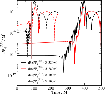
Figure 6: The junk radiation in the $r\Psi_{4}$ waveforms extracted at coordinate radii $r_{\text{ex}}=100$M and $380$M, denoted by dashed and solid curves respectively. The expected arrival times, as $r_{\text{ex}}$ minus black hole initial separation, are plotted as vertical lines. The peak of JR stay relatively consistent in its time lag from the expected arrival time, but the superluminally moving leading edge runs further ahead in the case where $r_{\text{ex}}$ is larger.

Before moving on, we note that the reason constraint violation starts rising before the expected JR arrival time of $99\text{M}-15\text{M}=84$M is because the JR tends to widen over time when under-resolved. Namely, upon entering into a new subdomain, JR corrupts the spectral representation of the entire subdomain simultaneously, thus appears to teleport instantaneously to the other side of that subdomain, giving the appearance of a superluminally moving leading edge. This effect is demonstrated in Fig. 6.

III.3 Impact on eccentricity estimate

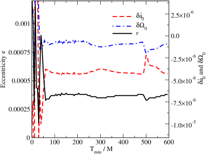
Figure 7: The dependence on $T_{\text{min}}$ of eccentricity $e$ (left vertical axis) estimated by Eq. (21) and $(\delta\dot{a}_{0},\delta\Omega_{0})$ (right vertical axis) suggested by Eq. (24), for the first traditional approach eccentricity reduction iteration (see Sec. V below) of the standard example simulation.

Junk radiation complicates the eccentricity removal procedure by introducing high frequency and large amplitude components into $d\omega/dt$, making fitting by Eq. (20) difficult. Therefore one has to wait for the transient effects created by junk radiation to die down before a fitting can be made. One does this by specifying a $T_{\text{min}}$, while the maximum time in the fitting interval $T_{\text{max}}$ is determined accordingly as $T_{\text{min}}+5\pi/\Omega_{0}$, i.e. fitting is done with just over two orbits after $T_{\text{min}}$.

The dependence on $T_{\text{min}}$ is shown in Fig. 7 for the standard example simulation. We once again observe a long-lasting impact of JR that prevents $\delta\Omega_{0}$ and $\delta\dot{a}_{0}$ estimates from settling down quickly. Aside from the ingoing and secondary JR and the lingering constraint violation (which is less severe for the subdomains close to the black holes that have higher resolution), we have a new complication in this case. We first recall that although the data being evolved corresponds to that measured in an “inertial frame” whose coordinates $\{x_{I}\}$ correspond to inertial observers asymptotically, the spectral computation is done on a co-moving “grid” coordinate system $\{x_{G}\}$ in which black holes remain undeformed and located at fixed positions Scheel et al. (2006). A feedback control system Hemberger et al. (2013) is used to connect the two coordinate systems by essentially tracking the motion of the black holes in the inertial frame. One parameter in this control system that tracks the orbital rotation of the black holes is used as the $\omega$ variable appearing in Eq. (20). Therefore, the stability of $e$, $\delta\Omega_{0}$ and $\delta\dot{a}_{0}$ estimates depends on that of the feedback control system. However, the response of such a system to the passing of a violent disturbance such as JR would not generally die away instantaneously, even if the system is ultimately stable.

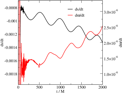
Figure 8: Comparison between $ds/dt$ and $d\omega/dt$ for the same simulation as shown in Fig. 7.

To gauge the importance of this effect, we compare the time derivatives of spatial separation $s$ of the black hole apparent horizons to that of $\omega$. Because $s$ is calculated as an integral using the spatial metric, it is a physical quantity that’s not directly influenced by the control system. We therefore expect $ds/dt$ to settle down much more quickly than $d\omega/dt$. This is indeed the case as shown by Fig. 8. By visual inspection, it is clear that the deviation from a smooth (drifting) sinusoidal curve is pronounced in $d\omega/dt$ up to around $t=1500$M. On the other hand, $ds/dt$ appears to have settled down before $t=500$M. In the next section, we introduce a procedure that helps avoid even those high frequency oscillations at the beginning of $ds/dt$.

IV The joint-elimination algorithm

We now turn to the joint-elimination method outlined in Sec. I, which as already alluded to in that section, ameliorates those longer-lasting impacts of JR examined in Sections III.2 and III.3. This section is devoted to a brief description of the technical details of how we process the periodically intercepted evolution data and feed it through the initial data solver.

For the purpose of this paper, the only adjustments to the intercepted data are those required by eccentricity reduction, and details of our implementation of these adjustments in the stop-and-go operation differs significantly from the traditional approach described in Sec. II.2. First, the changes to the black holes’ radial and tangential velocities are now applied at the time of stopping $t=T_{\text{stop}}$ instead of initial time $t=0$, so the phase $\phi$ in Eq. (24) should be changed to that at $T_{\text{stop}}$. This can be accomplished by substituting $t$ in Eq. (20) with $t-T_{\text{stop}}$. Migrating to $T_{\text{stop}}$ affords us some flexibility. For example, we can now choose $T_{\text{stop}}$ such that $\phi=0,\pi$ or $\phi=\pi/2,3\pi/2$ so that only one of $\delta\Omega_{\text{stop}}$ and $\delta\dot{a}_{\text{stop}}$ is non-vanishing. For the simple example case we look at in Sec. V, there doesn’t appear to be any benefit in doing so, yet this option may become useful in more complicated binary configurations.

Given $(\delta\Omega_{\text{stop}},\delta\dot{a}_{\text{stop}})$ from Eq. (24) with the appropriate $\phi$, we now turn to the problem of implementing them. Because the mean curvature for the intercepted data is no longer vanishing, the dual frame procedure used in Sec. II.1 is no longer applicable, and we solve the XCTS equations directly in the inertial frame instead. In any case we have realistic $\partial_{t}K$ and $\tilde{u}_{ij}$, so there is no need to invoke the co-rotating frame. To implement $(\delta\Omega_{\text{stop}},\delta\dot{a}_{\text{stop}})$, we simply add them to the $\xi_{\rm rad}^{i}$ term that appears in the inertial frame inner boundary condition (22), which now becomes

$$\xi^{i}_{\rm rad}=\left(({\bf\Omega}_{\text{stop}}+\delta{\bf\Omega}_{\text{stop}})\times{\bf r}\right)^{i}+\left(\dot{a}_{\text{stop}}+\delta\dot{a}_{\text{stop}}\right)r^{i}.$$ (37)

Because the elliptic solver is not allowed to change boundary conditions, we do not need to worry that the solution to the XCTS equations simply revert back to the original intercepted data.

The simplest way to impose this new shift inner boundary condition is to weigh $(\delta{\bf\Omega}_{\text{stop}}\times{\bf r})^{i}+\delta\dot{a}_{\text{stop}}r^{i}$ by Gaussian envelops like those in Eq. (14), add the result onto the intercepted shift, and then extract the Dirichlet boundary condition from this augmented shift. This is done at both the inner (excision surfaces) and outer (the outer edge of the computational domain instead of $r\rightarrow\infty$) boundaries. Dirichlet boundary conditions using intercepted lapse is used for $N$, while uniform constant $1$ is used for $\psi$. The augmented shift itself provides a smooth (no discontinuity at the boundaries) initial guess of $N^{i}$ for the elliptic solver, while intercepted $N$ and constant field $\psi=1$ complete the rest of the initial guesses.

In addition to physical data, many auxiliary quantities are needed during an evolution using the SpEC code, such as the parameters used by the feedback control system mentioned in Sec. III.3. Because these parameters don’t change physics, we simply keep their value unchanged through the stop-and-go operation, even though the physical data has been altered slightly. This causes small oscillations in the parameters immediately after relaunch, which does not signal the existence of a new physical junk radiation and tends to settle down relatively quickly for small $(\delta\Omega_{\text{stop}},\delta\dot{a}_{\text{stop}})$ (See Fig. 11 for an example).

Another complication is that although the XCTS equations are solved with a multidomain spectral method Pfeiffer et al. (2003), its current preferred domain decomposition is different from that of the time evolution Szilagyi et al. (2009), due partially to historical reasons. A consequence of involving all these different numerical grids is that filtering on the spectral coefficients Szilagyi et al. (2009) is required to avoid aliasing effects when copying data between them.

V The results

In this section, we demonstrate that the three issues targeted by our joint-elimination procedure, namely junk radiation, orbital eccentricity and constraint violation, are resolved as expected. We do so through illustration using the standard example simulation. For comparison, we also carry out the traditional eccentricity reduction procedure of repeatedly starting the simulation from $t=0$ using initial states constructed with analytical free-data. We will refer to this alternative as the “traditional approach”.

V.1 Junk radiation reduction

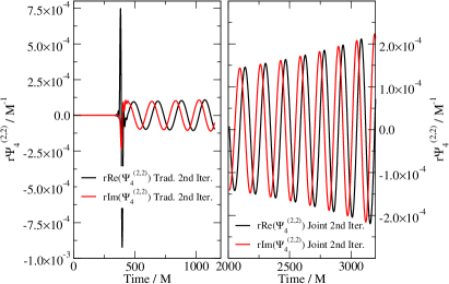
Figure 9: The $(l=2,m=2)$ mode $r\Psi_{4}$ waveforms extracted at coordinate radius of $380$M, from the evolutions using initial data generated with the traditional (left panel) and joint-elimination (right panel) approaches.

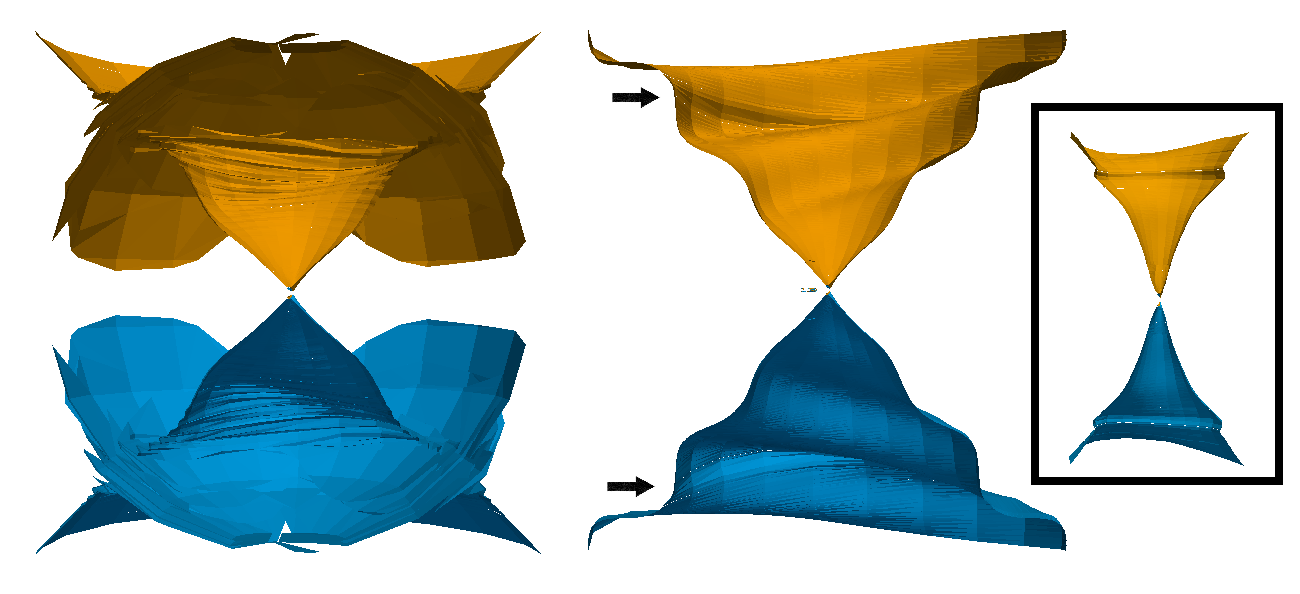
Figure 10: Left: Two contours of $\theta^{t}$ in the simulation starting from the traditional approach initial data, after eccentricity has been removed. There is an obvious junk pulse moving outwards. Right: Two contours of $\theta^{t}$ in the simulation starting from the joint-elimination approach initial data. The only visible new junk radiation is a pulse of small disturbance moving from the outer boundary inwards, as highlighted by the arrows. The inset in the black frame shows a continuation of a clean simulation (after initial JR has exited), but with outer boundary shifted inwards. A new pulse of JR resulting from the mismatch between bulk data and evolution boundary condition can be seen moving inwards.

Although we are assured, by construction, the primary junk radiation should have passed by the time we are done with the eccentricity reduction iterations, we nevertheless need to make sure that no significant amount of new junk radiation is being introduced by the stop-and-go operation discussed in Sec. IV. Fig. 9 compares the $(l=2,m=2)$ mode waveforms in the final iteration of the traditional and joint-elimination approaches. It confirms that there is no visible junk radiation in the joint-elimination approach waveform.

Next, we move on to the $\theta^{t}$ contours, which are more sensitive JR detectors. These contours are shown in Fig. 10, with the result for traditional approach on the left and joint-elimination approach on the right. The only visible new JR is an incoming pulse from the outer boundary (highlighted by black arrows), which is due to the inconsistency between the outer boundary condition imposed by the evolution system and the initial data inside the computational domain. Specifically, we use the constraint preserving boundary condition (Eq. (95) of Buchman and Sarbach (2006)) that sets the incoming gravitational radiation to zero, while in general such radiation does exist at finite radius. During a continuous evolution, the persistent imposition of the boundary condition forces the incoming radiation to vanish at the outer boundary (which is part of the reason why outer boundary has to be placed far away). However, after we change the black hole velocities and copy data between different grids (introducing aliasing noise), this is no longer exactly true when we relaunch the simulation. The impact of this mismatch can be seen more cleanly if instead of carrying out our stop-and-go operation, we simply restart a stopped simulation, but move the outer boundary inwards to where incoming radiation is still present. The $\theta^{t}$ contours in this case are plotted in the inset of Fig. 10, and we see a similar incoming pulse. This subtle effect is invisible in the waveform shown in Fig. 9.

V.2 Orbital eccentricity reduction

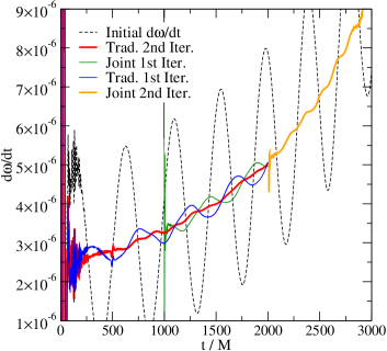
Figure 11: The $d\omega/dt$ curves for the initial and subsequent eccentricity reduction iterations, with both the traditional approach and the joint-elimination approach shown. With both approaches, the oscillations in $d\omega/dt$ become dominated by frequencies higher than the orbital one during the second iteration.

We turn next to the issue of eccentricity reduction. With both the traditional and joint-elimination approaches, we manage to reduce eccentricity from around $0.0033$ to under $0.0001$ within two iterations. With the traditional approach, the sequence of eccentricities is $0.0033\rightarrow 0.00037\rightarrow 0.00009$, and in the joint-elimination approach the sequence is $0.0033\rightarrow 0.00025\rightarrow 0.00005$. Below an eccentricity of $10^{-4}$, the oscillation in $d\omega/dt$ becomes dominated by frequencies higher than orbital frequency (see the red and orange lines in Fig. 11), signaling a possibly non-eccentricity related origin Buonanno et al. (2011), and the fitting formula (20) becomes ill-behaved.

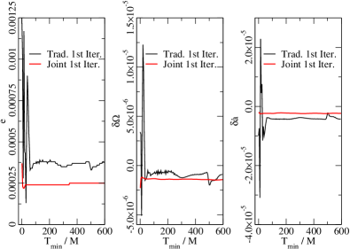
Figure 12: Comparison between the dependence on $T_{\text{min}}$ of $e$ (left panel), $\delta\Omega$ (middle panel) and $\delta\dot{a}$ (right panel) for the traditional and joint-elimination approaches. These parameters are extracted during the first eccentricity reduction iteration. For better visual comparison between curves, the time axis for the joint-elimination approach has been shifted such that it appears to start at $t=0$. The simulations in both approaches are evolved for a sufficiently long time to accommodate $T_{\text{max}}$ for all $T_{\text{min}}$ used in this figure.

Although for this simple example, the final eccentricity value is only marginally smaller in the joint-elimination approach as compared to the traditional approach, the improvement in the stability (against $T_{\text{min}}$) of estimation for $e$, and subsequently $\delta\Omega$ and $\delta\dot{a}$ (we drop the subscripts for brevity), is appreciable in the joint-elimination approach, making the eccentricity reduction process more robust. To demonstrate this stability, we plot $e$, $\delta\Omega$ and $\delta\dot{a}$ against $T_{\text{min}}$ in Fig. 12, obtained during the first iteration in both the traditional and joint-elimination approaches. Aside from the initial disturbance caused by JR directly, the quality of parameter estimation in the traditional approach continues to suffer for a long period afterwards, while the situation is improved with the joint-elimination approach.

V.3 Constraint violation reduction

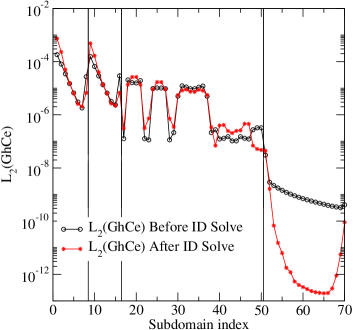
Figure 13: The $L_{2}$ norm of the GhCe constraint measurement within individual subdomains, calculated at the beginning of the first iteration in the joint-elimination approach. For comparison, we also show the constraint violation just before the stop-and-go operation, i.e. before the initial data solver is invoked. The horizontal axis is the index for the subdomains. The sectors separated by vertical lines contain, from left to right, inner spherical shells around one of the black holes extending from the excision boundary to $4.5$M, similar shells around the other black hole, some cylindrical shapes filling up the region in-between and surrounding the inner spherical shells, and finally outer spherical shells extending from $45$M to $480$M that enclose all of the aforementioned subdomains.

Finally, we examine the consequence of re-imposing constraints when we periodically feed the data through the initial data solver, which by construction solves for the constraint parts of the Bianchi identity. Furthermore, when we assemble the output of the initial data solver into variables used by the generalized harmonic evolution system Lindblom et al. (2006a), we also re-impose the secondary constraints coming from reducing a second order partial differential equation into a system of first order equations. For example, one of the evolution variables is $\kappa_{abc}$, which should relate to spacetime metric ${}^{(4)}{\bf g}$ by

$$\kappa_{0ab} = -\frac{1}{N}\left(\partial_{t}{}^{(4)}g_{ab}-N^{i}\partial_{i}{}^{(4)}g_{ab}\right),$$

$$\kappa_{iab} = \partial_{i}{}^{(4)}g_{ab}.$$ (38)

This relationship is reaffirmed when we reconstruct $\kappa$ from the spatial and temporal derivatives of the metric. These attributes of the stop-and-go operation would help clean up the JR-excited constraint violation discussed in Sec. III.2.

In this subsection, we verify that the effectiveness of the initial data solver is not compromised by the complexity of numerical metric data, or our black hole velocity adjustments. In other words, the constraint violation is reduced as expected after an iteration of the stop-and-go operation. To this end, we compare the constraint violation at the beginning ($t=994.5$M) of the first iteration in the joint-elimination approach, to that just before the stop-and-go operation. We plot in Fig. 13 the Generalized Harmonic Constraint Energy (GhCe) for different subdomains in these two cases. The points in the right-most sector are associated with spherical shell subdomains situated on the outside of the entire computational domain. Because the grid structure in these regions are least appropriate for resolving JR, we expect the reduction in constraint violation to be most pronounced for them, and this is exactly what we observe.

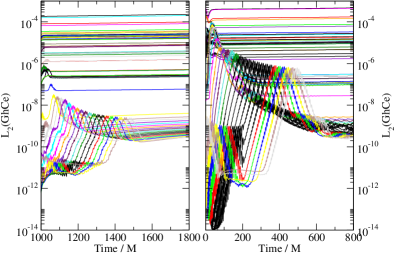
Figure 14: The evolution of $L_{2}(\text{GhCe})$ broken down to individual subdomains, for the joint-elimination (left panel) and traditional (right panel) approaches. In both cases, the constraint violation asymptotes to the levels sustainable by the (shared) resolution of the simulations. During the intermediate time, constraint violation is smaller for the joint-elimination case due to the reduction in JR. The curves near the bottom of the plots correspond to outer spherical shell subdomains.

When we launch the numerical evolution from these initial data, the constraint violation will rise towards the levels sustainable by our low simulation resolution. One may of course increase the resolution and/or adopt a more sophisticated domain decomposition to take better advantage of the clean initial data. However, even for low resolution, the constraint violation behaves much less aggressively during the intermediate time, due to the reduction in JR. This is graphically depicted in Fig. 14, in which we plot the $L_{2}(\text{GhCe})$ growth per subdomain for the joint-elimination and traditional approaches, during the first eccentricity reduction iteration.

VI Conclusion

In this paper we have argued that the constraint violation excited by under-resolved junk radiation would be long-lived, motivating the need to remove JR’s impacts with a method better than simply waiting for it to exit. We also propose that the robustness of the eccentricity reduction procedure could be improved if we do not have to contend with JR. We then introduced a practical method for achieving these goals. In short, we link up the iterations in an eccentricity reduction procedure by feeding the final numerical metric data in the previous iteration into the initial data solver for the next. The effectiveness and advantages of our approach is then demonstrated with a particular binary example.

Aside from generating constraint violation and disturbing control systems, another consequence of JR is that it alters the physical parameters of the black holes. For example the spins of the black holes may drop under the influence of JR, which hampers efforts at creating initial data for high-spin black hole binaries. The joint-elimination approach introduced here can be adapted to address this problem. Namely we could change the $N^{i}_{\parallel}$ term in the inertial frame boundary condition Eq. (22) during each iteration, in order to dial up the black hole spins in stages. Similar arrangements can be made for an adjustment of the black holes’ masses. Applications such as this will be the subject of further studies.