Long-range interactions in randomly driven granular fluids

Abstract

We study the long-range spatial correlations in the nonequilibrium steady state of a randomly driven granular fluid with the emphasis on obtaining the explicit form of the static structure factors. The presence of immobile particles immersed in such a fluidized bed of fine particles leads to the confinement of the fluctuation spectrum of the hydrodynamic fields, which results in effective long-range interactions between the intruders. The analytical predictions are in agreement with the results of discrete element method simulations. By changing the shape and orientation of the intruders, we address how the effective force is affected by small changes in the boundary conditions.

I Introduction

A freely evolving gas of inelastically colliding particles behaves differently from a regular gas due to the dissipative nature of collisions. Starting with a uniformly distributed granular gas, the system first enters a homogeneous cooling state, where the kinetic energy decays as $t^{-2}$, known as Haff’s law Haff83 . However, this regime is unstable against spatial fluctuations of collision frequency, leading to a crossover to a regime where the energy decreases as $t^{-d/2}$ in d dimensions and eventually dense clusters appear Brito98 ; Goldhirsch93 ; Efrati05 ; Cattuto04 . In order to maintain the dynamics, energy must be pumped into the system from an external driving source e.g. by shaking, vibrating, or shearing. As a result, the energy input competes against the energy dissipation due to inelastic collisions, and the system is driven into a steady state. Since the energy insertion is spatially inhomogeneous in the above mentioned boundary heating methods, a uniformly heating approach had been proposed as a paradigm allowing to study a homogeneous stationary state Williams96 ; Peng98 ; vanNoije99 ; The system is supposed to be in contact with a thermal bath which supplies energy by means of instantaneous random forces acting on all particles. The resulting dynamics, in two dimensions, is reminiscent of the motion of thin disks on an air table in quasi-2D experiments Oger96 . The uniformly driven granular fluid reaches a nonequilibrium steady state due to the random nature of energy gain and loss, and exhibits long-range hydrodynamic correlations. These spatial correlations decay with distance as $r^{-1}$ and $\ln(1/r)$ in three and two dimensions, respectively vanNoije99 . Similar long-range spatial correlations emerge in freely cooling vanNoije97 or sheared Otsuki09 systems of slightly inelastic granular fluids, even though the anisotropic couplings between the number density and momentum density fluctuations influences the behavior in the sheared case, leading to a different power-law asymptotic form at large $r$ Otsuki09 .

In a thermally fluctuating medium with long-range spatial correlations, one expects that the presence of big intruder particles modifies the boundary conditions and, hence, leads to the modification of the hydrodynamic fluctuations spectrum. As a result, effective interactions between intruders appear which are long-range, in spite of the short-range nature of hard-core interparticle forces. Such interactions are often considered as classical variants of the Casimir force Casimir48 ; Kardar99 . Recent experiments Aumaitre01 ; Zuriguel06 ; Villanueva10 ; GarciaTrujillo13 ; Rivas11 and numerical simulations Sanders05 ; Denisov11 ; Rivas11 ; Cattuto06 ; Shaebani12 confirm that the confinement of fluctuations in fluidized granular media produces spatial hydrodynamic inhomogeneities that are practically strong enough to induce substantial effective interactions between the intruders. Depending on the choice of parameter values, these forces can be either attractive or repulsive and may lead to a variety of collective behaviors Aumaitre01 ; Rivas11 ; GarciaTrujillo13 . Even a single asymmetric object may experience a self-force in a nonequilibrium state Buenzli09 . The interactions emerging in equilibrium state had also been studied by considering two bodies immersed in a solution of macromolecules Asakura54 . Note that we deal with the regime where the interparticle forces are mainly binary collisions. Investigation of the underlying mechanisms when durable frictional contacts dominate the behavior is beyond the scope of the present study.

In this paper we first recall how the fluctuations of the hydrodynamic fields are spatially correlated in a randomly driven granular fluid. We derive the explicit form of the static structure factors, which reflect the spatial correlations of the medium. These quantities are then used to calculate the effective long-range interaction between two immobile big particles immersed in the medium. The method had been used in Ref.Shaebani12 to study the sign change and nonadditivity of the effective force, and to obtain the phase diagram of the transition between repulsive and attractive forces. Here, the main goal is to provide a detailed methodology for obtaining the structure factors and the fluctuation-induced force, as a recipe for further applications and extensions. We also investigate the effect of small changes in the boundary conditions on the effective force, by considering elongated intruders and changing their shape or orientation. The elongated particles are frequent and play important role in nature and industry. The interesting question arises whether fluctuation-induced forces may lead to orientational ordering and alignment of such particles. We investigate this question in a simple case of two elliptical intruders (with fixed centers) by varying their eccentricity and orientations to find the configuration where the intruders experience the maximum possible force.

The paper is organized as follows: In Sec. II we review the theory of randomly driven granular fluids and derive the structure factors, which are used in Sec. III to calculate the effective force between the intruders with circular shapes. This part is the full exposition and expansion of the mode coupling calculations presented in Shaebani12 . The validity of the analytical method is established by means of discrete element method simulations in Sec. IV. Section V is devoted to the investigation of the influence of intruder shape on the effective force, by considering elliptical particles. Finally, Sec. VI contains the discussion of the results and concluding remarks.

II Theory of a randomly driven granular system

In this section, we review the nonequilibrium steady state properties of a randomly driven granular system, and present the explicit form of the structure factors. A detailed description of the theory can be found, e.g., in Refs. vanNoije99 ; vanNoije97 ; Gradenigo11 . Consider a system of $N$ hard spheres (or disks in two dimensions) of mass $m$ and radius $R$ with a Langevin-type equation of motion:

$$m\frac{d^{2}{\bm{r}}_{\text{i}}(t)}{dt^{2}}={\bm{F}}_{\text{i}}(t)+{\bm{\xi}}_{\text{i}}(t),$$ (1)

where ${\bm{F}}_{\text{i}}$ is the total force acting on particle $i$ due to binary inelastic collisions, and ${\bm{\xi}}_{\text{i}}$ is a random force arising from the coupling to an external heat bath. We assume that the random force is drawn from a distribution with zero mean, and with Cartesian components $\alpha$ and $\beta$ satisfying

$$\langle\xi_{\text{i}\alpha}(t)\xi_{\text{j}\beta}(t^{\prime})\rangle=2\Gamma\delta_{\alpha\beta}\delta_{\text{ij}}\delta(t{-}t^{\prime}).$$ (2)

Here, $\langle\cdot\cdot\cdot\rangle$ denotes averaging over the uncorrelated noise source, and $\Gamma$ reflects the noise strength. For the mean rate of energy gain of a single particle in $D$ dimensions one finds the following expression

$$\bigg{\langle}\frac{\partial\mathcal{E}}{\partial t}\bigg{\rangle}_{\!\!\text{gain}}=D\,\Gamma/m.$$ (3)

On the other hand, the mean-field rate of energy loss of a single particle by means of inelastic collisions is given by Enskog ; vanNoije97

$$\bigg{\langle}\frac{\partial\mathcal{E}}{\partial t}\bigg{\rangle}_{\!\!\text{loss}}=-\gamma\>(1{-}\alpha^{2})\>\mathit{f}(n)\>T^{3/2},$$ (4)

where $\gamma$ is a constant (which depends on $D$, $m$, and $R$), $\alpha$ is the normal restitution coefficient, and $\mathit{f}$ is a function of the number density $n$, given in two dimensions by Verlet82

$$\mathit{f}(n){=}n\big{(}1{-}7\phi/16\big{)}\big{/}\big{(}1{-}\phi\big{)}^{2},$$ (5)

with $\phi$ being the volume fraction. It can be seen from Eqs. (3) and (4) that the rate of temperature change is given by $\partial T/\partial t{=}D\Gamma/m{-}\gamma(1{-}\alpha^{2})\mathit{f}(n)T^{3/2}$, thus, the time dependence of temperature can be obtained by the following integration

$$\int_{T_{{}_{0}}}^{T}\displaystyle\frac{dT}{1{-}\displaystyle\frac{m\gamma}{D\Gamma}\big{(}1{-}\alpha^{2}\big{)}\mathit{f}(n)T^{3/2}}=\displaystyle\int_{{{}_{0}}}^{t}\displaystyle\frac{D\Gamma}{m}dt.$$ (6)

We introduce the scaled temperature $\widetilde{T}{\equiv}T/T_{{}_{\text{MF}}}$ (with $T_{{}_{\text{MF}}}{=}[D\Gamma/m\gamma(1{-}\alpha^{2})\mathit{f}(n)]^{2/3}$ being the mean-field steady state temperature), and integrate Eq. (6) to arrive at the following implicit expression for the time evolution of the temperature

$$\ln\Big{(}{\displaystyle\frac{1{+}\displaystyle\sqrt{\widetilde{T}}{+}\widetilde{T}}{1{-}2\displaystyle\sqrt{\widetilde{T}}{+}\widetilde{T}}}\Big{)}-2{\sqrt{3}}\arctan\Big{(}{\displaystyle\frac{2\displaystyle\sqrt{\widetilde{T}}{+}1}{\sqrt{3}}}\Big{)}=\frac{3D\Gamma}{mT_{{}_{\text{MF}}}}\,t-A,$$ (7)

where $A$ is a constant which depends on the initial temperature. The system eventually reaches a nonequilibrium steady state, where the hydrodynamic fields $(T(\bm{r},t),n(\bm{r},t),\bm{v}(\bm{r},t))$ fluctuate around their stationary values $(T_{\text{s}},n_{\text{s}}({=}N/V),0)$, due to the stochastic nature of energy gain and loss ($V$ is the volume of the $D$-dimensional system). It has been proven vanNoije99 that the fluctuations in two dimensions are logarithmically divergent in the system size $L$, which results in a steady temperature higher than $T_{{}_{\text{MF}}}$ ($T_{\text{s}}{-}T_{{}_{\text{MF}}}{\sim}\text{Ln}\>L$). The goal of the next subsection is to investigate the spatial fluctuations of the hydrodynamic fields, and their long-range correlations.

II.1 Hydrodynamic fluctuations

Assuming continuous (coarse-grained) hydrodynamic fields for a weakly inelastic fluid of hard particles, one can describe the system via standard hydrodynamic equations vanNoije99 ; vanNoije00

$$\frac{\partial n(\bm{r},t)}{\partial t} =-{\bm{\nabla}}{\cdot}(n(t){\bm{v}}(t)),$$ (8)

$$\frac{\partial{\bm{v}}(\bm{r},t)}{\partial t} =-{\bm{v}}{\cdot}{\bm{\nabla v}}-\frac{1}{\rho}{{\bm{\nabla}}{\cdot}{\bm{\Pi}}},$$

$$\frac{\partial T(\bm{r},t)}{\partial t} =-{\bm{v}}{\cdot}{\bm{\nabla}}T-\frac{2}{Dn}({\bm{\nabla}}{\cdot}{\bm{J}}+{\bm{\Pi}}{:}{\bm{\nabla}}{\bm{v}})$$

$$\hskip 49.79231pt{+}\bigg{\langle}\frac{\partial\mathcal{E}}{\partial t}\bigg{\rangle}_{\!\!\text{gain}}{-}\bigg{\langle}\frac{\partial\mathcal{E}}{\partial t}\bigg{\rangle}_{\!\!\text{loss}},$$

where $\rho$, $\bm{\Pi}$, and $\bm{J}$ refer to the density, the pressure tensor, and the heat flux, respectively. The last equation is generalized by adding source and sink terms to account for the energy gain from the heat bath and the energy loss due to inelastic collisions. One can linearize Eqs. (8) around the steady state homogeneous values $(T_{\text{s}},n_{\text{s}},0)$ to get the following equations vanNoije99

$$\frac{\partial}{\partial t}\delta n(\bm{r},t) {=}-n{\bm{\nabla}}{\cdot}{\bm{v}},$$ (9)

$$\frac{\partial}{\partial t}\delta\bm{v}(\bm{r},t) {=}-\frac{1}{\rho}\bm{\nabla}p{+}\eta\nabla^{2}\bm{v}{+}(\eta{-}\eta_{{}_{\ell}}){\bm{\nabla\nabla}}{\cdot}{\bm{v}}{+}{\bm{\zeta}}_{1}(\bm{r},t),$$

$$\frac{\partial}{\partial t}\delta T(\bm{r},t) {=}\frac{2c}{Dn}\nabla^{2}\delta T{-}\frac{2p}{Dn}{\bm{\nabla}}{\cdot}{\bm{v}}{-}\delta\bigg{\langle}\frac{\partial\mathcal{E}}{\partial t}\bigg{\rangle}_{\!\!\text{loss}}{+}{\zeta}_{2}(\bm{r},t),$$

with $p$, $c$, $\eta$, and $\eta_{{}_{\ell}}$ being the pressure, the heat conductivity, and the kinetic and longitudinal viscosities, respectively. Since the theory is valid for small inelasticities, $c$, $\eta$, and $\eta_{{}_{\ell}}$ can be approximated by the corresponding values in an elastic hard particle system, obtained from the Enskog theory Enskog . The noise terms ${\bm{\zeta}}_{1}(\bm{r},t)$ and ${\bm{\zeta}}_{2}(\bm{r},t)$ arise from (i) the external noise originating from the random force $\bm{\xi}(t)$ in Eq. (1) vanNoije99 , and (ii) the internal fluctuations around thermal equilibrium, obtained from the fluctuation-dissipation theorem Landau59 ; vanNoije97 .

Next, using Fourier transforms, one replaces the hydrodynamic fluctuating fields $\delta F(\bm{r},t)$ (including $n$, $T$, longitudinal velocity $v_{\!{}_{\ell}}$, and transverse velocity $v_{t}$) with $\delta F(\bm{r},t){=}\int\delta F(\bm{k},t)e^{i\bm{k\cdot r}}d\bm{k}$ to get

$$\left(\begin{array}[]{c}\!\!\frac{\partial}{\partial t}\delta n(\bm{k},t)\\ \\ \!\!\frac{\partial}{\partial t}\delta T(\bm{k},t)\\ \\ \!\!\frac{\partial}{\partial t}\delta v_{\!{}_{\ell}}(\bm{k},t)\\ \\ \!\!\frac{\partial}{\partial t}\delta v_{t}(\bm{k},t)\end{array}\!\!\right){=}-{\bm{M}(k)}\!\!\left(\begin{array}[]{c}\!\!\delta n(\bm{k},t)\\ \!\!\delta T(\bm{k},t)\\ \!\!\delta v_{\!{}_{\ell}}(\bm{k},t)\\ \!\!\delta v_{t}(\bm{k},t)\end{array}\!\!\right){+}\left(\begin{array}[]{c}\!\!\zeta_{{}_{n}}(\bm{k},t)\\ \!\!\zeta_{{}_{T}}(\bm{k},t)\\ \!\!\zeta_{v}{{}_{\!{}_{\ell}}}(\bm{k},t)\\ \!\!\zeta_{v}{{}_{\!{}_{t}}}(\bm{k},t)\end{array}\!\!\right),$$ (10)

with

$${\bm{M}(k)}{=}\!\!\left(\begin{array}[]{cccc}\!\!\!\!0&0&\!ikn&\!\!\!0\\ \\ \!\!\!\!\displaystyle\frac{(1{-}\alpha^{2})\omega T}{D\;\mathit{f}(n)}\frac{d\mathit{f}(n)}{dn}&\displaystyle\frac{2ck^{2}}{D\,n}{+}\frac{3\omega(1{-}\alpha)^{2}}{2\,D}&\!\displaystyle\frac{2ikp}{D\,n}&\!\!\!0\\ \\ \!\!\!\!\displaystyle\frac{ik}{n}\left(\displaystyle\frac{\partial p}{\partial\rho}\right)_{\!T}&\displaystyle\frac{ikp}{\rho T}&\!\eta_{{}_{\ell}}k^{2}&\!\!\!0\\ \\ \!\!\!\!0&0&\!0&\!\!\!\eta k^{2}\end{array}\!\!\!\!\right)\!\!.$$ (11)

Here, $\omega{\sim}\mathit{f}(n)\sqrt{T}$ is the collision frequency obtained from the Enskog theory. The component $\zeta_{{}_{n}}(\bm{k},t)$ of the white noise vector $\bm{\zeta}(\bm{k},t)$ in Eq. (10) is indeed zero, and the rest of the components (i.e. $\zeta_{{}_{T}}(\bm{k},t)$, $\zeta_{v}{{}_{\!{}_{\ell}}}(\bm{k},t)$, and $\zeta_{v}{{}_{\!{}_{t}}}(\bm{k},t)$) are Gaussian with correlations

$$\langle\zeta_{\text{i}}(\bm{k},t)\zeta_{\text{j}}(-\bm{k},t^{\prime})\rangle=VC_{{}_{\text{ij}}}(k)\delta(t{-}t^{\prime}).$$ (12)

By taking Fourier transforms of ${\bm{\zeta}}_{1}(\bm{r},t)$ and ${\bm{\zeta}}_{2}(\bm{r},t)$, the nonzero elements of the matrix ${\bm{C}}(k)$ are determined as follows vanNoije99

$$\begin{aligned} C_{{}_{\text{22}}}(k)&{=}\displaystyle\frac{8T\Gamma}{D\rho}{+}\displaystyle\frac{8cT^{2}}{D^{2}n^{2}}k^{2},\\ \\ C_{{}_{\text{33}}}(k)&{=}\displaystyle\frac{2n\Gamma}{\rho^{2}}{+}\displaystyle\frac{2\eta_{{}_{\ell}}T}{\rho}k^{2},\\ \\ C_{{}_{\text{44}}}(k)&{=}\displaystyle\frac{2n\Gamma}{\rho^{2}}{+}\displaystyle\frac{2\eta T}{\rho}k^{2}.\end{aligned}$$ (13)

Once the hydrodynamic fluctuations are determined, one can calculate the structure factors $S_{{}_{ab}}(k)$, which are indeed the Fourier transforms of the spatial correlation functions. The structure factors in the nonequilibrium steady state are given by

$$S_{{}_{ab}}(k){=}\lim_{t\to\infty}\frac{1}{V}\langle\delta a(\bm{k},t)\,\delta b(-\bm{k},t)\rangle.$$ (14)

Let us denote $\bm{S}(k)$ as a $4\times 4$ matrix with elements labeled by $n$, $T$, $v_{\!{}_{\ell}}$, and $v_{t}$:

$$\bm{S}(k){=}\!\left(\begin{array}[]{cccc}\!\!S_{nn}(k)&S_{nT}(k)&S_{nv_{\!{}_{\ell}}}(k)&S_{nv_{\!{}_{t}}}(k)\\ \\ \!\!S_{T\!n}(k)&S_{TT}(k)&S_{Tv_{\!{}_{\ell}}}(k)&S_{T\!v_{\!{}_{t}}}(k)\\ \\ \!\!S_{v_{\!{}_{\ell}}\!n}(k)&S_{v_{\!{}_{\ell}}\!T}(k)&S_{v_{\!{}_{\ell}\!}v_{\!{}_{\ell}}}(k)&S_{v_{\!{}_{\ell}}\!v_{\!{}_{t}}}(k)\\ \\ \!\!S_{v_{\!{}_{t}}\!n}(k)&S_{v_{\!{}_{t}}\!T}(k)&S_{v_{\!{}_{t}}\!v_{\!{}_{\ell}}}(k)&S_{v_{\!{}_{t}}\!v_{\!{}_{t}}}(k)\end{array}\!\!\right)\!.$$ (15)

By integrating Eqs. (10) and using Eq. (12) one arrives at the following equation for the time evolution of $\bm{S}(k)$

$$\frac{\partial}{\partial t}{\bm{S}(k)}=-{\bm{M}(k)}{\bm{S}(k)}-{\bm{S}(k)}{\bm{M}^{T}(-k)}+\bm{C}(k),$$ (16)

where $\bm{M}^{T}$ is the transpose of $\bm{M}$. Setting the left-hand side to zero, the steady state values of the structure factors can be calculated. Among the elements of $\bm{S}(k)$, we are interested in $S_{nn}(k)$ and $S_{nT}(k)$ obtained as

$$S_{nn}(k)=\frac{M_{{}_{13}}\big{(}M_{{}_{22}}M_{{}_{32}}^{2}C_{{}_{22}}+M_{{}_{32}}^{2}M_{{}_{33}}C_{{}_{22}}-M_{{}_{22}}^{3}C_{{}_{33}}+M_{{}_{13}}M_{{}_{22}}M_{{}_{31}}C_{{}_{33}}-M_{{}_{13}}M_{{}_{21}}M_{{}_{32}}C_{{}_{33}}-M_{{}_{22}}^{2}M_{{}_{33}}C_{{}_{33}}\big{)}}{2\big{(}M_{{}_{22}}M_{{}_{31}}-M_{{}_{21}}M_{{}_{32}}\big{)}\bigg{(}\big{(}M_{{}_{22}}+M_{{}_{33}}\big{)}\big{(}M_{{}_{23}}M_{{}_{32}}-M_{{}_{22}}M_{{}_{33}}\big{)}+M_{{}_{13}}\big{(}M_{{}_{21}}M_{{}_{32}}+M_{{}_{31}}M_{{}_{33}}\big{)}\bigg{)}},$$ (17)

and

$$S_{nT}(k)=\frac{M_{{}_{13}}\bigg{(}M_{{}_{31}}\big{(}-M_{{}_{32}}M_{{}_{33}}C_{{}_{22}}+M_{{}_{22}}M_{{}_{23}}C_{{}_{33}}\big{)}+M_{{}_{21}}\big{(}-M_{{}_{32}}^{2}C_{{}_{22}}-M_{{}_{23}}M_{{}_{32}}C_{{}_{33}}+M_{{}_{22}}\big{(}M_{{}_{22}}+M_{{}_{33}}\big{)}C_{{}_{33}}\big{)}\bigg{)}}{2\big{(}M_{{}_{22}}M_{{}_{31}}-M_{{}_{21}}M_{{}_{32}}\big{)}\bigg{(}\big{(}M_{{}_{22}}+M_{{}_{33}}\big{)}\big{(}M_{{}_{23}}M_{{}_{32}}-M_{{}_{22}}M_{{}_{33}}\big{)}+M_{{}_{13}}\big{(}M_{{}_{21}}M_{{}_{32}}+M_{{}_{31}}M_{{}_{33}}\big{)}\bigg{)}}.$$ (18)

Because of the dominant contribution of small wave numbers $k$, one can approximate $S_{nn}(k)$ and $S_{nT}(k)$ by their leading terms ($\mathcal{O}(1/k^{2})$) which leads to

$$S_{nn}(k)\simeq\frac{-27\omega^{2}T^{2}n^{3}\rho(1{-}\alpha^{2})^{2}}{4D\bigg{[}\bigg{(}\displaystyle\frac{2np}{\mathit{f}(n)}\displaystyle\frac{d\mathit{f}(n)}{dn}-3\rho(\displaystyle\frac{\partial p}{\partial\rho})_{\!{}_{T}}\bigg{)}\bigg{(}6p^{2}+\displaystyle\frac{2Dn^{2}pT}{\mathit{f}(n)}\displaystyle\frac{d\mathit{f}(n)}{dn}+\displaystyle\frac{9(1{-}\alpha^{2})n\eta_{{}_{\ell}}\omega\rho T}{2}\bigg{)}\bigg{]}}\displaystyle\frac{1}{k^{2}},$$ (19)

and

$$S_{nT}(k)\simeq\frac{9\omega^{2}T^{3}n^{3}\rho(1{-}\alpha^{2})^{2}\displaystyle\frac{d\mathit{f}(n)}{dn}}{2D\mathit{f}(n)\bigg{[}\bigg{(}\displaystyle\frac{2np}{\mathit{f}(n)}\displaystyle\frac{d\mathit{f}(n)}{dn}-3\rho(\displaystyle\frac{\partial p}{\partial\rho})_{\!{}_{T}}\bigg{)}\bigg{(}6p^{2}+\displaystyle\frac{2Dn^{2}pT}{\mathit{f}(n)}\displaystyle\frac{d\mathit{f}(n)}{dn}+\displaystyle\frac{9(1{-}\alpha^{2})n\eta_{{}_{\ell}}\omega\rho T}{2}\bigg{)}\bigg{]}}\displaystyle\frac{1}{k^{2}}.$$ (20)

Note that the validity of the mode coupling theory presented in this section is restricted to the long wavelength range, where $k_{\text{max}}{<}\text{min}[2\pi/l^{*},\pi/R]$ (with $l^{*}$ being the mean free path and $R$ the particle radius). The wave numbers are limited also by the system size, so that $2\pi/L{\leq}k_{\text{min}}$. It is also notable that the approximate value of $S_{nn}(k)$ [Eq. (19)] is indeed independent of the noise strength, while $S_{nT}(k)$ [Eq. (20)] is proportional to $\Gamma^{2/3}$.

III Long range interactions between intruder particles

The fluctuating hydrodynamic fields in the nonequilibrium steady state of a uniformly driven medium are spatially homogeneous, as discussed in Sec. II. However, in the presence of large immobile particles immersed in the granular fluid, the fluctuation spectrum would be modified according to the new boundary conditions, resulting in inhomogeneous fields. In the following, we analyse the pressure fluctuations $\delta p(\bm{r},t)$ (in two dimensions for simplicity) and show how geometric constraints lead to average pressure difference around the intruder particles. Let us start with the Verlet-Levesque equation of state for a hard disk system Verlet82

$$p(n,T)=g(n)T,$$ (21)

with $g(n){=}n(1+\phi^{2}/8)/(1-\phi)^{2}$, where $\phi{=}\pi R^{2}n$ is the volume fraction. We expand $p(n,T)$ up to second order around the steady state values $(n_{\text{s}},T_{\text{s}})$

$$\delta p(\bm{r},t){=}p(\bm{r},t){-}p(n_{\text{s}},T_{\text{s}})\simeq\frac{1}{2}T_{\text{s}}\frac{d^{2}g}{dn^{2}}\big{|}_{{}_{n{=}n_{\text{s}}}}\big{(}\delta n(\bm{r},t)\big{)}^{2}+$$ (22)

$$g(n_{\text{s}})\delta T(\bm{r},t){+}T_{\text{s}}\frac{dg}{dn}\big{|}_{{}_{n{=}n_{\text{s}}}}\delta n(\bm{r},t){+}\frac{dg}{dn}\big{|}_{{}_{n{=}n_{\text{s}}}}\delta n(\bm{r},t)\delta T(\bm{r},t).$$

The statistical average of $\delta p(\bm{r},t)$ over the random noise source is then given by

$$\langle\delta p(\bm{r},t)\rangle{=}$$ (23)

$$\frac{dg}{dn}\big{|}_{{}_{n{=}n_{\text{s}}}}\langle\delta n(\bm{r},t)\delta T(\bm{r},t)\rangle{+}\frac{1}{2}T_{\text{s}}\frac{d^{2}g}{dn^{2}}\big{|}_{{}_{n{=}n_{\text{s}}}}\langle\big{(}\delta n(\bm{r},t)\big{)}^{2}\rangle,$$

and finally, by employing the Fourier transforms of the fluctuations, one obtains the local pressure fluctuations as a function of the static structure factors

$$\delta p(k){\sim}\int\bigg{(}\frac{dg}{dn}\big{|}_{{}_{n{=}n_{\text{s}}}}S_{nT}(k){+}\frac{1}{2}T_{\text{s}}\frac{d^{2}g}{dn^{2}}\big{|}_{{}_{n{=}n_{\text{s}}}}S_{nn}(k)\bigg{)}dk.$$ (24)

The upper bound of integration is $k_{\text{max}}{=}2\pi/\text{max}[l^{*},2R]$ (as discussed in the previous section) to ensure that the hydrodynamic description is valid. The lower bound of the allowed wave numbers is restricted by the geometric constraints. Hence, the presence of intruder particles would change the local pressure fluctuations, leading to a net pressure difference around each intruder. As a result, the immersed particles receive forces which can be interpreted as effective long-range interactions between them.

As an illustrating example, we consider a system with two fixed intruders A and B with the same radius $R_{{}_{I}}$ (see Fig. 1) and compare the pressure fluctuations at two points 1 and 2 which have the same $y$ coordinates and located on opposite sides of particle B. While the spectrum along $y$ direction at both points is restricted to the same limits, the allowed wave vectors in $x$ direction are confined to the horizontal distances $D_{{}_{\text{in}}}$ and $D_{{}_{\text{out}}}$ given by

$$\begin{aligned} D\!_{{}_{\text{in}}}\!(y)&{=}D\!_{{}_{\text{AB}}}\!\!-\!2\displaystyle\sqrt{R_{{}_{I}}^{2}\!\!-\!\!y^{2}},\\ D\!_{{}_{\text{out}}}\!(y)&{=}L\!-\!D\!_{{}_{\text{AB}}}\!\!\!-\!\!2\displaystyle\sqrt{R_{{}_{I}}^{2}\!\!-\!\!y^{2}}.\end{aligned}$$ (25)

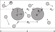
Figure 1: Sketch of the two dimensional system.

Therefore, the local fluctuation of pressure is different at these two points, which gives rise to an average pressure difference

$$\Delta p(y){=}\bigg{(}\int_{2\pi\!/\!D\!_{{}_{\text{in}}}\!\!(y)}^{k_{{}_{\text{max}}}}\!\!\!\!\!\!\!\!\!dk_{{}_{x}}\!\!-\!\!\int_{2\pi\!/\!D\!_{{}_{\text{out}}}\!(y)}^{k_{{}_{\text{max}}}}\!\!\!\!\!\!\!\!\!dk_{{}_{x}}\bigg{)}\!\!\int_{k_{{}_{\text{min}}}\!\!(y)}^{k_{{}_{\text{max}}}}\!\!\!\!\!\!\!dk_{{}_{y}}\>g(k_{{}_{x}},k_{{}_{y}}),$$ (26)

where $g(k_{{}_{x}},k_{{}_{y}})$ is the integrand in Eq. (24). The total effective force $F$ acting on particle B can be obtained by integrating the pressure difference over the surface of the particle

$$F=\int_{-R_{{}_{I}}}^{R_{{}_{I}}}\Delta p(y)dy.$$ (27)

The magnitude and sign of the resulting force depends on $\Delta p(y)$. In general, one should solve $\Delta p{=}0$ to get the crossover point between attractive and repulsive forces. However, using the approximate values of the structure factors $S_{\text{nn}}(k)$ and $S_{\text{nT}}(k)$ [Eqs. (19) and (20)], i.e. only the leading terms ($\mathcal{O}(1/k^{2})$), the integrand in Eq. (26) can be written as $g(k){\sim}\frac{f(n,\alpha)}{k^{2}}$. Therefore, the function $f(n,\alpha)$ can be taken out from the integral, and the transition point is approximately obtained by setting $f(n,\alpha)$ to zero, which leads e.g. to $\phi_{c}{\sim}0.57$ for $\alpha{=}0.8$. The transition point in general is determined by the restitution coefficient, the density, and the distance between the intruders Shaebani12 , thus, one should use the full expressions of the structure factors [Eqs. (17) and (18)]. In the next section, we compare the mode coupling predictions with the results obtained from the simulations.

IV Simulation details

IV.1 The model

We consider a two-dimensional granular gas by means of discrete element method simulations. The system consists of $N{=}3000$ identical rigid disks of radius $R$ and mass $m$ interacting via inelastic collisions with the normal coefficient of restitution $\alpha{=}0.8$ for all collisions. In order to provide a spatially homogeneous state and exclude the undesired effects of side walls, periodic boundary conditions are applied in both directions of the square-shaped system of length $L{=}200R$. Two immobile rigid intruder particles of radius $R_{{}_{I}}{=}10R$ and infinite mass and moment of inertia are immersed in the granular gas bed, separated by a distance $D_{\!{}_{\text{AB}}}{=}30R$ (see Fig. 1). The interaction with the heat bath is modeled in a similar way as in Refs. Peng98 ; vanNoije99 ; Cattuto06 ; Shaebani12 , where the momentum of each particle is perturbed instantaneously at each time step $\Delta t$ by a random amount taken from a Gaussian distribution with zero mean and a given variance $\sigma$. We note that the assumption of the Gaussian white noise is satisfied in the limit $\sigma{\to}0$, and providing that the mean free time $\tau^{*}$ of the granular gas remains much larger than $\Delta t$. Another point is that the total linear momentum of the system is not necessarily conserved in our simulations, since we do not set the sum of noise vectors to zero at each time step. However, the deviation decreases as $1/N$ and vanishes in the limit of large $N$.

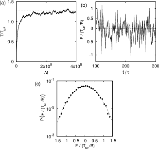
Figure 2: (a) Time evolution of temperature $T$ (scaled by $T_{{}_{\text{MF}}}$) starting from a random initial state. The dashed line indicates the final stationary level. (b) A typical sequence of the fluctuation-induced forces $F$ scaled by $T_{{}_{\text{MF}}}/R$. (c) The probability distribution of $F$ collected over $10^{8}$ time steps. The dashed line shows the best fit with a Gaussian distribution centered on $0.015T_{{}_{\text{MF}}}/R$.

IV.2 Results

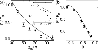
Figure 3: The effective force $F$ scales by $F_{{}_{0}}$ in terms of (a) the distance $D\!_{{}_{\text{AB}}}$ between the intruders, and (b) the volume fraction $\phi$. The solid lines correspond to the mode coupling results discussed in Sec. III. Inset: Same plot as in (a) but on a log-log scale. The dashed line ${\sim}D_{\!{}_{\text{AB}}}^{-2}$ is a guide to the eye.

Starting from a random initial state, the driven gas finally converges to a nonequilibrium steady state, as shown in Fig. 2(a). Then after the system relaxes, we investigate the effective interaction between the two fixed intruders. The total force exerted by the small beads on each intruder during the time interval $\tau$ ($\tau\!\!\sim\!\!250$ collisions per particle) is measured. Figure 2(b) displays the fluctuating nature of the resulting consecutive forces, therefore, this quantity is averaged over more than $10^{4}$ time intervals $\tau$ to suppress the observed large fluctuations. The probability distribution of the data measured along the $x$ axis, shown in Fig. 2(c), can be well fitted by a Gaussian Bartolo02 with the average value $0.015T\!_{{}_{\text{MF}}}/R\!\equiv\!F_{{}_{0}}$ and the standard deviation $\sigma{=}0.612T\!_{{}_{\text{MF}}}/R$. The fluctuations are about two orders of magnitude larger than the average value, indicating that very long simulations are required to measure the forces with relatively small numerical errors. Repeating a similar procedure along the $y$ axis leads to almost zero force within the accuracy of our measurements. $F_{{}_{0}}$ can be considered as the magnitude of the effective long-range force acting between intruders A and B, which is repulsive in this case.

Next we compare the simulation results with the mode coupling predictions obtained from Eqs. (24)-(27) using the full expressions of the structure factors [Eqs. (17) and (18)]. In Fig. 3(a), the force is shown as a function of the distance between the intruders. The interaction is weakened with increasing the distance, and vanishes at $D\!_{{}_{\text{AB}}}{=}L/2$ as expected from the symmetry. By varying the density of the small grains, it is shown in Fig. 3(b) that the sign of the force changes as the volume fraction exceeds a threshold value $\phi_{{}_{c}}\sim 0.57$. The analytical results are also shown in Fig. 3 (solid lines). The agreement is satisfactory, however, the mode coupling method slightly overestimates the force. The deviation can be attributed to the fact that the fluctuations on the opposite sides of the intruder are indeed correlated, which is not taken into account in the mode coupling calculations Cattuto06 ; Shaebani12 . We also point out that using the approximate values of the structure factors with leading terms of order $1/k^{2}$ [Eqs. (19) and (20)] would lead to qualitatively similar results but with more than $10\%$ errors compared with the full expressions [Eqs. (17) and (18)]. A more detailed study of the transition behavior, and further comparison between theoretical and simulation results can be found in Shaebani12 .

V Influence of shape

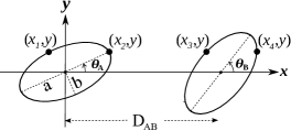
Figure 4: Schematic picture depicting the two elliptical intruders and their orientations.

As demonstrated in the previous sections, the fluctuation-induced force originates from the confinement of the fluctuation spectrum due to geometric constraints imposed by intruders. Two questions arise: How sensitive is the force to the tiny changes in the boundary conditions induced by changing the shape of the intruders? and is the fluctuation-induced interaction able to align elongated particles or create patterns of orientational order? In this section we modify the intruders shape and use the mode coupling method to analytically calculate the corresponding effective forces between two elongated intruders. Numerical simulations to study this effect would be extremely time consuming and are beyond the scope of the present investigation. Instead of circular intruders, here we choose elliptical particles with radii $a$ and $b$ ($b{<}a$), as shown in Fig. 4. By defining

$$\begin{aligned} c_{{}_{1}}&{=}(b^{2}\text{cos}^{2}\theta_{\!{}_{A}}{+}a^{2}\text{sin}^{2}\theta_{\!{}_{A}})/a^{2}b^{2},\\ c_{{}_{2}}&{=}(b^{2}\text{sin}^{2}\theta_{\!{}_{A}}{+}a^{2}\text{cos}^{2}\theta_{\!{}_{A}})/a^{2}b^{2},\\ c_{{}_{3}}&{=}(b^{2}{-}a^{2})\text{sin}\theta_{\!{}_{A}}\text{cos}\theta_{\!{}_{A}}/a^{2}b^{2},\\ c_{{}_{4}}&{=}(b^{2}\text{cos}^{2}\theta_{\!{}_{B}}{+}a^{2}\text{sin}^{2}\theta_{\!{}_{B}})/a^{2}b^{2},\\ c_{{}_{5}}&{=}(b^{2}\text{sin}^{2}\theta_{\!{}_{B}}{+}a^{2}\text{cos}^{2}\theta_{\!{}_{B}})/a^{2}b^{2},\\ c_{{}_{6}}&{=}(b^{2}{-}a^{2})\text{sin}\theta_{\!{}_{B}}\text{cos}\theta_{\!{}_{B}}/a^{2}b^{2},\end{aligned}$$ (28)

one finds the distances $D\!_{{}_{\text{in}}}$ and $D\!_{{}_{\text{out}}}$ at a given $y$ coordinate as

$$\begin{aligned} &D\!_{{}_{\text{in}}}\!(y){=}x_{{}_{3}}{-}x_{{}_{2}},\\ &D\!_{{}_{\text{out}}}\!(y){=}L{-}x_{{}_{4}}{+}x_{{}_{1}},\end{aligned}$$ (29)

with

$$\begin{aligned} x_{{}_{1}}&{=}-\frac{c_{{}_{3}}}{c_{{}_{1}}}y-\displaystyle\sqrt{\frac{c_{{}_{1}}+(c_{{}_{3}}^{2}-c_{{}_{1}}c_{{}_{2}})y^{2}}{c_{{}_{1}}^{2}}},\\ x_{{}_{2}}&{=}-\frac{c_{{}_{3}}}{c_{{}_{1}}}y+\displaystyle\sqrt{\frac{c_{{}_{1}}+(c_{{}_{3}}^{2}-c_{{}_{1}}c_{{}_{2}})y^{2}}{c_{{}_{1}}^{2}}},\\ x_{{}_{3}}&{=}D\!_{{}_{\text{AB}}}-\frac{c_{{}_{6}}}{c_{{}_{4}}}y-\displaystyle\sqrt{\frac{c_{{}_{4}}+(c_{{}_{6}}^{2}-c_{{}_{4}}c_{{}_{5}})y^{2}}{c_{{}_{4}}^{2}}},\\ x_{{}_{4}}&{=}D\!_{{}_{\text{AB}}}-\frac{c_{{}_{6}}}{c_{{}_{4}}}y+\displaystyle\sqrt{\frac{c_{{}_{4}}+(c_{{}_{6}}^{2}-c_{{}_{4}}c_{{}_{5}})y^{2}}{c_{{}_{4}}^{2}}}.\end{aligned}$$ (30)

Thus, similar to Eq. (26), the average pressure difference reads

$$\Delta p(y){=}\int_{2\pi\!\big{/}\!\big{(}x_{{}_{3}}(y){-}x_{{}_{2}}(y)\big{)}}^{2\pi\!\big{/}\!\big{(}L{-}x_{{}_{4}}(y){+}x_{{}_{1}}(y)\big{)}}\!\!\!dk_{{}_{x}}\!\!\int_{k_{{}_{\text{min}}}\!\!(y)}^{k_{{}_{\text{max}}}}\!\!\!dk_{{}_{y}}\>g(k_{{}_{x}},k_{{}_{y}}).$$ (31)

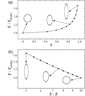
Figure 5: The effective force between two ellipses in terms of (a) the eccentricity $\epsilon$, and (b) the small radius of the ellipses $b$. The distance between the centers of the intruders is fixed at $D\!_{{}_{\text{AB}}}{=}30R$, and the forces are scaled by the force between two circles.

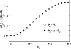
Figure 6: The effective force between the ellipses vs. the angle $\theta_{\!{}_{A}}$. The forces are scaled by the force at $\theta_{\!{}_{A}}{=}0$.

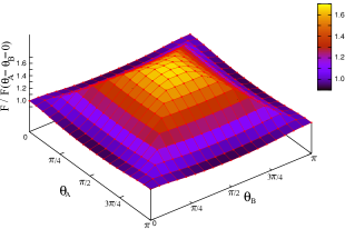
Figure 7: (color online) The force between two ellipses in terms of the angles $\theta_{\!{}_{A}}$ and $\theta_{\!{}_{B}}$. The color intensity reflects the magnitude of $F$.

Let us first fix the orientation of the ellipses at $\theta_{\!{}_{A}}{=}\theta_{\!{}_{B}}{=}\pi{/}2$ and the distance between their centers at $D\!_{{}_{\text{AB}}}{=}30R$. We modify the shape of intruders by changing the ratio between the ellipse radii, $a{/}b$, while its area is constant, i.e. $\pi ab{=}100\pi R^{2}({=}\pi R_{\!{}_{I}}^{2})$. The deviation of the shape from being circular can be characterized with the eccentricity parameter defined as

$$\epsilon=\sqrt{1-\displaystyle\frac{b^{2}}{a^{2}}}.$$ (32)

Using the same procedure as in Sec. III we calculate the effective force between two ellipses as $F{=}\int_{-a}^{a}\Delta p(y)dy$. Figure 5 shows that the force considerably increases as the shape further deviates from being circular. The behavior of $F$ results from two competing effects: first, increasing $\epsilon$ causes lower pressure difference because $D\!_{{}_{\text{out}}}{/}D\!_{{}_{\text{in}}}$ decreases on average; second, it also increases the integration interval $[-a,a]$, which increases the force. The latter effect seems to be more important so that the force monotonically increases with $\epsilon$.

Next we investigate the influence of the orientations of the ellipses on the fluctuation-induced force. One expects that the eccentricity of the elliptical intruders also influences the force behavior when the orientation changes. Only in the limit of circular shapes the orientation plays no role anymore. Therefore, we fix the shape by choosing $a{=}2b{=}10R$ and vary the angles $\theta_{\!{}_{A}}$ and $\theta_{\!{}_{B}}$. Let us first consider two cases $\theta_{\!{}_{A}}{=}\theta_{\!{}_{B}}$ and $\theta_{\!{}_{A}}{=}\pi{-}\theta_{\!{}_{B}}$ for simplicity, thus, there remains only one rotational degree of freedom. The force is given by

$$F{=}\int_{-y_{{}_{\text{max}}}}^{y_{{}_{\text{max}}}}\Delta p(y)dy,$$ (33)

where the interval [$-y_{{}_{\text{max}}},y_{{}_{\text{max}}}$] is the range of $y$ coordinate covered by both intruders. In the case of $\theta_{A}{\neq}\theta_{B}$, each intruder covers a different range of $y$ coordinate, leading to a different value of $y_{{}_{\text{max}}}$. Thus, in general, we choose the smaller value of $y_{{}_{\text{max}}}$ to calculate the integral, i.e. only the area where two elliptical intruders face each other is taken into account

$$y_{{}_{\text{max}}}=\text{min}\Big{(}\displaystyle\frac{c_{{}_{1}}}{\displaystyle\sqrt{c_{{}_{1}}^{2}c_{{}_{2}}-c_{{}_{3}}^{2}c_{{}_{1}}}},\displaystyle\frac{c_{{}_{4}}}{\displaystyle\sqrt{c_{{}_{4}}^{2}c_{{}_{5}}-c_{{}_{6}}^{2}c_{{}_{4}}}}\Big{)}.$$ (34)

With increasing the angle $\theta_{\!{}_{A}}$, on the one hand the average ratio $D\!_{{}_{\text{out}}}{/}D\!_{{}_{\text{in}}}$ decreases which weakens the pressure difference between the gap and outside regions. On the other hand, the integration interval $[-y_{{}_{\text{max}}},y_{{}_{\text{max}}}]$ is extended which increases the force. Figure 6 shows that the intruders exert stronger forces on each other in the case $\theta_{\!{}_{A}}{=}\theta_{\!{}_{B}}{=}\pi/2$ (maximum area, minimum $\Delta p$) compared with $\theta_{\!{}_{A}}{=}\theta_{\!{}_{B}}{=}0$ (minimum area, maximum $\Delta p$). One can also see that the interaction in the case of $\theta_{\!{}_{A}}{=}\pi{-}\theta_{\!{}_{B}}$ is slightly stronger than the case $\theta_{\!{}_{A}}{=}\theta_{\!{}_{B}}$ (except at $\theta_{\!{}_{A}}{=}0,\pi/2$). The results of the general case of $\theta_{\!{}_{A}}{\neq}\theta_{\!{}_{B}}$ are shown in Fig. 7. The configuration with $\theta_{\!{}_{A}}{=}\theta_{\!{}_{B}}{=}\pi/2$ produces the strongest interaction, while the lowest force is obtained if $|\theta_{\!{}_{A}}{-}\theta_{\!{}_{B}}|{=}\pi/2$ and $\theta_{\!{}_{A}}{=}\pi/2$ (or $\theta_{\!{}_{B}}{=}\pi/2)$. Therefore, the maximum fluctuation-induced force is obtained when the two ellipses are aligned along the $y$ axis. This result, however, can not be trivially extended to more complicated situations, and a comprehensive study is required to elucidate the role of key parameters such as gas density and restitution coefficient, as well as the number, position, and orientation of the intruders in a multi-body configuration.

VI Discussion and Conclusion

We reviewed the detailed calculations of the mode coupling method to describe the nonequilibrium steady state of a randomly driven granular system. When the existence of arising long-range hydrodynamic correlations (reflected in the structure factors) is accompanied by geometric constraints, effective long-range forces appear. Using the pair correlation functions in the mode coupling calculations leads to a reasonable estimation of the force between two intruders. It is notable that the hydrodynamic correlations become stronger in multi-intruder configurations or binary mixtures, which necessitates the usage of triplet or higher order structure factors Shaebani12 ; Dijkstra06 . The validity of the hydrodynamic description is also limited to large restitution coefficients. The steady state of an inelastic granular fluid is inhomogeneous, resulting in a length scale $l_{i}$ on which the macroscopic hydrodynamic fields vary. Decreasing the restitution coefficient would increase the gradient of the inhomogeneities, i.e. decreases the length scale $l_{i}$. The hydrodynamic description of the system holds only when $l_{i}$ is well separated from the mean-free path $l^{*}$ of the granular gas, and this happens only for large restitution coefficients.

Another point is that the analytical results presented in this work are restricted to two dimensions but the procedure can be extended to three dimensions e.g. by considering a suitable equation of state for hard sphere systems, and calculating the force exerted on the surface of three-dimensional obstacles. Nevertheless, the behavior of pressure fluctuations is different in two and three dimensions (it behaves as $1/r$ in 3D while diverges logarithmically as $\text{ln}(L/r)$ in 2D). Thus, the force is independent of (logarithmically dependent on) the system size in three (two) dimensions Shaebani12 . Indeed, the long-range behavior of the correlations and the dimensional dependence of the effective force originate from the behavior of the inverse of the Laplacian in the hydrodynamic equations vanNoije99 .

Finally, we have shown that changing the shape or orientation of the intruders influences the effective force in two different ways: (i) by modifying the gap length (along the $x$-direction), which affects the pressure difference around the intruders, (ii) by modifying the gap width (along the $y$-direction) which changes the force integration interval. The spatial correlations decay rather slowly, meaning that tiny changes in the boundary conditions can not dramatically influence the pressure difference and, thus, the force. Still, there might be a visible impact on the effective force, since varying the particle elongation in the $y$-direction strongly changes the area on which the force is applied.

References

- (1) P. K. Haff, J. Fluid Mech. 134, 401 (1983).
- (2) R. Brito and M. H. Ernst, Europhys. Lett. 43, 497 (1998).
- (3) I. Goldhirsch and G. Zanetti, Phys. Rev. Lett. 70, 1619 (1993).
- (4) E. Efrati, E. Livne, and B. Meerson, Phys. Rev. Lett. 94, 088001 (2005).
- (5) C. Cattuto and U. M. B. Marconi, Phys. Rev. Lett. 92, 174502 (2004).
- (6) D. R. M. Williams and F. C. MacKintosh, Phys. Rev. E 54, R9 (1996).
- (7) G. Peng and T. Ohta, Phys. Rev. E 58, 4737 (1998).
- (8) T. P. C. van Noije, M. H. Ernst, E. Trizac, and I. Pagonabarraga, Phys. Rev. E 59, 4326 (1999).
- (9) L. Oger, C. Annic, D. Bideau, R. Dai, and S. B. Savage, J. Stat. Phys. 82, 1047 (1996).
- (10) T. P. C. van Noije, M. H. Ernst, R. Brito, and J. A. G. Orza, Phys. Rev. Lett. 79, 411 (1997).
- (11) M. Otsuki and H. Hayakawa, Phys. Rev. E 79, 021502 (2009).
- (12) H. B. G. Casimir, Proc. K. Ned. Akad. Wet. 51, 793 (1948).
- (13) M. Kardar and R. Golestanian, Rev. Mod. Phys. 71, 1233 (1999).
- (14) S. Aumaitre, C. A. Kruelle, and I. Rehberg, Phys. Rev. E 64, 041305 (2001).
- (15) I. Zuriguel, J. F. Boudet, Y. Amarouchene, and H. Kellay, Phys. Rev. Lett. 95, 258002 (2005).
- (16) Y. Y. Villanueva, D. V. Denisov, S. de Man, and R. J. Wijngaarden, Phys. Rev. E 82, 041303 (2010).
- (17) L. A. García-Trujillo et al., arXiv:1212.3202.
- (18) N. Rivas et al., Phys. Rev. Lett. 106, 088001 (2011).
- (19) D. A. Sanders, M. R. Swift, R. M. Bowley, and P. J. King, Phys. Rev. Lett. 93, 208002 (2004).
- (20) D. V. Denisov, Y. Y. Villanueva, and R. J. Wijngaarden, Phys. Rev. E 83, 061301 (2011).
- (21) C. Cattuto, R. Brito, U. M. B. Marconi, F. Nori, and R. Soto, Phys. Rev. Lett. 96, 178001 (2006).
- (22) M. R. Shaebani, J. Sarabadani, and D. E. Wolf, Phys. Rev. Lett. 108, 198001 (2012).
- (23) P. R. Buenzli, J. Phys. Conf. Ser. 161 012036 (2009).
- (24) S. Asakura and F. Oosawa, J. Chem. Phys. 22, 1255 (1954).
- (25) G. Gradenigo, A. Sarracino, D. Villamaina, and A. Puglisi, J. Stat. Mech. 08, P08017 (2011).
- (26) S. Chapman and T. G. Cowling, The Mathematical Theory of Non-uniform Gases (Cambridge University Press, Cambridge, 1970).
- (27) L. Verlet and D. Levesque, Mol. Phys. 46, 969 (1982).
- (28) T. P. C. van Noije and M. H. Ernst, Phys. Rev. E 61, 1765 (2000).
- (29) L. Landau and E. M. Lifshitz, Fluid Mechanics (Pergamon Press, New York, 1959).
- (30) D. Bartolo, A. Ajdari, J. B. Fournier, and R. Golestanian, Phys. Rev. Lett. 89, 230601 (2002).
- (31) M. Dijkstra et al., Phys. Rev. E 73, 041404 (2006).