Properties of Star Clusters - I: Automatic Distance and Extinction Estimates

Abstract

Determining star cluster distances is essential to analyse their properties and distribution in the Galaxy. In particular it is desirable to have a reliable, purely photometric distance estimation method for large samples of newly discovered cluster candidates e.g. from 2MASS, UKIDSS-GPS and VISTA-VVV. Here, we establish an automatic method to estimate distances and reddening from NIR photometry alone, without the use of isochrone fitting. We employ a decontamination procedure of JHK photometry to determine the density of stars foreground to clusters and a galactic model to estimate distances. We then calibrate the method using clusters with known properties. This allows us to establish distance estimates with better than 40 % accuracy.

We apply our method to determine the extinction and distance values to 378 known open clusters and 397 cluster candidates from the list of Froebrich, Scholz and Raftery (2003). We find that the sample is biased towards clusters of a distance of approximately 3 kpc, with typical distances between 2 and 6 kpc. Using the cluster distances and extinction values, we investigate how the average extinction per kiloparsec distance changes as a function of Galactic longitude. We find a systematic dependence that can be approximated by $A_{H}(l)$ [mag/kpc] = 0.10 + 0.001$\times\left|l-180^{\circ}\right|/^{\circ}$ for regions more than 60^∘ from the Galactic Centre.

1 Introduction

Star clusters are the building blocks of the Galaxy and act as tracers of stellar and Galactic evolution. With the large fraction of stars in the Milky Way formed in star clusters (e.g. Lada & Lada (2003)), it is important to determine fundamental properties of clusters such as age, reddening and mass. Determination of distance is essential to analyse these properties and the distribution of clusters throughout the Galaxy.

When a large sample of clusters is available, objects of interest such as massive clusters and old clusters near the Galactic Centre (GC, see e.g. Bonatto & Bica (2007a)), become available to study. Large cluster candidate samples, such as the list based on data from the 2 Micron All Sky Survey (2MASS) by Froebrich et al. (2007) (FSR hereafter) and others (e.g. Borissova et al. (2011), Chené et al. (2012)) have become readily available in recent years. Further samples are forthcoming from large scale Near Infrared (NIR) surveys such as the UK Infrared Deep Sky Survey (UKIDSS) Galactic Plane Survey (GPS, Lucas et al. (2008)) and the VISTA-VVV survey (Minniti et al., 2010). Here we aim to establish an automatic method to estimate distances and reddening for such large cluster candidate samples from NIR photometry alone without the use of, or to be used as starting point for, isochrone fitting.

In a forthcoming paper (Paper II) we will extend our work and determine the ages of all clusters. We will also improve the accuracy of the distances and extinction estimates from this paper by means of isochrone fitting. That will provide us with the ability to characterise and analyse the general properties of the entire FSR sample and to investigate the distribution of ages, reddening and distances as well as their spatial distribution, observational biases and evolutionary trends. It will also allow us to extract the best massive cluster candidates amongst the FSR sample.

This paper is structured as follows. In Section 2 we discuss our selections of 2MASS$/$WISE data and describe in detail our foreground star counting technique as a distance estimator. We then introduce and detail our distance calibration and optimisation method in Section 2.5. In Section 3 we discuss the results of our calibration and optimisation method applied to the FSR list of cluster candidates and the extinction $A_{H}$ per kpc measurement as a function of Galactic longitude.

2 Analysis Methods

In the following section we will detail our homogeneous and automated approach to estimate and calibrate distances and extinction values for all FSR clusters, based on photometric archival data. Our suggested method can be applied to any large sample of star clusters and cluster candidates containing a sufficient number of objects with known distances (which will be used as calibrators).

2.1 2MASS/WISE Data and Cluster Radii

Our distance and extinction estimates will rely on identifying the colour of the most likely cluster members. For this purpose we will determine a membership-likelihood or photometric cluster membership probability for every star in each cluster (see Sect. 2.2). As a first step we hence need to specify the area around the cluster which contains most cluster members, as well as an area near the cluster which will be used as control field.

For this purpose we use the coordinates of all FSR clusters as published in Froebrich et al. (2007). Note that this paper only contains the coordinates of the 1021 newly discovered cluster candidates. The positions of the remaining 681 previously known open clusters and 86 globular clusters are not published. For each FSR cluster we extract near infrared JHK photometry from the 2MASS (Skrutskie et al., 2006) point source catalogue. All sources within a circular area of $0.5^{\circ}$ radius around the cluster coordinates are selected, as long as the photometric quality flag (Qflg) was better than ”CCC”. Typically, between 50 % and 70 % of all stars in the catalogue have a Qflg better than ”CCC” (C-sample, hereafter). Furthermore, about 35 % to 45 % of all stars have a Qflg of ”AAA” (A-sample, hereafter), i.e. are of the highest photometric quality. Thus, the C-sample contains on average about 1.5 times as many stars as the A-sample.

For each cluster we use the C-sample to fit a radial star density profile of the form:

$$\rho(r)=\rho_{bg}+\rho_{cen}\left[1+\left(\frac{r}{r_{cor}}\right)^{2}\right]^{-1}$$ (1)

Where $r_{cor}$ is the cluster core radius, $\rho(r)$ the star density as a function of distance $r$ from the cluster centre, $\rho_{bg}$ the (assumed constant) background star density and $\rho_{cen}$ the central star density above the background of the cluster.

We define as cluster area ($A_{cl}$) everything in a circular area around the cluster centre within $F$ times the cluster core radius. In our subsequent analysis we will vary the value of $F$ between one and three. The control area ($A_{con}$) for each cluster will be a ring around the cluster centre with an inner radius of five times $r_{cor}$ and an outer radius of $0.5^{\circ}$.

Note that the star density profile used has no tidal radius and thus in principle results in an infinite number of cluster stars. However, if we assume that outside five core radii (the control field) there are no member stars, then the region within three core radii contains about 70 % of all cluster members. If all cluster stars are contained within three core radii, then 70 % of the cluster members are found closer than two core radii from the centre.

In additional to the 2MASS Near Infrared photometry, we also utilise mid infrared data from the WISE satellite in order to estimate the colour excess of cluster stars and hence the extinction (see Sect. 2.8). We obtain all sources from the WISE all-sky catalogue (Wright et al., 2010) within three times the cluster core radius. The WISE all-sky catalogue is cross-matched to 2MASS, hence we can easily identify the stars in both, the A- and C-sample, that have a WISE counterpart.

2.2 Photometric Cluster Membership Probabilities

In order to estimate the typical colour of cluster members for our analysis, as well as to identify potential foreground and background stars to determine the distance, we require some measure of membership-likelihood for every star in a cluster. We base our calculation on the well established NIR colour-colour-magnitude (CCM) method outlined in e.g. Bonatto & Bica (2007b) and references therein. Based on earlier simulations, e.g. in Bonatto et al. (2004), Bonatto & Bica (2007b) note that using the J-band magnitude, as well as the J-H and J-K colours from 2MASS photometry, provides the maximum variance among cluster colour-magnitude sequences for open clusters of different ages. Since our sample will most likely contain clusters of all ages, we thus use the same colours for our analysis.

All confirmed clusters and cluster candidates in the FSR list are selected as spatial overdensities. Our photometric cluster membership probabilities are based on ’local’ overdensities in the above mentioned CCM space. Thus, we need to establish where these overdensities are in CCM space and if these overdensities are in agreement with the expectation for a real star cluster. Bonatto & Bica (2007b) use a small cuboid in CCM space to determine the overdensities and the related photometric membership probabilities, where the dimension of the J-magnitude side length of the cuboid is larger than the side length of the colours. Instead of a small cuboid, Froebrich et al. (2010) use a small prolate ellipsoid in the specified CCM space, where the dimensions along the J-band magnitude are larger than along the colours. Note that the actual shape used to determine the local overdensity in CCM space (cuboid, ellipsoid, or else) is unimportant for the identification of the most likely cluster members.

Thus, for each cluster we determine the photometric cluster membership probability for every star using the method described below. Following Froebrich et al. (2010) we determine the CCM distance, $r_{ccm}$, between the star, $i$, and every other star $j\neq i$ in the cluster area using:

$$r_{ccm}=\sqrt{\frac{1}{2}\left(J_{i}-J_{j}\right)^{2}+\left(JK_{i}-JK_{j}\right)^{2}+\left(JH_{i}-JH_{j}\right)^{2}}$$ (2)

Where $JK=J-K$ and $JH=J-H$ are the Near Infrared colours from 2MASS for all stars. We denote with $r^{N}_{ccm}$ the CCM distance of star $i$ to the $N^{th}$ nearest neighbour in CCM space. Froebrich et al. (2010) used $N=10$ to investigate old star clusters amongst the FSR sample. However, it is not formally established which value for $N$ gives the best results for our purpose. We hence vary $N$ from 10 to 30 and investigate the influence of the value on the distance calibration in Sect. 2.6. The value of $N$ essentially defines, in conjunction with the total number of stars in the cluster area, the resolution at which we can separate potential cluster members from field stars in CCM space. Increasing $N$ will degrade the resolution and thus e.g. widen any potential cluster Main Sequence. Using smaller values for $N$ will increase the resolution, but will at the same time decrease the signal to noise ratio of the determined photometric cluster membership probabilities. Our range of values for $N$ is hence a compromise between resolution and signal to noise ratio. Note, that the typical number of stars in the cluster area for our objects is between 100 and 300 for the A-sample. Thus, our resolution in CCM space varies by less than a factor of $1.5$ between clusters.

We then determine the CCM distance of all stars in the cluster control field to star $i$ in the same way as for the cluster area. $N^{con}_{ccm}$ is then the number of stars closer than $r^{N}_{ccm}$ to star $i$ in the control field. If both $N$ and $N^{con}_{ccm}$ are normalised by their respective area on the sky, one can calculate a membership-likelihood index of star $i$, $P^{i}_{cl}$ as:

$$P^{i}_{cl}=1.0-\frac{N^{con}_{ccm}}{N}\frac{A_{cl}}{A_{con}}.$$ (3)

Due to statistical fluctuations in the number of field stars in the control and cluster area, the above equation can in principle lead to negative values. We thus set any negative $P^{i}_{cl}$ value to zero and note that $P^{i}_{cl}$ is in principle not a real membership probability. However, all we require is a list of the most likely cluster members, which are reliably identified by this method. Note that after our calibration (see Sect. 2.5.3) the sum of all $P^{i}_{cl}$ values equals the total excess of stars in the cluster field compared to the control field. Furthermore, the sum all $1-P^{i}_{cl}$ values equals the number of field stars. Thus, this membership-likelihood index can be treated as a probability. Hence we will refer to $P^{i}_{cl}$ as the photometric cluster membership probability of star $i$ hereafter.

In principle one could combine the above described colour based membership probabilities with spatial information. In other words one could determine a probability $P^{i}_{pos}$ based on the distance of the star to the cluster centre as well as the background and cluster star density determined via Eq. 1.

$$P^{i}_{pos}=\frac{\rho_{cen}}{\rho_{bg}}\left[1+\left(\frac{r}{r_{cor}}\right)^{2}\right]^{-1}$$ (4)

Following Froebrich et al. (2010), we refrain from applying this method for several reasons:

i) In dense clusters the probabilities are unreliable due to crowding near the centre.

ii) For clusters projected onto a high background density of stars the $P^{i}_{pos}$ values tend to be very low. This makes the cluster not stand out from the background stars in many cases, even if cluster stars have very different colours compared to the field population.

iii) Our sample will contain a number of young clusters which do not appear circular in projection. Thus, the position dependent membership probabilities cannot be determined by Eq. 4.

We hence only use the $P^{i}_{cl}$ values to identify the most likely cluster members.

Note that the individual photometric cluster membership probabilities are a function of the ’free’ parameters in our approach. Hence, $P^{i}_{cl}$ will depend on the sample of stars (A- or C-sample) used, the cluster area $A_{cl}$ (between one and three cluster core radii), and the nearest neighbour $10\leq N\leq 30$ chosen in the CCM distance calculation. We will discuss this in detail in Sect. 2.6.

As an example of how our method performs, we show in Fig. 1 several diagrams for the cluster FSR 0233. Different coloured symbols in the graphs indicate the various photometric cluster membership probabilities for the stars determined for the A-sample within two cluster core radii and for $N=15$. The top row shows the Colour-Colour Diagram (CCD, left) and Colour-Magnitude Diagram (CMD, right) of the cluster region. In the CMD one can clearly identify that the high probability cluster members form the top of a Main Sequence and a clump of red giants, suggesting an older cluster. Indeed, this is the known open cluster LK 10, which is about 1 Gyr old and relatively massive (Bonatto & Bica, 2009). In the bottom panels we show the spatial distribution of the cluster stars. In the left panel we only include stars with a membership probability above 60 %, while in the right panel we only plot the remaining low probability members. One can clearly see that the low probability members, which are the most likely field stars, are distributed homogeneously in the field. In the left panel one can identify an increase in the density of stars, slightly off-centre, that indicates the cluster centre.

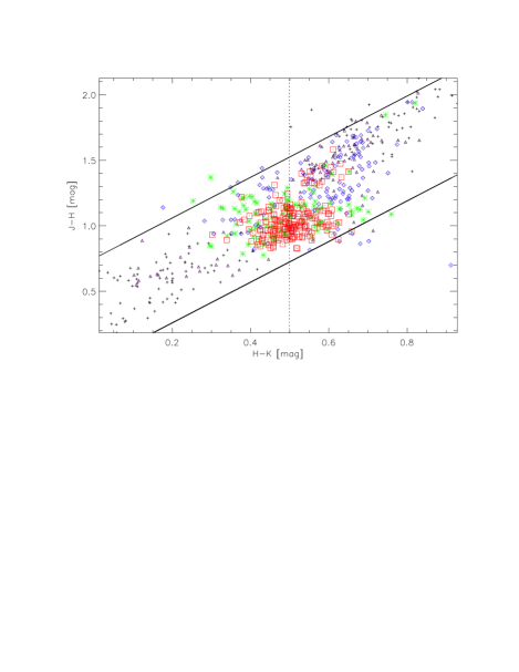
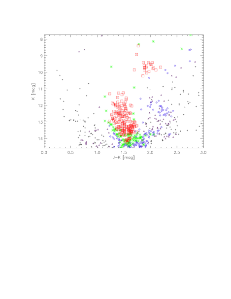
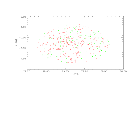
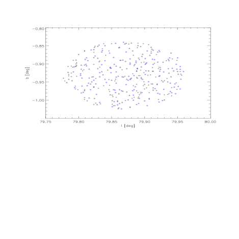
Figure 1: Diagrams of all A-sample stars within two cluster core radii for FSR 0233. The various symbols represent the cluster membership probabilities determined for $N=15$: $P^{i}_{cl}>80\%$ red squares; $60\leq P^{i}_{cl}<80\%$ green stars; $40\leq P^{i}_{cl}<60\%$ blue diamonds; $20\leq P^{i}_{cl}<40\%$ purple triangles; $P^{i}_{cl}<20\%$ black plus signs. The top row contains the colour-colour (left) and colour-magnitude diagram (right). The vertical solid line in the left panel represents the $HK_{med}$ value (0.50 mag) determined for the cluster (see text for details). In the bottom row we plot the positions of the stars with a photometric membership probability of more (left) and less (right) than 60 %.

2.3 Identification of Foreground Stars

For our distance calculation it is not sufficient to solely identify the most likely cluster members. We further need to establish the most likely foreground stars to the cluster.

We utilise the median colour of the stars with the highest cluster membership probability to separate foreground and background objects. The notion is that stars bluer than the median colour of the cluster members are likely to be foreground and objects redder than this are most likely in the background.

The combination of 2MASS and WISE allows us, in principle, to use a variety of colours for this selection. However, ideally the colour with the smallest spread amongst the spectral types and luminosity classes should be used, since any reddening can then be attributed to interstellar extinction. The ideal choice would be the difference between the 2MASS H-band and the 4.5 $\mu$m WISE band ($H-[4.5]$), since its intrinsic value is almost independent of spectral type and/or luminosity class (Majewski et al., 2011). However, due to the low spatial resolution of WISE, only a fraction of all 2MASS sources in each cluster are actually detected unambiguously in $[4.5]$. We hence, use ($H-K$) for the purpose of foreground star selection, but refer back to ($H-[4.5]$) in the extinction determination (see Sect. 2.8).

For every cluster we arrange the individual photometric cluster membership probabilities, $P^{i}_{cl}$, in descending order. The median ($H-K$) of the top 25 % – 45 % of the highest probability members is calculated in 5 % increments. We then define $HK_{med}$ as the median of these five ($H-K$) values, to represent the most likely ($H-K$) colour of the cluster stars. All stars in the cluster area with an ($H-K$) value equal to, or greater than, $HK_{med}$ are considered redder than the cluster and are hence potential background stars. All stars with an ($H-K$) value less than $HK_{med}$ are considered bluer than the cluster, and hence can be potential foreground objects. Based on this, we determine the number density of foreground stars, $\rho^{cl}_{fg}$, projected onto the cluster as the sum of all non-membership probabilities of the potential ’blue’ foreground stars:

$$\rho^{cl}_{fg}=\frac{1}{A_{cl}}\sum\limits_{i,blue}{\left(1.0-P^{i}_{cl}\right)}$$ (5)

We note that for particular cases, where cluster members are intrinsically red, such as embedded clusters, or clusters behind multiple layers of foreground extinction, this method will not lead to the correct number of foreground stars. The same applies if there are intrinsically hot/blue stars in the cluster area. Furthermore, photometric scatter will influence the number of blue objects. However, our calibration procedure (see Sect. 2.5) will statistically adjust for this.

2.4 Determination of Cluster Distances

The above determined projected number density of foreground stars towards each cluster can be used to estimate the distance, by comparing this number to predictions from models for the distribution of stars within the Galaxy. Our model of choice is the Besançon Galaxy Model (BGM) by Robin et al. (2003) and we utilise its web interface to simulate the foreground population of stars towards all our clusters.

We use the default settings of the BGM. i.e. no clouds and 0.7 mag of optical extinction per kiloparsec distance. The photometric limits (completeness limit and photometric uncertainties as a function of brightness) in the 2MASS JHK filters are determined for each cluster and sample (A and C) separately in the control field area. After initial tests with the above settings, we perform simulations for each cluster position for an area large enough to contain a total of about 5000 simulated stars. This ensures that the uncertainties of our inferred distances are not dominated by the random nature (or small number statistics) in the model output.

The list of stars returned by the BGM simulation for the field of the cluster is sorted by distance. With the known area of the simulation, we are hence able to determine up to which distance model stars need to be considered to result in a model star density equal to our determined foreground density for the cluster. Henceforth, we will refer to this distance to the cluster as the Model Distance, $d_{mod}$.

Figure 2: Left: Histogram of the age distributions of CCS 1 – old FSR clusters. Right: Histogram of the age distributions of CCS  2 – WEBDA counterparts of FSR clusters.

2.5 Calibration of Cluster Model Distances

The model distances determined above are not necessarily accurate without further calibration. Foster et al. (2012) have shown that distances estimated from foreground star counts to dark clouds with maser sources agree with maser parallax measurements in most cases. Ioannidis & Froebrich (2012) have used a similar approach to us to measure distances to dark clouds with jets and outflows. They used objects of known distances from the Red MSX Source (RMS, MSX - Midcourse Space Experiment) survey by Urquhart et al. (2008) to calibrate their distances, which resulted in an accuracy for the distances that resembled the intrinsic scatter of the calibration objects.

For the FSR star cluster (candidates) the situation is more complex. Typically the objects are not associated with dark clouds, hence the separation of foreground and background objects (via median NIR colours) is less certain. Furthermore, crowding in the cluster (and partly even in the control field) will influence the observed foreground star density. Finally, it is unclear which parameter values used to determine the model distance $d_{mod}$, lead to the most accurate results.

Thus, we use sets of calibration samples of star clusters, a number of corrections to the observed foreground star density and a parameter study to investigate the accuracy of our method. In the following section we detail our calibration approach.

2.5.1 Cluster Calibration Samples

As in Ioannidis & Froebrich (2012), we aim to have a Cluster Calibration Sample (CCS) that consists of objects of a similar nature to the targets whose distance we are aiming to determine. Hence, ideally we would use a sub-set of the FSR clusters which have accurately determined distances.

There are three obvious choices: i) CCS 1 – The sample of old open FSR clusters investigated by Froebrich et al. (2010); ii) CCS 2 – known FSR clusters that have a counterpart in the WEBDA database by Mermilliod (1995); iii) CCS 3 – FSR cluster counterparts with distances in the online version of the list of star clusters from Dias et al. (2002).

All three of these samples have their obvious disadvantages. Both CCS 2 and CCS 3 are constructed from literature searches. The cluster distances in these samples are determined by various methods and are hence inhomogeneous. Thus, it is impossible to estimate the intrinsic scatter of the distances of the sample clusters. CCS 1, on the other hand, has homogeneously determined distances (with a 30 % scatter, Froebrich et al. (2010)) but consists almost exclusively of old star clusters. The full FSR sample, however, should contain a mix of young, intermediate age and old objects and it is unknown if there are systematic differences if our method is applied to clusters of different ages.

Thus, we use two of the cluster samples to test and calibrate our distance calculation method: i) CCS 1 – the old FSR clusters from Froebrich et al. (2010); ii) CCS 2 – the FSR counterparts in WEBDA, since this catalogue generally includes only high accuracy measurements compared to the list from Dias et al. (2002), which is more complete.

i) The old FSR sample contains 206 old open clusters. We remove every object that is a suspected globular cluster (e.g. FSR 0190 Froebrich et al. (2008) and FSR 1716 Froebrich et al. (2008)), which has less than 30 stars within one core radius, and/or less than 30 stars in the control field (the latter two conditions are for the A-sample of stars). We also remove any cluster with a core radius of more than 0.05^∘. This selection leaves 115 old open clusters in the CCS 1 sample.

ii) We cross-match the entire FSR list with all entries in WEBDA. We consider the objects as a match, if there was exactly one counterpart within 7.5′. In the case where two FSR objects are near the same WEBDA entry the objects are removed. We also require that every WEBDA match has a distance, age and reddening value. Finally, as for CCS 1, we remove objects with less than 30 stars within one core radius, less than 30 stars in the control field (for the A-sample of stars) and a core radius of more than 0.05^∘. The final CCS 2 sample after these selections contains 241 clusters.

The two CCSs have different properties which we will briefly discuss here. The majority of clusters in CCS 1 are between 1 and 4 kpc distance, but there are a number of objects that are up to 8 kpc or further away. In contrast, CCS 2 contains mostly clusters which are less than 3 kpc distant, with very few objects more than 5 kpc away. The reddening distribution of CCS 1 is biased towards low A_V clusters. The number of objects declines steeply with increasing extinction, and there are almost no clusters with A${}_{V}>$ 4 mag. The CCS 2, on the other hand, has a homogeneous distribution of A_V values between 0 and 3 mag. Again, high extinction clusters are rare in the sample. However the biggest difference between the two samples of calibration clusters is the age distribution (see Fig. 2). While in CCS 1 almost all clusters are about 1 Gyr old (within a factor of a few), CCS 2 shows a more homogeneous distribution of ages between 10 Myrs and a few Gyrs.

2.5.2 Measuring Calibration Accuracy

To quantify how well our method estimates the cluster distances for the different CCSs we use the logarithmic distance ratio defined for each cluster as:

$$R=\log_{10}\left(\frac{d_{lit}}{d_{mod}}\right)$$ (6)

Where $d_{lit}$ is the cluster distance as obtained from the literature and $d_{mod}$ the distance determined from the foreground star density and the BGM. If the value of $R$ is positive, then our our method underestimates the cluster distance, if $R$ is negative, we overestimate the distance. We determine the $rms$ of the distribution of $R$ values for each CCS and use this as a measure for the scatter $S=(10^{rms}-1)$ of our method.

2.5.3 Crowding and Extinction Correction

There are a number of factors that we use to determine the model distance to the cluster which will alter the measured foreground star density (see Sect. 2.3). These are large scale foreground extinction and crowding (in the general field and the centre of the cluster). Both effects are not considered by the BGM, but can in principle be corrected for.

If there is large scale foreground extinction in the direction of the cluster, the BGM will essentially predict a higher star density ($\rho_{BGM}$) than the one we measure in the control field ($\rho_{con}$) around the cluster. Similarly, close to the Galactic Plane and in particular near the Galactic Centre, crowding becomes a major factor for the number of detected stars in 2MASS. Again, the star density predicted by the BGM will be larger compared to the measured value in our control field. Thus, to correct for both effects simultaneously, we multiply the measured foreground star density $\rho^{cl}_{fg}$ by a factor:

$$X_{1}=\frac{\rho_{BGM}}{\rho_{con}}$$ (7)

Furthermore, crowding will be increased in the area of the cluster, since there are naturally more stars in that region. The effect this has can be estimated, since the observed star density in the control area should be equal to the density of non-cluster stars in the cluster area. The latter can be easily determined by summing up the non-membership probabilities of all stars in the cluster area and dividing by $A_{cl}$. Thus, correcting the measured foreground star density by another factor will correct for the additional crowding in the cluster area compared to the control field:

$$X_{2}=\frac{\rho_{con}\times A_{cl}}{\sum\limits_{i}\left(1.0-P^{i}_{cl}\right)}$$ (8)

This factor also addresses related differences in the completeness limit which is used in the BGM simulation for the cluster, but has been estimated in the control area.

In summary, to estimate the model distance for the clusters via the BGM we will use the corrected foreground star density $\rho^{cl,cor}_{fg}$ which is determined as:

$$\rho^{cl,cor}_{fg}=X_{1}\times X_{2}\times\rho^{cl}_{fg}=\frac{\rho_{BGM}\times A_{cl}}{\sum\limits_{i}\left(1.0-P^{i}_{cl}\right)}\times\rho^{cl}_{fg}$$ (9)

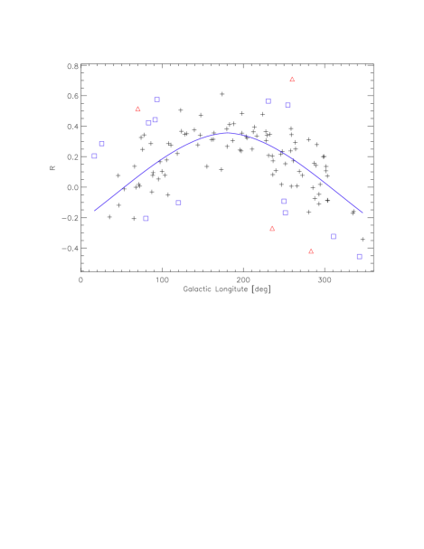
Figure 3: Plot of $R$ vs. the Galactic longitude of the CCS 1 objects. These are based on distance calculations using the A-sample, a cluster radius of $1\times r_{cor}$ and a nearest neighbour number in the photometric decontamination of $N=25$. The solid line indicates our 3rd order polynomal fit. Black cross’ represent points used for the fit with $2\sigma$ clipping, blue squares represent clusters that were excluded at the $2\sigma$ level and red triangles represent clusters excluded at the $3\sigma$ level.

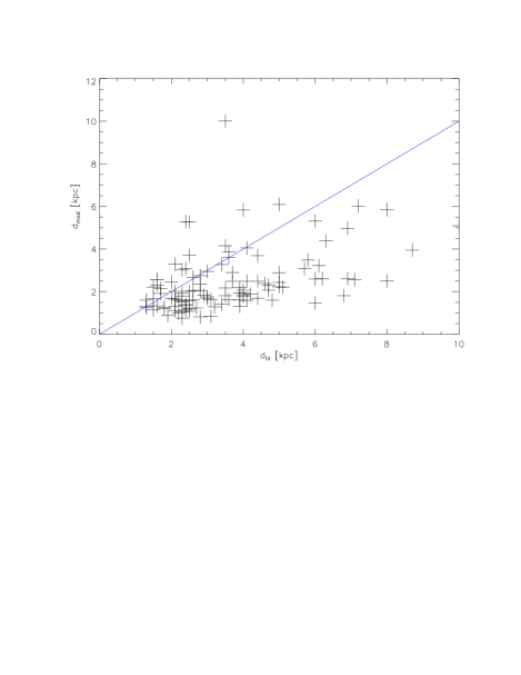
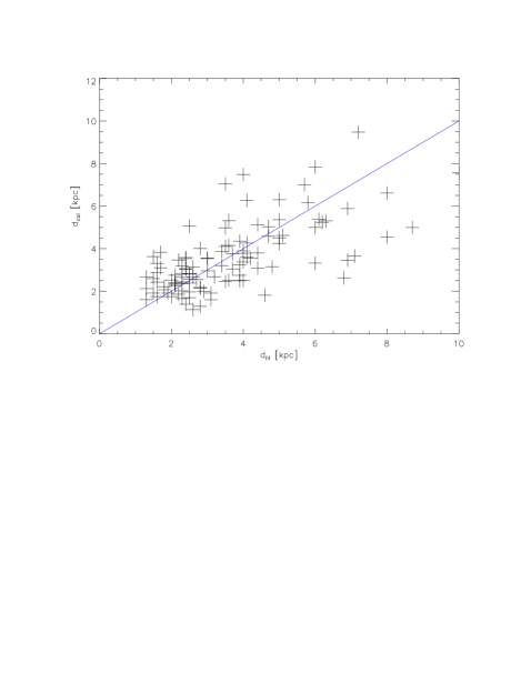
Figure 4: Example plot of the literature distances $d_{lit}$ for CCS 1 clusters (black crosses) against our uncalibrated model distance $d_{mod}$ (left) and the calibrated model distances $d_{cal}$ (right). The calibration used the A-sample, a nearest neighbour in the photometric decontamination of $N=25$ and a radius of $1\times r_{cor}$. We overplot the 1:1 line in both cases. The final scatter $S_{cal}$ corresponds to a 40 % uncertainty in the calibrated distances.

2.5.4 Position Dependent Corrections

With the observed foreground star density corrected for crowding and large scale extinction, we can estimate the model distance, $d_{mod}$, and compare to the literature distance, $d_{lit}$, of the CCSs to investigate the scatter $S$ of the distribution of the logarithmic distance ratios for all clusters in each CCS.

We investigate if there are any obvious correlations of the value of $R$ with cluster parameters that are known or can be estimated for every cluster (candidate) in the FSR sample. These include the Galactic Position ($l$ and $b$), the apparent radius, the control field star density and the extinction (based on $HK_{med}$, see Sect. 2.3).

A significant trend occurs with the Galactic longitude. This can be seen in Fig. 3. There a clear underestimate of the cluster distances towards the Galactic Anticentre is apparent, while closer to the Galactic Centre our method overestimates the distances. We find that a simple 3^rd order polynomial fit can be used to correct this trend and hence to decrease the apparent scatter $S$. Thus, we fit:

$$R=C_{1}+C_{2}\times L+C_{3}\times L^{2}+C_{4}\times L^{3}$$ (10)

with $L$ = $\left|l-180^{\circ}\right|$ and $l$ the Galactic longitude of the cluster, and determine the parameters $C_{i}$ from the fit. We can then calibrate our model distances by re-arranging Eq. 10 and obtain the calibrated distance:

$$d_{cal}=d_{model}\times 10^{C_{1}+C_{2}\times L+C_{3}\times L^{2}+C_{4}\times L^{3}}$$ (11)

Note that we use a $3\sigma$ clipping for the polynomial regression procedure to remove obvious outliers. Once the correlation of $R$ with $l$ is corrected for, none of the other above mentioned cluster parameters shows any dependence on $R_{cal}$, re-determined as

$$R_{cal}=\log_{10}\left(\frac{d_{lit}}{d_{cal}}\right).$$ (12)

We then determine the scatter $S_{cal}$ from the $rms$ of the $R_{cal}$ values to quantify the accuracy of our calibration procedure. In Fig. 4 we show an example of the improvements the calibration makes to the distance estimates.

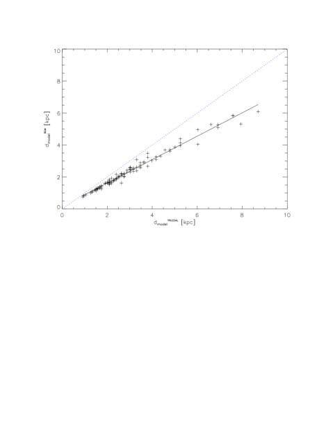
Figure 5: Comparison of model distances $d_{model}$ obtained from the Besançon Galaxy Model and the TRILEGAL model. The crosses indicate our calibration clusters from CCS 1. All distances are estimated for the A-sample of stars, a nearest neighbour number in the photometric decontamination of $N=25$ and a radius of $1\times r_{cor}$. We overplot a blue dotted one-to-one line as well as a black solid linear fit to the data.

We investigate if this calibration indeed removes the apparent dependence of our calculated distances on the specific galactic model used. For this purpose we compared the distances obtained from the Besançon Galaxy Model (Robin et al., 2003) with values estimated by using the TRILEGAL model from (Girardi et al., 2012, 2005). Distances from the latter model are obtained in the same way as described in Sect. 2.4 for the BGM. In Fig. 5 we show one example of a comparison of the two model distances $d_{model}$ obtained for the CCS 1 sample of clusters. The two distances depend linearly on each other, i.e. the TRILEGAL model predicts distances which are a factor of about 1.3 times larger than the distance from the BGM. However, since this is a linear relationship, our calibration described above will entirely remove this difference. If we would use the TRILEGAL model our calibration would simply result in a slightly different value for the parameter $C_{1}$ in Eq. 10. This shows that our calibration procedure removes any systematic dependence on the specific galactic model used, since every other model will behave in a similar way. Thus, our distances are model independent. We further note that the scatter in Fig. 5 is only 5.5 %, i.e. much smaller than the final uncertainty of our distances (see Sect. 2.6). Hence the contribution of the galactic model to the statistical noise of our method is negligable.

2.6 Optimisation of Distance Determination

The above described corrections and calibrations are performed for each combination of the ’free’ model parameters. Hence, we repeat the calibration procedure for the A-sample and C-sample of stars, the two sets of CCSs, cluster areas from one to three core radii and the nearest neighbour number (during the membership probability calculations) from 10 to 30.

For each set of free parameters we determine the scatter $S_{cal}$ to identify the parameter set that leads to the best calibration, i.e. the lowest scatter. Here we briefly discuss the results and implications of this optimisation exercise.

• Photometric Samples: For CSS 1 there is a noticeable overall lower value for the scatter $S_{cal}$ for the A-sample compared to the C-sample, the actual size of which depends on the other parameters. However, for CSS 2 there is no significant change in the scatter $S_{cal}$ between the A-sample and the C-sample, independent of other parameter values. As the aim of our project is to find a method of distance determination for a homogeneous data set of clusters, we choose the A-sample for our calibration and the final distance calculations.

• Photometric Decontamination: The nearest neighbour number $N$ used in the determination of the membership probabilities generates no trends or significant differences in the scatter $S_{cal}$ for CSS 1 and CSS 2. In other words, if we only vary $N$ and keep all other parameters the same, the scatter $S_{cal}$ randomly fluctuates by a few percent, much less than the variations caused by changes in one of the other parameters. This shows that the decontamination procedure is independent of this parameter value (in the investigated range of $10\leq N\leq 30$) for our calibration samples. This is understandable since $N$ only determines the resolution with which we can identify potential cluster members in CCM space (as discussed in Sect. 2.2) and has no influence on the colours of the most likely members which is used to determine the distances. To avoid any random fluctuations due to the choice of $N$ (even if small) we hence choose two values for this parameter ($N=15$ and $N=25$) for the distance calculations.

• Cluster Area: We vary the radius of the cluster area between one and three times $r_{cor}$. As for the choice of $N$, we find that there is no significant variation of the scatter $S_{cal}$ with cluster area. However, due to the nature of the star density profile (Sect. 2.1), the majority of cluster members will be within 1$\times r_{cor}$, most cluster members will be within 2$\times r_{cor}$, and the additional stars between 2 and 3$\times r_{cor}$ will be most likely field stars. Therefore, we only use 1$\times r_{cor}$ and 2$\times r_{cor}$ in the calibration and final distance calculation.

• Cluster Calibration Samples: We spilt CCS 2 into ’old’ (Log(Age[yrs]) $\geq 8.5$) and ’young’ (Log(Age[yrs]) $<8.5$) subsets, CCS 2_o and CCS 2_y respectively. We then use these to investigate if/how the scatter $S_{cal}$ varies with the mean age of the calibration sample. We find that there is no statistically significant change in $S_{cal}$ produced by CCS 2 and CSS 2_o. However, the scatter produced by CSS 2_y randomly fluctuates depending on the other parameters. Additionally, there is an overall increase in the scatter when using CCS 2_y compared to the entire CCS 2 sample. This could be due to the fact that a younger cluster sample, such as CCS 2_y, will contain clusters which have a high fraction of YSOs with high K-band excess. These stars could result in an inaccurate determination of $HK_{med}$ (see below in Sect. 2.7), and thus an erroneous number of foreground stars which in turn can lead to a higher scatter in the calibration. Therefore, our calibration should be applied to either a sample with a range of ages or an older sample. We choose CCS 1, as it gives consistently a smaller scatter $S_{cal}$ compared to CCS 2. Based on the above discussion all determined distances for clusters with a large fraction of YSOs, should be treated with care.

In summary, we find that the A-sample of stars in conjunction with CCS 1 leads consistently to the smallest scatter for the distance calibration. We find no significant or systematic influence of the radius of the cluster area or the nearest neighbour in the photometric decontamination on the quality of our method.

We therefore choose four different sets of parameter values to determine the distance to all FSR candidate clusters. The parameter values and the corresponding scatter $S_{cal}$ for CCS 1 and CCS 2 are listed in Table 1. The final distance for each cluster (listed in Table LABEL:app_table in the Appendix) is then determined as the median of the four distances from these calibration sets utilising CCS 1. The typical scatter and hence the accuracy of our distance calculation is better than 40 %, considering the intrinsic scatter of 30 % for the distances of the calibration sample Froebrich et al. (2010).

Table 1: Scatter $S_{cal}$ [%] of the four selected calibration sets for CCS 1 and CCS 2. All calculations are done with the A-sample of stars. The final cluster distances are determined as the median of the four distances determined using the calibration for CCS 1. N lists the nearest neighbour number in the photometric decontamination and Radius the distance out to which stars are included into the cluster area.

	N	Radius	$S_{cal}$ (CCS 1)	$S_{cal}$ (CCS 2)
		[$r_{cor}$]	[%]	[%]
Set 1	15	1	36	54
Set 2	25	1	37	50
Set 3	15	2	40	55
Set 4	25	2	46	56

2.7 Identification of Young Stellar Objects

We aim to identify and determine the fraction of YSOs ($Y_{frac}$) in each cluster candidate. This is vital for the determination of the extinction values (see Sect. 2.8), since disk excess stars can potentially lead to an overestimate of the colour excess and thus the wrong extinction. Furthermore, clusters with a significant fraction of YSOs are young. Thus, $Y_{frac}$ is also an important age indicator for the cluster. For each cluster candidate, the $Y_{frac}$ calculation (as described here) is repeated for every calibration set as described in Sect. 2.6.

We identify YSOs in each cluster by calculating the reddening free parameter $Q$ for each star in the cluster area. We define $Q$ as:

$$Q=(J-H)-\frac{E(J-H)}{E(H-K)}\times(H-K)$$ (13)

Where $(J-H)$ and $(H-K)$ are the NIR colours of the star. We use a value of $E(J-H)/E(H-K)=1.55$ (Mathis, 1990) for all determinations of $Q$. We consider an object a disk-excess source (or YSO) if its $Q$ value is smaller than $-$ 0.05 mag by more than 1 $\sigma$ (estimated from the photometric uncertainties).

Similar to the $HK_{med}$ determination (Sect. 2.3), we calculate $Y_{frac}$ for the top 25 % to 45 % of the highest probability member stars, in 5 % increments i.e. five $Y_{frac}$ values are determined for each cluster and calibration set. The final value for $Y_{frac}$ listed in Table LABEL:app_table in the Appendix is the median of the individual YSO fractions averaged over the four calibration sets.

To determine the YSO fraction we count the potential YSOs in the cluster and the total number of cluster members, $N_{YSO}$ and $N_{cl}$ respectively :

$$N_{YSO}=\sum\limits^{N}_{i,Q\leq-0.05mag}P^{i}_{cl}$$ (14)

$$N_{cl}=\sum\limits^{N}_{i}P^{i}_{cl}$$ (15)

Where $N_{YSO}$ is the number of potential YSOs that are members of the cluster, $N_{cl}$ is the number of all cluster members and $N$ is the number stars in the top 25 % to 45 % of the highest probability cluster members.

The YSO fraction is in principle the ratio of $N_{YSO}$ and $N_{cl}$. However, the number of YSOs is typically small and potentially influenced by photometric scatter. We thus determine a limit for the YSO fraction by assuming that each cluster contains at least $N_{YSO}-\sqrt{N_{YSO}}$ young stars:

$$Y_{frac}=\frac{N_{YSO}-\sqrt{N_{YSO}}}{N_{cl}}$$ (16)

If $Y_{frac}$ is a negative value, i.e. there are less than one YSOs in the cluster, the YSO fraction is set to zero.

2.8 Extinction Calculation

In addition to distance, we aim to determine the extinction to all FSR cluster candidates using the colour excess of the most likely cluster members we identified in Sect. 2.2. As for the determination of the fraction of YSOs in the cluster (Sect. 2.7), the extinction calculation (as described here) is repeated for every calibration set as described in Sect. 2.6. The final extinction value for each cluster candidate as quoted in Table LABEL:app_table in the Appendix is the median of the four individual extinction values.

For our calculation we utilise two different colours:

i) ($H-K$), which we used in Sect. 2.3 to identify foreground stars; The ($H-K$) colour is less well suited to determine the extinction, since its intrinsic value for stars depends on the spectral type as well as the luminosity class of the object. Generally this colour can range from 0.0 mag for A-stars to 0.4 mag for the latest spectral types (excluding rare OB stars and L-type brown dwarfs). More typical average colours for our observed clusters are between 0.1 and 0.3 mag. The advantage of the ($H-K$) colour is that we can determine it for every star in the cluster area.

ii) ($H-[4.5]$), which we estimate from the combination of WISE and 2MASS; The intrinsic ($H-[4.5]$) colour is almost independent of spectral type and luminosity class (Majewski et al., 2011) since it measures the slope of the spectral energy distribution in the Rayleigh-Jeans part of the spectrum. Hence, it has a well defined zero point. However, due to the lower resolution and depth of WISE, we can determine this colour only for about half the stars in the cluster area.

Since both utilised colours use the H-band, this is the natural pass band we determine the extinction in.

We calculate the H-band extinction $A_{H}^{H45}$ from the ($H-[4.5]$) colour excess by means of:

$$A_{H}^{H45}=\frac{A_{H}}{A_{H}-A_{4.5}}\times\left<H-[4.5]\right>$$ (17)

Where $\left<H-[4.5]\right>$ denotes the colour excess between the observed $(H-[4.5])$ colour and the zero point. We utilise the zero point of ($H-[4.5]$)${}_{0}=0.03$ mag valid for main sequence stars (Majewski et al., 2011) and the extinction law $A_{4.5}/A_{H}=0.28$ from (Indebetouw et al., 2005).

We calculate the H-band extinction $A_{H}^{HK}$ from the ($H-K$) colour excess using:

$$A_{H}^{HK}=\frac{A_{H}}{A_{H}-A_{K}}\times\left<H-K\right>$$ (18)

Where $\left<H-K\right>$ denotes the colour excess between the observed ($H-K$) colour (identical to $HK_{med}$, see Sect. 2.3) and the zero point. We again utilise the extinction law from Indebetouw et al. (2005) which gives $A_{K}/A_{H}=0.65$. To establish the zero point ($H-K$)₀ we plot $A_{H}^{H45}$ against $HK_{med}$ for all clusters with $A_{H}^{H45}<$ 1 mag and determined the off-set. We find that ($H-K$)${}_{0}=0.06$ mag.

This method will naturally overestimate the extinction for clusters with an enlarged population of YSOs and hence disk excess emission stars. The excess colour in these cases is caused by warm dust in the disk and not foreground extinction. We identify clusters for which this may be an issue via the fraction of intrinsically red sources in the NIR colour-colour diagrams (see Sect. 2.7). We consider all clusters with $Y_{frac}$ above 10 % as YSO clusters. These objects are excluded from the statistical analysis in this paper, but note that the fraction of such clusters in the FSR sample is rather low (see Sect 3.2).

3 Results

Our calibration and optimisation procedure requires that for each cluster there are at least 30 stars in the A-sample within one cluster core radius and that the core radius is smaller than 0.05^∘ (Sect 2.2). We further exclude all known globular clusters and clusters where the distances from the four calibration sets (see Sect. 2.6) scatter by more than 3 $\sigma$ compared to the average cluster. These requirements result in 1017 FSR objects being excluded, of which 931 are open clusters or candidates.

We determine the distance to 771 of the FSR objects i.e. 43 % of the entire FSR sample, of which 377 are known open clusters and 394 are new cluster candidates. Based on the total numbers of these objects in the FSR list (681 known clusters and 1021 new cluster candidates), these are 55 % and 39 %, respectively. This reflects the fact that in comparison to the new FSR cluster candidates, the known clusters should have, on average, more members and hence will more likely pass our selection criteria. The new FSR cluster candidates are typically less pronounced and a fraction of about 50 % of them might not be a real cluster (Froebrich et al., 2007). This has also been confirmed by the analysis of spatially selected sub-samples of the FSR cluster candidates by Bica et al. (2008) and Camargo et al. (2010). They find that about half the investigated candidates are star clusters with a tendency that overdensities with less members are more likely not real clusters. We finally note that the current version of the open cluster database from Dias et al. (2002) contains at the time of writing 141 of the 1022 FSR cluster candidates which have been followed up by the community. Hence, even without a complete and systematic analysis of the entire sample, 15 % of the clusters have already been identified as real objects. All of this evidence indicates that at least three quarters of all the confirmed clusters and cluster candidates investigated here are real, or that the contamination of our cluster sample is less than 25 %.

Further to the distances, we calculated the extinction and YSO fraction for 775 cluster candidates (43 % of the FSR sample, excluding globular clusters). The split of this group into known clusters and new candidates is 378 and 397 objects, respectively, or 56 % and 39 % of the entire cluster sample. In the following we will analyse the statistical properties of the entire sample. We will not aim to gauge which of the individual cluster candidates is real or not. This will be done in a forthcomming paper after the ages of the candidates have been determined. However, to aid the reader in evaluating the trustworthyness of individual properties we add two columns to Table LABEL:app_table in the Appendix. We list as $N^{tot}_{2r_{core}}$ the number of stars in the A-sample within two core radii for each cluster. We furthermore sum up all membership probabilities ($P^{i}_{cl}$) of these stars to determine the total estimated number of cluster members $N^{mem}_{2r_{core}}$ in the same area. As a guide we note that the contrast, i.e. the ratio of cluster members to field stars, is on average twice as high for the known clusters than for the new candidates. This is a clear indication that more pronounced objects are more likley to be real clusters.

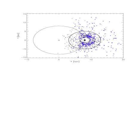
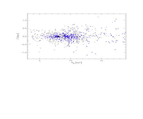
Figure 6: Left: Plot of the distribution of FSR clusters in the Galactic Plane based on the distances determined in this paper. The Galactic Centre is represented by a triangle. The smaller of the three circles indicates a distance of 1.5 kpc from the Sun, the medium sized circle indicates a distance of 5 kpc from the Sun, and large circle indicates a distance of 8 kpc from the Galactic Centre. Right: Plot of the height, Z, above and below the Galactic Plane of our clusters as a function of the Galactocentric distance, $R_{gc}$. In both plots black crosses represent new cluster candidates, blue stars represent previously known open clusters and the Sun is represented by a black square.

3.1 Cluster distribution in the Galactic Plane

We investigate how the clusters with distances are distributed in the Galactic Plane (GP) and determine completeness limits and selection effects. In Fig. 6 we show the positions of all clusters projected into the GP and the position with respect to the GP as a function of the Galactocentric distance. Note that for all these plots we assume a distance of 8 kpc of the Sun to the Galactic Centre.

The density of clusters per unit area in the GP for our sample peaks at about 3 kpc distance from the Sun. We find that averaged over the entire longitude range there are about 15 star clusters per square kiloparsec projected into the GP at a distance of 3 kpc from the Sun in our sample. At 4 kpc distance the density drops to about half this level. Also towards smaller distances, a similar significant drop in the density of clusters is found. The latter is caused by the well known selection effect in the FSR list, which includes only clusters of a certain apparent radius Froebrich et al. (2010). Thus, many nearby clusters were not included in the original FSR sample, or have been excluded by our condition that the cluster core radius should be smaller than 0.05^∘ (see Sect. 2.5.1). The drop in numbers at larger distances is in part caused by the same effect – the clusters are too compact to be included – and more distant objects are also too faint.

The scale height of the clusters with respect to the GP has been calculated for various sub-samples of our clusters. We excluded all clusters that have a distance of more than 5 kpc, since we are more likely to detect clusters further away from the mid-plane at large distances due to extinction. The known clusters in our sample have a scale-height of 235 $\pm$ 20 pc while the new cluster candidates have a distribution with a width of 315 $\pm$ 30 pc. We also split our sample in potentially younger and older clusters via the fraction of YSOs (old: $Y_{frac}<$ 1 %; young $Y_{frac}>$ 1 %). Then we find for the young clusters a scale-height of 190 $\pm$ 15 pc, and for the older clusters 300 $\pm$ 20 pc. These scale heights are in between the numbers for clusters older and younger than 1 Gyr in the FSR sample (older: 375 pc; younger 115 pc; Froebrich et al. (2010)). It is also larger than the scale height of the dust in the solar neighbourhood (125 pc (Drimmel et al., 2003; Marshall et al., 2006)). The potentially younger clusters in our sample show a higher degree of concentration to the GP. In Paper II we will determine the ages of all clusters and candidates to investigate in more detail the age dependence of the scale height.

As can be seen in the original FSR paper (Froebrich et al., 2007) and also amongst the old FSR clusters (Froebrich et al., 2010), the distribution of the clusters along the GP is not homogeneous. In particular towards the GC the sample is incomplete. This is most likely caused by crowding and low contrast between cluster and field stars. For the older clusters, some of this could be a real effect since old open clusters seem to exist in lower numbers at Galactocentric distances smaller than that of the Sun (Friel, 1995).

Here we utilise Kolmogorov-Smirnov tests (see e.g. Peacock (1983)) to investigate if subsamples of the FSR clusters have similar distributions or if they are different. We compare five different samples:

• Clusters with $Y_{frac}<5$ %; old clusters

• Clusters with 5 % $<Y_{frac}$; young clusters

• Known open clusters amongst the FSR sample

• New FSR cluster candidates

• All FSR clusters, except known globulars

We determine the probability that any two of the samples are randomly drawn from the same parent distribution. We also test the clusters in each sample against a homogeneous distribution (SH). For this we only use clusters that are more than 60^∘ away from the GC, since we know that close to the GC the FSR list is incomplete (Froebrich et al., 2007). We summarise the results in Table 2.

These tests do reveal that most of the samples have a different distribution along the GP. In particular, the sample of potentially old clusters (S1) seems to be different from most of the other sub-samples. Note that probabilities larger than 1 % and less than 99 % in the KS-test are not significant.

Table 2: KS-test probabilities that two of our cluster sub-samples are drawn from the same parent distribution. S1: older clusters, $Y_{frac}<5$ %; S2: young clusters, 5 % $<Y_{frac}$; S3: Known FSR clusters; S4: New cluster candidates; S5: All FSR clusters, except known globular clusters; SH: A homogeneous distribution along the GP – but more than 60^∘ away from the GC.

	S1	S2	S3	S4	S5	SH
S1	—	0.25	0.02	2.53	0.43	33.8
S2	0.25	—	39.5	4.07	9.89	17.2
S3	0.02	39.5	—	0.51	15.4	52.2
S4	2.53	4.07	0.51	—	44.6	69.6
S5	0.43	9.89	15.4	44.6	—	76.0
SH	33.8	17.2	52.2	69.6	76.0	—

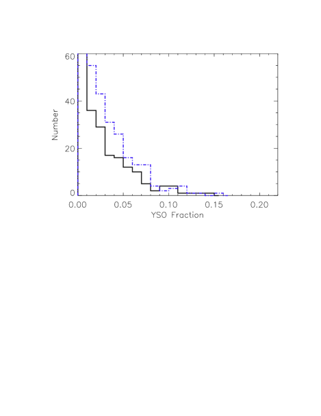
Figure 7: Histogram showing the distribution of $Y_{frac}$ of our sample. The solid black line represents new cluster candidates and the dot-dash blue line the known open clusters. The peak in the first bin ($Y_{frac}<$ 1 %) is too high to be shown – 258 new cluster candidates and 165 known open clusters.

3.2 Young Clusters

In Paper II we will determine the ages of all our cluster candidates and investigate the age distribution as well as how the cluster properties such as scale height change with age (as discussed above in Sect. 3.1). So far the only measure of age we have is the fraction of young stars ($Y_{frac}$) in each cluster as determined in Sect. 2.7. In Fig. 7 we show the distribution of the YSO fraction for all clusters.

There is a steep decrease of the number of clusters with increasing YSO fraction and only a small number of cluster candidates have a high $Y_{frac}$. The sample is dominated by clusters with essentially zero YSOs. Only 18 cluster candidates have $Y_{frac}>$ 10 %, and no objects have $Y_{frac}>$ 20 %. The apparent lack of clusters with $Y_{frac}>$ 20 % in our sample means there are potentially no clusters with an age of less than 4 Myrs – according the relation of YSO fraction and age for embedded clusters from Lada & Lada (2003). There are two obvious reasons for this: i) the FSR list is assembled from NIR 2MASS overdensities, hence will naturally lack young and embedded objects. ii) We do not include L-band excess stars in our YSO fraction, and our YSO fraction is a lower limit. Using the L-band would require us to include the WISE photometry, and we have seen in Sect. 2.8 that only about half the 2MASS sources in each cluster can be reliably cross-matched to their WISE counterparts.

The four clusters with the highest YSO fraction are FSR 0488 (Teutsch 168), FSR 1127 (NGC 2311), FSR 1336 (a new cluster candidate) and FSR 1497 (Ruprecht 77).

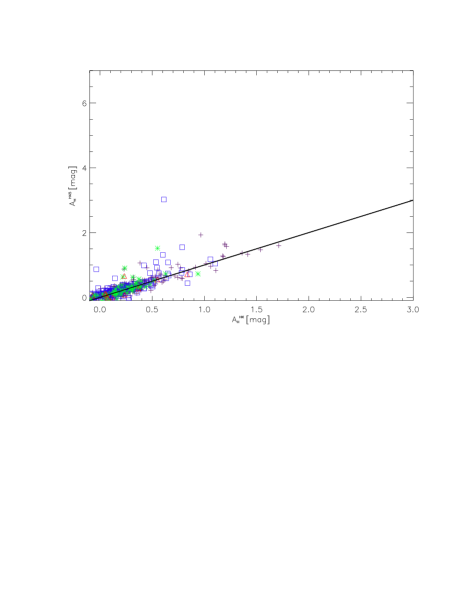
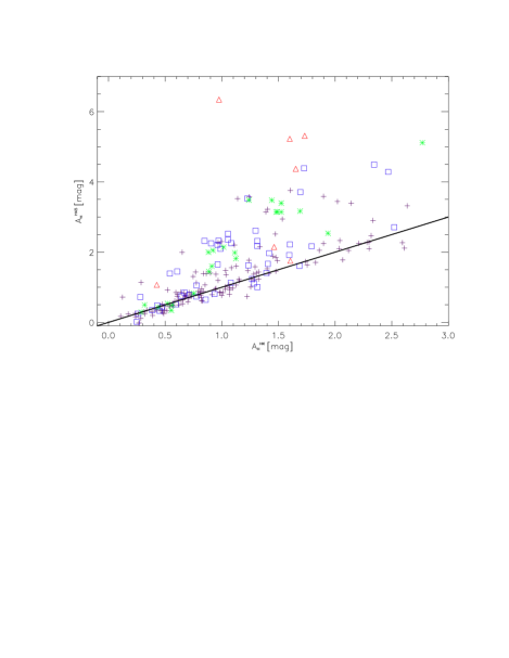
Figure 8: Plot of $A_{H}^{HK}$ against $A_{H}^{H45}$. Red triangles represent clusters with $Y_{frac}>0.10$, green stars are clusters with $0.05<Y_{frac}<0.10$, blue squares are clusters with $0.01<Y_{frac}<0.05$ and purple crosses are clusters with $Y_{frac}<0.01$. The left panel includes all clusters with distances $d_{cal}<5$ kpc and the right panel all clusters more distant than 5 kpc or where we did not estimate a distance but the extinction.

3.3 Extinction Law

As outlined in Sect. 2.8, we determine a zero point of $(H-K)_{0}$ = 0.06 mag by comparing the cluster extinction values determined from $(H-K)$ and $(H-[4.5])$ colour excess and excluding clusters with $Y_{frac}>0.10$. In Fig. 8 we show how the H-band extinction values calculated from the two colour excesses compare to each other. The vast majority of clusters follow the one-to-one line with a $rms$ of 0.18 mag in $A_{H}$. This even holds for clusters where we were unable to determine a reliable distance.

There are a number of clusters for which the extinction calculated from the $(H-[4.5])$ excess is significantly higher than that calculated from the $(H-K)$ excess. These differences are most likely due to the fact that only the brightest $[4.5]$ $\mu$m sources are matched to 2MASS and hence the extinction calculation is biased towards intrinsically redder objects. We exclude all clusters more than 3 $\sigma$ above the one-to-one trend line from our subsequent analysis of the dependence of the extinction on the cluster distance.

We estimate how the extinction per unit distance changes for our cluster sample as a function of Galactic longitude. To establish a reliable value, we apply the following restrictions to our cluster sample: i) All clusters have to be closer than 5 kpc to the Sun in order to ensure a reliable distance; ii) The fraction of YSOs should be smaller than 10 % for the extinction not to be influenced by disk excess emission stars; iii) Clusters have to be closer than 150 pc to the GP to ensure the line of sight is mostly in the Galactic midplane; iv) The extinction of the cluster determined from $(H-[4.5])$ and $(H-K)$ excess differ by less than 3 $\sigma$ compared to the one-to-one trend line.

In the left panel of Fig. 9 we show an example of how $A_{H}^{HK}$ depends on the distance for our clusters. Only clusters at $l=110\pm 30^{\circ}$ are shown. The overplotted solid line is the best linear fit, boxed crosses indicate the clusters used, whilst un-boxed crosses mark the clusters excluded by a 3 $\sigma$ clipping. The fit indicates an extinction law of 0.17 mag/kpc extinction in the H-band. Converted to optical extinction using Mathis (1990) this is $A_{V}$ = 0.9 mag/kpc.

We investigate how this extinction law changes as a function of Galactic longitude in the right panel of Fig. 9. We determine the extinction per unit distance every 10^∘ of Galactic longitude, but include all clusters that are within 30^∘. We find that there is a systematic dependence of the extinction per unit distance. The lowest values ($A_{H}=$ 0.1 mag/kpc) are found near the Galactic Anticentre and a steady increase is observed towards the GC where almost $A_{H}=$ 0.3 mag/kpc is reached. We only determined the extinction law if there are at least 10 clusters available in the longitude bin. It is important to note, that in regions closer than 60^∘ to the GC, very few clusters are available. Figure 9 also shows that the general behaviour of the extinction values is similar for both $A_{H}^{HK}$ and $A_{H}^{H45}$; they are mostly indistinguishable within the uncertainties.

The canonical value of the extinction per unit distance, $A_{V}=$ 0.7 mag/kpc (e.g. Froebrich et al. (2010)), converts to $A_{H}=$ 0.12 mag/kpc. This is in agreement with our estimates for large regions towards the Galactic Anticentre, but does not hold for lines of sight closer towards the GC. There, values at least two or three times the canonical value seem to be more appropriate. We find that the longitude dependence of the extinction can best be described as:

$$A_{H}(l){\rm[mag/kpc]}=0.1+0.001\times\left|l-180^{\circ}\right|/^{\circ},$$ (19)

for lines of sight of more than $60^{\circ}$ from the Galactic Centre. Our calibration with respect to the Galactic longitude (see Sect. 2.5.4) is thus only needed because we used a constant $A_{V}$/kpc in the BGM. If one employs our position dependent value for the ISM extinction in the model, then only the crowding and extinction corrections (Sect. 2.5.3) are required. In principle this could ensure the usability of our method without a calibration sample.

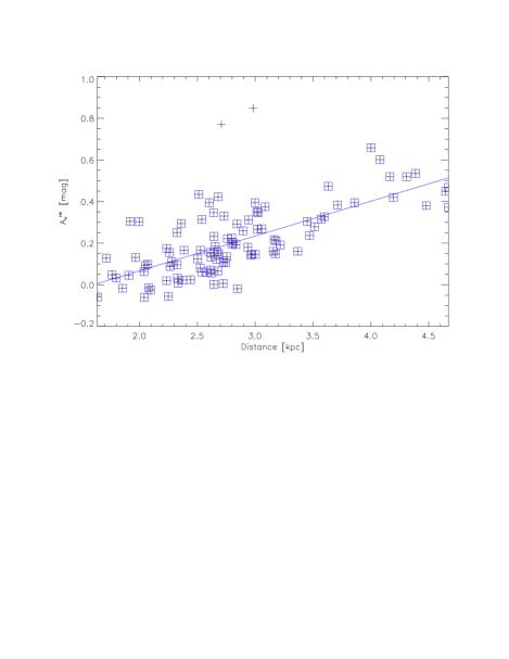
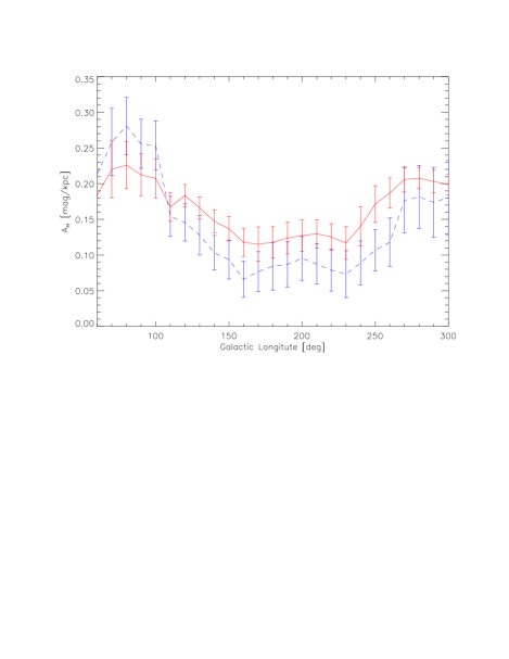
Figure 9: Left: The plot shows $A_{H}^{HK}$ against our calibrated distance values for clusters with $l=110^{\circ}\pm 30^{\circ}$. Crosses represent clusters in this region, and boxed crosses are clusters which were not excluded from the fit by our $3\sigma$ clipping. Right: This shows the H-band extinction per unit distance as a function of Galactic longitude. The red solid line represents $A_{H}^{HK}$ per kpc and the blue dashed line $A_{H}^{H45}$ per kpc.

3.4 Potential Improvements

One consequence of using 2MASS data to identify stars foreground to the clusters is that the data has a resolution of about $2"$ (Skrutskie et al., 2006). Thus, we are unable to resolve close (apparent) binaries and to detect faint cluster members. In other words, crowding in dense cluster centres and generally near the GC or the Galactic Plane is the limiting factor in our accuracy.

With the availability of deeper homogeneous photometry data sets, such as UKIDSS-GPS (Lucas et al., 2008) and VISTA-VVV (Minniti et al., 2010) better NIR data will be available for studies of large samples of clusters (e.g. Chené et al. (2012)). These deeper and higher resolution data will not only allow the detection of fainter cluster members, it also allows a more accurate determination of the density of stars foreground to the cluster, since deeper observations generally detect more foreground dwarfs than background giants. Furthermore, these data will also allow us to study more compact and distant clusters, which are currently excluded due to the low spatial resolution.

4 Conclusions

We present an automatic calibration and optimisation method to estimate distances and extinction to star clusters from NIR photometry alone, without the use of isochrone fitting. We employed the star cluster decontamination procedure from Bonatto & Bica (2007b) and Froebrich et al. (2010) to calculate the number of stars foreground to clusters and the Besançon Galaxy Model (Robin et al., 2003) to estimate uncalibrated model distances.

Our method has been calibrated using two calibration sets of known open clusters. We utilise a homogeneous list of 206 old ($>$100 Myr) open clusters from the FSR list (Froebrich et al., 2010) as well as all WEBDA entries amongst the FSR clusters. Due to the nature of the entries in the WEBDA database the latter calibration set is inhomogeneous, but covers a larger range of ages. We find that the older FSR clusters provide the best calibration sample and we achieve a distance uncertainty of less than 40 % after the calibration. Our calibration procedure ensures that all our results are independent of the specific galactic model used.

Using our calibration method, we determined the distances to 771 cluster candidates from the FSR list. Of these, 377 were known open clusters and 394 are new cluster candidates. We also determine the extinction to 775 clusters, 378 known and 397 new candidates. Based on the Q-parameter we also estimate the YSO fraction for each cluster in our sample.

The spatial density of clusters per unit area in the GP for our sample peaks at about 3 kpc distance from the Sun. Thus, our sample is biased towards clusters of this distance and lacks more distant and closer objects. This is caused by the well known selection effect in the FSR list, which includes only clusters of a similar apparent radius (Froebrich et al., 2010). The scale height of the younger clusters (YSO fraction above 1 %) is 190 pc, while the remaining (older) clusters show a scale height of 300 pc.

We investigated how the extinction per unit distance to the clusters changes as a function of Galactic longitude. There is a systematic dependence that can at best be described by $A_{H}(l)$ [mag/kpc] = 0.1 + 0.001$\times\left|l-180^{\circ}\right|/^{\circ}$ as long as the clusters are more than 60^∘ from the GC and not embedded in Giant molecular clouds. We suggest use of this extinction law, instead of a constant canonical value for any simulations performed with the Besançon Galaxy Model. In turn this allows to use our procedure for distance estimates without the need for a calibration sample. In particular, for clusters in the GP but not projected onto Giant Molecular Clouds, the $\left<H-[4.5]\right>$ colour excess can be used as a distance indicator – at least statistically.

Appendix A FSR Cluster Property Table

Table 3: Summary table of the FSR cluster properties determined with our method. The table lists the FSR ID number, the cluster type (known open cluster or new cluster candidate), the Galactic coordinates and RA and DEC (J2000), the distance in kiloparsec, the $H$-band extinction values calculated from $H-K$ excess ($A_{H}^{HK}$) and from $H-[4.5]$ excess ($A_{H}^{H45}$), the YSO fraction ($Y_{frac}$), the number of stars within two core radii of the cluster centre ($N^{tot}_{2r_{core}}$), and the total number of members (calculated as the sum of the membership probabilities of all stars) in the same area ($N^{mem}_{2r_{core}}$).

FSR	Type	l	b	RA	DEC	d	$A_{H}^{H45}$	$A_{H}^{HK}$	$Y_{frac}$	$N^{tot}_{2r_{core}}$	$N^{mem}_{2r_{core}}$
ID		[deg]	[deg]	(J2000)	(J2000)	[kpc]	[mag]	[mag]
0001	new	0.03	03.47	17:32:22.2	-27:03:41	4.4	0.91	1.06	0.00	1015	342
0002	new	0.05	03.44	17:32:32.4	-27:03:52	4.3	0.84	1.05	0.00	365	111
0009	new	1.86	-09.52	18:28:29.9	-31:53:49	3.4	0.05	0.32	0.00	286	73
0018	new	5.34	05.41	17:37:41.4	-21:33:27	4.1	0.41	0.53	0.00	1333	337
0019	new	5.52	06.08	17:35:39.3	-21:02:50	3.8	0.27	0.44	0.00	654	233
0022	new	6.18	00.84	17:56:28.8	-23:11:36	6.3	1.01	0.99	0.00	456	237
0023	new	6.58	00.78	17:57:35.1	-22:52:34	-	0.81	1.28	0.00	139	34
0025	new	7.54	05.65	17:41:43.6	-19:34:14	3.6	0.40	0.52	0.00	419	118
0027	new	7.78	08.45	17:32:12.8	-17:53:03	2.6	0.12	0.34	0.00	132	35
0031	new	8.91	-00.27	18:06:29.0	-21:22:34	4.1	2.17	2.35	0.00	1121	354
0032	known	9.28	-02.53	18:15:48.2	-22:08:22	2.8	0.40	0.21	0.00	239	83
0035	new	9.69	00.76	18:04:16.5	-20:11:26	-	2.40	2.09	0.00	650	168
0039	new	10.25	00.32	18:07:05.3	-19:54:59	4.3	1.85	2.12	0.00	336	109
0042	new	11.79	16.13	17:14:05.7	-10:28:21	0.7	0.31	0.25	0.00	199	62
0045	known	12.87	-01.32	18:18:29.9	-18:24:12	2.2	0.66	0.20	0.02	265	127
0047	known	14.04	-00.82	18:18:59.6	-17:08:02	6.1	2.34	2.65	0.00	330	125
0050	new	16.39	11.41	17:39:51.6	-09:06:04	1.0	0.32	0.44	0.01	184	55
0051	new	16.71	02.24	18:13:04.6	-13:19:51	4.0	1.00	1.12	0.00	544	147
0052	new	16.79	-02.92	18:32:04.0	-15:41:19	5.6	0.65	0.75	0.00	1165	266
0053	known	16.97	00.83	18:18:40.7	-13:46:43	3.0	0.51	0.89	0.03	370	188
0054	new	17.16	-02.28	18:30:24.4	-15:03:49	3.6	0.05	0.32	0.00	134	54
0055	new	17.99	-00.28	18:24:42.1	-13:23:41	6.8	2.36	2.35	0.00	266	97
0057	known	18.46	-00.40	18:26:03.5	-13:02:06	4.8	1.95	1.51	0.00	567	205
0059	new	19.74	-00.56	18:29:04.1	-11:58:29	6.8	2.18	2.67	0.00	108	30
0060	new	20.29	-00.56	18:30:05.8	-11:29:09	7.3	2.35	2.33	0.00	1369	373
0062	new	20.86	04.30	18:13:46.0	-08:42:30	2.0	0.28	0.54	0.00	312	117
0063	new	21.26	04.14	18:15:05.1	-08:26:10	5.4	0.86	0.97	0.00	238	58
0068	known	22.85	-00.63	18:35:11.0	-09:15:07	-	2.32	2.26	0.00	1119	376
0070	new	23.44	-15.27	19:30:02.5	-15:10:04	3.6	0.99	0.57	0.00	95	31
0071	known	23.89	-02.91	18:45:19.0	-09:22:23	1.9	0.18	0.21	0.01	951	299
0072	new	24.70	00.31	18:35:12.7	-07:10:52	5.3	1.77	1.88	0.01	1182	307
0074	known	25.36	-04.31	18:53:03.4	-08:41:53	3.5	0.79	0.18	0.00	332	188
0076	new	25.56	05.08	18:19:50.3	-04:12:36	1.9	0.46	0.47	0.00	480	177
0077	new	25.71	05.05	18:20:13.9	-04:05:10	1.8	0.33	0.44	0.00	605	171
0080	new	26.64	12.19	17:56:38.4	00:03:28	1.1	0.10	0.26	0.00	85	35
0082	known	27.31	-02.77	18:51:04.3	-06:15:37	1.1	0.18	0.09	0.01	1007	498
0087	new	29.09	-00.44	18:46:00.0	-03:37:14	-	2.54	2.37	0.01	1302	420
0089	new	29.49	-00.98	18:48:39.2	-03:30:35	4.5	1.92	1.53	0.00	275	120
0090	new	29.62	-01.39	18:50:20.2	-03:34:42	6.2	1.18	1.34	0.02	398	164
0094	new	31.82	-00.12	18:49:50.7	-01:02:54	6.0	1.80	1.79	0.00	1550	569
0098	new	33.03	01.15	18:47:31.1	00:36:50	5.1	1.55	1.09	0.00	194	88
0100	new	34.33	-02.79	19:03:54.9	-00:01:36	3.4	0.30	0.32	0.00	307	107
0101	new	35.15	01.75	18:49:14.9	02:46:06	3.2	1.11	1.07	0.00	1099	355
0107	new	36.31	-03.21	19:09:02.9	01:32:11	5.0	0.35	0.53	0.00	489	137
0109	known	37.17	02.62	18:49:47.8	04:57:46	1.7	0.60	0.52	0.00	922	441
0111	known	38.66	-01.64	19:07:44.1	04:20:30	2.0	0.36	0.19	0.00	298	124
0112	new	38.68	-18.70	20:08:20.3	-03:32:18	1.2	0.15	0.17	0.00	98	37
0113	known	39.10	-01.68	19:08:42.2	04:43:10	1.6	0.46	0.29	0.00	659	239
0115	known	40.35	-00.70	19:07:32.1	06:16:21	2.4	1.09	0.80	0.01	237	85
0122	known	45.70	-00.12	19:15:28.6	11:17:13	2.1	0.76	0.64	0.01	425	218
0124	new	46.48	02.65	19:06:52.8	13:15:22	3.7	0.60	0.48	0.00	260	102
0126	new	48.55	-00.18	19:21:09.0	13:46:30	6.2	1.52	1.53	0.00	260	108
0127	known	48.89	-00.94	19:24:33.3	13:42:59	2.6	0.62	0.60	0.11	166	61
0129	new	49.39	-01.32	19:26:56.7	13:58:57	7.0	1.07	1.37	0.01	483	144
0133	new	51.12	-01.17	19:29:47.1	15:34:27	4.2	1.03	0.87	0.00	1227	637
0138	known	53.22	03.34	19:17:15.3	19:32:57	2.5	0.48	0.36	0.00	998	299
0142	new	55.79	-00.19	19:35:39.8	20:07:45	7.0	1.28	1.34	0.00	632	190
0143	new	56.32	-04.38	19:52:11.1	18:30:11	3.6	0.20	0.28	0.01	264	48
0144	known	56.34	-04.69	19:53:21.5	18:22:17	1.9	0.06	0.02	0.00	268	46
0148	new	57.03	00.02	19:37:28.8	21:18:54	2.8	0.92	0.61	0.00	120	55
0153	known	59.40	-00.15	19:43:10.0	23:17:49	4.1	0.52	0.60	0.00	123	69
0154	new	60.00	-01.08	19:47:58.4	23:21:03	3.2	0.49	0.54	0.02	653	234
0157	new	62.02	-00.70	19:51:03.5	25:17:05	2.2	0.48	0.58	0.00	389	152
0160	new	62.71	01.34	19:44:44.5	26:54:38	7.8	0.69	0.87	0.00	112	50
0161	new	63.10	-17.39	20:53:10.7	16:53:30	1.3	0.07	0.12	0.04	133	49
0162	new	63.21	-02.75	20:01:32.1	25:14:06	3.2	0.47	0.48	0.00	529	102
0163	new	63.23	-02.42	20:00:19.4	25:25:17	4.2	0.54	0.51	0.00	162	60
0165	new	64.10	-01.30	19:58:06.8	26:45:30	2.9	0.69	0.54	0.01	765	235
0166	new	64.87	-04.94	20:13:37.9	25:27:18	2.2	0.32	0.35	0.01	424	147
0167	new	65.16	-02.41	20:04:50.2	27:04:15	2.4	0.43	0.42	0.00	272	109
0168	known	65.53	-03.97	20:11:36.9	26:31:59	1.4	0.14	0.09	0.00	156	55
0169	known	65.69	01.18	19:52:13.2	29:23:59	2.5	0.16	0.08	0.01	275	111
0170	new	65.93	-02.69	20:07:46.2	27:33:55	6.7	1.62	1.14	0.00	214	75
0171	known	66.10	-00.94	20:01:28.5	28:38:50	3.7	0.81	0.70	0.02	250	89
0172	new	66.43	-00.36	20:00:01.3	29:13:30	4.8	0.84	0.87	0.00	647	201
0177	known	67.64	00.85	19:58:10.1	30:53:52	3.1	0.31	0.15	0.00	155	70
0180	known	68.01	02.87	19:50:58.9	32:15:18	8.2	0.42	0.48	0.00	168	48
0181	known	68.53	00.45	20:01:58.8	31:26:25	4.3	0.79	0.63	0.00	113	48
0182	new	69.18	03.36	19:51:46.8	33:30:44	2.7	0.13	0.07	0.00	397	136
0183	new	69.52	-09.54	20:42:13.3	26:35:17	2.8	0.11	0.28	0.00	120	46
0186	known	69.97	10.91	19:20:51.6	37:47:09	2.0	0.21	0.25	0.01	220	165
0187	known	70.31	01.76	20:01:10.0	33:38:41	4.5	1.21	0.34	0.00	513	126
0188	new	70.65	01.74	20:02:05.2	33:55:10	8.3	0.70	0.69	0.00	216	53
0189	new	70.66	-00.15	20:09:47.0	32:54:48	4.0	1.62	0.84	0.02	330	78
0190	new	70.73	00.96	20:05:28.4	33:34:30	10.2	1.31	1.31	0.00	229	83
0191	new	70.99	02.58	19:59:29.6	34:39:23	3.8	0.40	0.56	0.04	198	98
0192	new	71.10	00.85	20:06:52.0	33:49:49	8.6	0.68	0.88	0.00	270	110
0193	new	71.31	08.12	19:36:29.7	37:41:42	3.1	0.01	0.16	0.00	101	42
0194	known	71.87	02.42	20:02:25.4	35:19:15	9.5	1.46	0.92	0.00	191	72
0195	new	72.07	-00.99	20:16:51.6	33:37:38	4.1	0.79	0.99	0.06	253	124
0196	known	72.12	-00.51	20:15:03.1	33:56:10	2.9	0.46	0.44	0.04	410	154
0197	new	72.16	00.30	20:11:53.4	34:24:46	3.7	0.82	0.62	0.02	988	294
0198	new	72.18	02.62	20:02:24.9	35:41:21	12.8	1.72	1.02	0.03	275	117
0199	known	72.40	00.94	20:09:55.9	34:58:24	2.9	0.39	0.28	0.01	789	310
0200	known	73.25	00.95	20:12:10.5	35:41:06	3.8	0.41	0.34	0.01	1282	482
0201	known	73.27	01.17	20:11:18.1	35:49:24	5.3	0.36	0.36	0.00	806	291
0202	known	73.99	08.49	19:41:18.1	40:12:02	1.5	0.18	0.02	0.01	277	230
0204	new	74.78	00.61	20:17:46.0	36:45:60	8.1	2.33	1.14	0.04	225	63
0205	known	75.24	-00.67	20:24:21.3	36:25:01	6.9	1.59	1.45	0.00	151	89
0206	known	75.35	-00.49	20:23:55.2	36:36:24	3.8	0.91	0.84	0.01	304	85
0207	known	75.38	01.30	20:16:34.7	37:39:10	2.0	0.36	0.04	0.01	136	62
0208	known	75.70	00.99	20:18:47.7	37:44:19	3.2	0.41	0.42	0.02	602	289
0210	new	76.21	-00.55	20:26:37.5	37:16:54	6.6	1.44	1.33	0.00	259	100
0211	known	76.39	-00.60	20:27:22.7	37:23:41	7.5	2.97	2.39	0.00	115	11
0212	known	76.94	02.02	20:17:58.8	39:20:46	11.8	5.30	1.65	0.12	108	49
0213	new	77.63	00.38	20:26:59.3	38:58:34	5.7	1.20	1.13	0.03	617	216
0214	new	77.71	04.18	20:10:48.8	41:10:42	5.8	0.23	0.29	0.00	207	123
0216	known	78.01	-03.36	20:43:21.3	37:02:28	1.7	0.21	0.10	0.00	170	64
0218	known	78.10	02.79	20:18:04.6	40:44:22	2.7	0.57	0.37	0.01	419	168
0219	new	78.14	03.52	20:15:00.3	41:10:46	7.9	0.72	0.67	0.00	144	61
0220	known	78.15	-00.54	20:32:24.6	38:51:34	3.6	1.03	1.11	0.00	190	27
0224	new	78.47	01.36	20:25:21.7	40:13:39	5.5	2.07	0.70	0.00	266	98
0225	new	78.58	-02.80	20:42:53.2	37:49:45	4.0	0.54	0.65	0.01	189	80
0226	known	79.00	03.67	20:16:51.6	41:58:52	9.3	1.14	0.90	0.01	546	290
0230	known	79.31	01.31	20:28:10.3	40:52:54	10.3	3.51	2.07	0.00	180	38
0231	known	79.57	06.83	20:03:59.7	44:09:49	1.3	0.08	0.00	0.00	191	96
0233	known	79.87	-00.93	20:39:21.7	39:59:47	3.4	1.33	1.23	0.00	640	332
0234	known	80.13	00.75	20:33:06.1	41:13:10	5.6	1.04	1.15	0.00	911	386
0238	new	80.48	00.62	20:34:47.8	41:24:56	3.0	0.88	0.90	0.00	280	90
0239	new	80.52	02.94	20:24:46.8	42:49:05	11.2	1.46	1.47	0.00	284	101
0240	known	80.94	-00.17	20:39:37.3	41:18:39	9.0	3.39	2.69	0.00	95	38
0241	new	81.23	08.03	20:03:02.9	46:11:20	1.8	0.12	0.07	0.00	259	86
0243	known	81.46	01.11	20:35:48.8	42:29:45	5.4	1.25	1.21	0.00	116	53
0244	known	81.48	00.46	20:38:42.2	42:07:26	5.8	3.64	1.30	0.01	205	102
0245	new	81.50	00.62	20:38:05.8	42:13:54	6.5	2.04	1.47	0.01	132	75
0248	new	81.72	-00.60	20:43:57.6	41:39:27	7.6	2.12	1.91	0.00	265	88
0250	new	82.16	-16.99	21:44:58.6	30:44:56	1.6	0.10	0.10	0.00	113	42
0251	new	82.33	00.76	20:40:14.8	42:58:33	5.6	1.13	1.18	0.01	246	131
0254	new	82.81	05.79	20:18:51.5	46:18:32	3.9	0.24	0.37	0.00	183	42
0255	new	82.93	02.20	20:35:53.2	44:19:31	12.5	1.70	1.81	0.00	243	93
0256	known	83.08	-04.13	21:02:57.6	40:26:30	3.7	0.63	0.55	0.00	92	50
0257	new	83.13	04.84	20:24:24.0	46:02:24	2.8	0.16	0.26	0.03	248	121
0258	new	83.58	00.68	20:44:50.0	43:54:55	2.5	0.58	0.49	0.00	134	58
0261	new	83.99	-01.09	20:53:48.1	43:06:36	2.7	0.98	0.82	0.00	130	71
0262	known	84.89	03.80	20:35:15.9	46:51:26	7.7	0.82	0.73	0.00	406	138
0263	known	84.97	-00.22	20:53:34.8	44:25:13	5.4	1.54	1.28	0.00	505	125
0265	new	85.50	-04.44	21:12:50.0	42:00:34	2.5	0.34	0.37	0.01	326	80
0266	new	85.62	-16.15	21:54:06.3	33:35:02	1.6	0.06	0.12	0.00	125	32
0267	known	85.68	-01.52	21:01:42.7	44:06:54	2.0	0.44	0.36	0.06	151	48
0268	known	85.90	-04.14	21:13:08.6	42:30:22	3.6	0.54	0.43	0.00	218	182
0271	new	86.17	-05.28	21:18:35.8	41:55:10	3.0	0.31	0.33	0.00	291	93
0275	new	87.20	00.97	20:56:36.5	46:53:32	5.1	0.50	0.52	0.02	777	238
0276	new	87.32	05.75	20:34:29.5	49:57:21	7.4	0.55	0.62	0.00	242	74
0278	new	87.86	06.84	20:30:57.7	51:02:06	3.8	0.32	0.29	0.00	288	86
0280	known	88.24	00.26	21:03:47.0	47:12:37	4.5	0.52	0.43	0.00	568	166
0282	new	88.75	01.05	21:02:18.8	48:07:01	2.6	0.36	0.45	0.00	152	63
0284	new	89.07	02.60	20:56:28.6	49:22:08	2.7	0.25	0.18	0.03	283	108
0285	known	89.62	-00.39	21:12:09.7	47:46:54	2.4	0.18	0.22	0.05	273	113
0286	known	89.98	-02.73	21:23:29.4	46:24:18	1.8	0.16	0.09	0.00	166	84
0290	new	90.42	03.19	20:59:09.1	50:46:46	10.9	1.14	1.12	0.00	366	100
0293	new	91.03	-02.75	21:27:56.7	47:07:06	2.3	0.03	0.06	0.03	312	114
0294	new	91.27	02.34	21:06:44.9	50:51:25	2.7	0.35	0.48	0.02	180	91
0295	new	92.32	-00.16	21:22:39.0	49:52:38	2.9	0.44	0.36	0.00	167	50
0300	known	92.94	02.81	21:11:48.7	52:23:56	3.5	0.75	0.68	0.00	124	78
0301	known	93.04	01.80	21:16:58.8	51:46:10	4.0	0.75	0.71	0.02	182	116
0304	new	93.56	00.67	21:24:31.5	51:20:24	3.6	0.40	0.53	0.01	199	77
0308	known	94.40	-05.51	21:53:30.9	47:16:02	10.3	3.24	1.74	0.06	145	127
0309	known	94.42	00.19	21:30:38.1	51:35:07	1.7	0.26	0.18	0.01	767	277
0313	known	95.28	02.07	21:26:11.6	53:32:33	7.6	0.92	0.76	0.00	409	143
0316	new	96.07	-00.33	21:40:52.7	52:18:24	2.8	0.16	0.25	0.02	221	59
0318	new	96.15	-04.72	21:58:48.2	48:58:10	2.8	-0.04	0.20	0.02	145	42
0320	new	96.38	01.24	21:35:26.3	53:41:07	2.3	0.17	0.15	0.02	410	121
0322	new	96.47	-02.10	21:50:12.5	51:12:40	2.1	0.21	0.15	0.00	261	70
0324	new	96.54	01.26	21:36:09.5	53:48:55	2.5	0.29	0.18	0.03	620	191
0326	new	96.75	01.08	21:38:01.8	53:49:11	8.6	0.95	0.86	0.00	127	60
0327	known	97.34	00.45	21:43:51.8	53:43:29	3.1	0.51	0.43	0.04	397	105
0334	new	98.71	01.54	21:46:10.2	55:26:57	3.0	0.29	0.20	0.01	477	136
0336	new	99.09	00.96	21:50:51.8	55:14:49	2.5	0.38	0.37	0.02	709	231
0337	known	99.14	07.49	21:18:03.7	60:05:32	13.0	1.46	0.89	0.00	247	110
0340	known	99.31	03.74	21:39:02.1	57:30:03	9.3	0.82	0.70	0.02	136	65
0341	new	99.65	-01.83	22:05:33.1	53:22:09	2.5	0.10	0.13	0.00	184	41
0342	new	99.76	-02.21	22:07:41.4	53:07:46	2.5	0.23	0.22	0.01	165	76
0343	known	99.96	-02.69	22:10:33.4	52:51:16	2.1	0.14	0.04	0.03	459	172
0348	known	101.37	-01.86	22:15:15.2	54:20:21	2.0	0.09	-0.01	0.02	182	80
0349	known	101.41	-00.60	22:10:29.1	55:24:01	3.2	0.27	0.20	0.05	374	97
0351	new	102.51	05.14	21:50:51.8	60:38:30	7.2	0.40	0.57	0.00	125	43
0352	known	102.69	00.80	22:12:15.5	57:16:21	2.7	0.34	0.06	0.00	96	37
0353	known	102.81	-00.69	22:19:02.8	56:06:48	5.3	1.46	0.59	0.04	393	127
0357	new	103.10	-03.41	22:30:54.2	53:57:24	2.9	0.10	0.12	0.07	264	66
0358	new	103.35	02.21	22:10:14.3	58:48:31	9.9	1.08	1.08	0.00	329	212
0359	known	103.72	-02.09	22:29:49.8	55:24:34	3.0	0.20	0.20	0.08	244	37
0363	known	104.05	00.92	22:20:11.7	58:08:19	2.9	0.25	0.23	0.03	442	128
0365	new	104.18	-02.21	22:33:04.5	55:32:22	3.1	0.27	0.32	0.00	78	34
0367	known	104.56	01.30	22:21:55.9	58:43:40	9.7	2.37	1.05	0.00	104	50
0372	known	105.31	04.07	22:14:40.9	61:27:20	13.3	3.46	1.58	0.07	130	106
0373	known	105.35	09.50	21:45:07.2	65:47:21	2.2	0.19	0.15	0.00	293	211
0374	known	105.41	09.90	21:42:55.0	66:07:24	12.1	4.44	1.71	0.12	72	59
0375	known	105.47	01.20	22:28:17.7	59:07:59	2.6	0.52	0.40	0.05	159	83
0377	new	105.78	00.06	22:34:52.4	58:18:17	3.6	0.35	0.37	0.03	378	87
0378	new	105.86	03.91	22:19:14.6	61:37:36	12.8	1.48	1.45	0.04	170	61
0381	new	106.64	-00.39	22:42:13.2	58:19:52	2.3	0.19	0.16	0.06	168	44
0382	known	106.65	00.36	22:39:30.0	58:59:38	2.8	0.34	0.34	0.07	116	57
0383	known	106.68	05.29	22:18:30.7	63:13:54	7.6	0.90	0.72	0.01	164	81
0384	new	106.75	-02.95	22:51:40.5	56:06:34	2.1	0.00	0.03	0.01	120	44
0385	new	106.96	00.12	22:42:32.8	58:55:55	3.0	0.46	0.40	0.00	135	53
0387	known	107.18	-00.91	22:47:41.8	58:07:50	10.0	2.40	1.02	0.03	471	161
0388	new	107.32	05.13	22:24:05.7	63:26:33	4.9	0.78	0.89	0.10	141	66
0391	known	107.62	-02.27	22:55:09.7	57:06:20	3.7	0.40	0.44	0.09	73	41
0392	known	107.79	-01.02	22:52:13.6	58:18:14	2.6	0.25	0.19	0.05	174	79
0395	known	108.49	-02.79	23:02:32.8	56:59:55	3.0	0.23	0.20	0.04	459	128
0396	known	108.51	-00.38	22:55:02.1	59:11:14	3.0	0.50	0.40	0.05	221	151
0398	new	108.89	05.05	22:36:33.9	64:10:48	5.1	0.43	0.46	0.00	163	57
0399	known	109.10	-00.34	22:59:07.0	59:28:43	4.4	1.16	0.59	0.03	426	64
0400	known	109.13	01.12	22:54:20.6	60:48:40	4.1	1.38	0.65	0.03	389	236
0401	new	109.40	-00.23	23:00:55.7	59:42:20	3.5	0.42	0.33	0.01	122	59
0405	new	109.77	07.38	22:32:35.7	66:38:11	2.3	0.25	0.29	0.00	160	49
0406	new	109.86	02.76	22:53:48.3	62:36:44	8.5	2.27	1.16	0.00	203	127
0408	known	110.19	02.72	22:56:31.2	62:42:30	7.4	1.20	0.83	0.00	867	535
0409	known	110.25	00.01	23:06:21.5	60:16:13	8.5	1.69	1.29	0.04	433	91
0411	known	110.58	00.14	23:08:21.7	60:30:43	2.9	0.40	0.31	0.06	121	58
0412	known	110.70	00.48	23:08:13.8	60:52:50	6.8	0.95	0.84	0.00	125	73
0414	new	110.86	02.75	23:01:45.6	63:01:14	5.6	0.79	0.73	0.00	315	111
0415	known	110.92	00.07	23:11:08.2	60:34:45	2.0	0.39	0.18	0.01	241	178
0416	new	110.93	02.76	23:02:17.3	63:03:45	3.5	0.51	0.41	0.00	133	59
0417	new	110.97	-00.75	23:13:59.4	59:50:25	3.2	0.45	0.26	0.04	456	126
0418	new	111.20	02.75	23:04:30.6	63:09:50	4.3	0.68	0.56	0.00	213	82
0420	known	111.27	-00.67	23:15:58.9	60:01:33	6.7	3.59	1.19	0.00	122	34
0421	known	111.34	-00.22	23:15:14.6	60:27:52	2.8	0.31	0.19	0.00	193	65
0422	new	111.47	00.14	23:15:07.3	60:50:59	3.0	0.43	0.32	0.02	365	99
0423	new	111.48	05.19	22:57:32.7	65:29:55	3.2	0.36	0.42	0.01	153	63
0425	new	111.57	00.56	23:14:38.7	61:17:00	8.5	1.51	1.38	0.01	402	96
0427	new	111.92	-04.17	23:29:41.3	56:56:54	3.2	0.21	0.27	0.00	365	120
0429	new	112.53	08.66	22:51:26.6	69:04:25	3.1	0.43	0.43	0.00	120	23
0430	new	112.71	03.22	23:15:27.9	64:10:23	2.3	0.37	0.30	0.04	211	77
0431	known	112.71	00.91	23:22:36.2	62:00:39	3.9	0.44	0.45	0.00	301	99
0433	known	112.86	00.17	23:25:50.2	61:21:38	2.3	0.16	0.09	0.00	372	93
0434	known	112.86	-02.86	23:33:24.0	58:28:32	2.2	0.32	0.23	0.01	196	74
0440	new	113.68	-11.73	23:54:34.4	50:07:19	2.2	0.07	0.17	0.00	134	48
0444	new	114.51	02.63	23:32:50.1	64:12:48	2.4	0.36	0.35	0.07	100	53
0445	known	114.61	00.24	23:39:43.6	61:56:57	8.9	2.34	1.02	0.00	161	65
0447	new	115.19	-18.21	00:10:23.8	44:02:21	2.1	0.14	0.11	0.00	102	26
0448	new	115.20	-00.99	23:47:09.3	60:55:03	4.3	0.56	0.57	0.02	459	136
0454	known	115.80	01.01	23:47:56.8	62:59:56	2.7	0.41	0.16	0.00	145	53
0455	known	115.94	10.15	23:21:14.0	71:46:56	4.0	0.29	0.31	0.00	84	34
0457	known	116.13	-00.14	23:53:04.6	61:57:33	1.9	0.24	0.04	0.05	144	79
0458	known	116.44	-00.78	23:56:45.2	61:24:15	2.2	0.17	0.07	0.00	141	83
0461	known	116.60	-01.01	23:58:28.6	61:12:34	2.7	0.14	0.16	0.02	503	168
0465	new	116.87	04.03	23:50:58.0	66:11:05	4.3	0.48	0.53	0.05	167	71
0467	known	117.15	06.49	23:47:40.1	68:38:35	3.2	0.48	0.40	0.00	181	130
0468	known	117.22	05.86	23:49:59.8	68:02:36	1.8	0.35	0.23	0.02	429	253
0471	known	117.64	02.25	00:01:48.1	64:36:52	10.3	2.07	0.94	0.07	101	44
0475	known	117.99	-01.30	00:10:18.3	61:10:46	2.7	0.29	0.20	0.02	520	227
0476	known	118.23	05.02	00:02:16.5	67:26:15	12.1	2.68	1.35	0.02	496	394
0479	new	118.55	-07.81	00:21:14.2	54:48:19	2.1	0.13	0.07	0.00	73	25
0480	new	118.59	-01.09	00:14:55.5	61:28:23	6.0	0.58	0.65	0.01	340	129
0488	new	119.65	03.19	00:19:16.1	65:51:11	10.2	1.82	1.66	0.13	114	26
0490	known	119.78	01.70	00:22:10.5	64:23:44	3.6	0.45	0.38	0.00	298	195
0491	known	119.80	-01.38	00:25:17.0	61:20:12	2.0	0.15	0.12	0.05	291	135
0493	known	119.93	-00.09	00:25:14.3	62:37:49	2.6	0.18	0.05	0.02	247	96
0494	new	120.07	01.03	00:25:32.6	63:45:27	3.2	0.33	0.21	0.00	323	124
0495	new	120.13	-04.83	00:30:24.4	57:55:37	2.5	0.21	0.14	0.00	97	34
0496	new	120.26	01.29	00:26:58.1	64:02:02	3.4	0.38	0.36	0.00	329	107
0501	known	120.75	-00.94	00:32:54.2	61:51:27	2.7	0.14	0.21	0.07	120	50
0502	known	120.88	00.51	00:33:07.9	63:18:31	2.2	0.11	0.00	0.06	156	55
0510	known	121.97	-02.66	00:43:43.7	60:11:36	2.7	0.17	0.12	0.02	336	106
0512	known	122.09	01.33	00:43:43.4	64:11:10	2.6	0.29	0.11	0.05	184	80
0514	known	122.62	04.33	00:48:13.6	67:11:41	4.2	0.34	0.42	0.12	102	25
0515	new	122.83	-08.10	00:50:44.2	54:46:05	2.6	0.16	0.11	0.00	202	51
0519	new	123.05	01.78	00:52:30.1	64:39:05	3.2	0.37	0.27	0.01	354	106
0523	new	123.59	05.60	00:58:35.2	68:28:01	2.2	0.37	0.22	0.01	386	212
0525	known	124.01	01.07	01:01:15.9	63:55:17	2.3	0.28	0.14	0.03	131	65
0528	known	124.69	-00.60	01:06:31.6	62:13:30	2.7	0.48	0.38	0.05	160	90
0529	known	124.95	-01.21	01:08:24.5	61:35:58	2.4	0.15	0.08	0.00	324	128
0533	known	125.90	-02.60	01:15:16.0	60:07:49	2.6	0.31	0.21	0.03	298	134
0536	new	126.13	00.37	01:19:44.8	63:04:07	3.0	0.57	0.45	0.05	178	78
0537	new	126.32	-02.34	01:18:50.1	60:21:03	2.6	0.03	0.11	0.05	292	73
0540	known	126.64	-04.38	01:19:36.2	58:17:29	1.6	0.07	-0.01	0.03	337	229
0541	known	126.67	-00.78	01:23:15.2	61:51:42	12.9	4.35	2.52	0.02	96	71
0542	new	126.83	00.38	01:25:53.8	62:59:42	4.7	0.58	0.52	0.04	477	168
0543	known	127.20	00.76	01:29:33.6	63:18:46	2.7	0.27	0.24	0.02	576	307
0546	new	127.60	03.40	01:37:12.9	65:51:30	4.2	0.30	0.44	0.01	188	68
0547	new	127.62	-01.80	01:29:52.6	60:42:60	2.6	0.16	0.12	0.03	197	48
0548	known	127.75	02.09	01:36:28.0	64:32:26	3.5	0.97	0.29	0.06	161	104
0549	new	127.83	03.51	01:39:39.8	65:55:13	3.6	0.34	0.36	0.00	217	47
0550	known	128.03	-01.80	01:33:13.3	60:39:43	1.8	0.13	-0.02	0.10	125	66
0552	known	128.22	-01.11	01:35:42.4	61:18:05	2.4	0.17	0.07	0.07	115	57
0553	new	128.24	02.15	01:41:02.6	64:30:50	3.4	0.02	0.21	0.05	188	45
0554	known	128.56	01.74	01:43:11.8	64:02:58	2.8	0.17	0.03	0.01	130	83
0555	new	128.81	08.65	02:02:49.1	70:42:15	3.0	0.23	0.30	0.00	154	31
0556	known	129.08	-00.35	01:44:00.0	61:53:26	1.8	0.25	0.10	0.00	299	209
0557	known	129.38	-01.53	01:44:26.8	60:40:42	2.5	0.21	0.11	0.01	125	84
0559	known	129.51	-00.96	01:46:29.9	61:12:38	2.1	0.23	0.15	0.02	649	346
0563	known	130.05	-00.16	01:52:23.1	61:52:08	4.6	0.54	0.50	0.04	296	235
0567	known	130.13	00.38	01:54:09.9	62:22:32	3.2	0.28	0.24	0.02	169	82
0570	new	130.56	-00.56	01:55:45.7	61:21:19	4.2	0.34	0.47	0.04	214	87
0574	known	132.42	-06.14	01:58:41.0	55:29:09	2.5	0.18	0.10	0.03	245	104
0576	new	133.28	08.82	02:51:37.2	69:14:48	7.7	1.68	1.74	0.02	93	25
0578	new	133.44	00.06	02:20:10.4	61:06:33	9.5	1.83	1.54	0.00	93	29
0582	known	133.85	01.16	02:26:36.1	61:59:41	8.8	3.60	1.28	0.04	199	152
0585	known	134.21	01.07	02:29:09.5	61:47:15	4.2	0.60	0.57	0.06	165	114
0588	known	134.74	00.94	02:32:54.4	61:27:44	4.7	0.34	0.42	0.00	364	174
0592	known	135.35	-00.37	02:33:21.9	60:01:29	2.8	0.32	0.27	0.03	119	46
0594	known	135.44	-00.49	02:33:39.7	59:52:37	2.8	0.43	0.25	0.00	103	47
0597	known	135.78	-01.55	02:32:59.7	58:45:46	2.8	0.46	0.28	0.03	178	88
0598	known	135.85	00.27	02:39:07.2	60:24:33	1.9	0.57	0.36	0.00	91	54
0599	known	136.05	-01.15	02:36:03.4	59:01:40	2.3	0.25	0.21	0.01	382	116
0600	known	136.18	-00.97	02:37:35.5	59:08:23	2.8	0.21	0.25	0.05	188	61
0602	known	136.24	02.83	02:51:10.4	62:33:41	4.4	0.26	0.24	0.00	138	46
0603	known	136.31	-02.63	02:33:32.1	57:33:41	1.9	0.17	0.10	0.03	225	120
0608	new	137.03	01.10	02:50:39.6	60:39:44	9.0	1.30	1.20	0.00	104	38
0610	known	137.20	00.91	02:51:13.9	60:24:52	8.0	0.92	0.65	0.00	628	396
0613	known	137.41	01.28	02:54:06.3	60:39:14	8.6	1.67	0.96	0.07	177	91
0615	known	137.82	-01.75	02:46:32.7	57:45:10	2.6	0.35	0.29	0.03	114	45
0616	new	137.94	-15.73	02:13:35.3	44:44:11	2.1	0.09	0.05	0.00	110	39
0617	new	137.95	-08.09	02:29:41.8	51:53:51	2.7	0.14	0.13	0.02	205	45
0618	known	138.04	01.51	02:59:29.6	60:34:05	8.1	1.12	0.83	0.01	212	134
0619	known	138.10	-04.75	02:39:19.9	54:54:34	2.5	0.14	0.11	0.00	107	45
0623	new	138.62	08.90	03:39:42.0	66:29:40	2.4	0.38	0.32	0.03	111	74
0624	known	139.42	00.18	03:04:04.8	58:44:23	5.9	0.72	0.71	0.00	125	69
0636	known	143.35	-00.13	03:27:48.0	56:25:01	1.8	0.35	0.25	0.03	357	134
0637	known	143.68	07.65	04:07:51.1	62:19:28	3.7	0.31	0.29	0.01	176	133
0639	known	143.78	-04.27	03:14:48.5	52:42:09	2.4	0.42	0.26	0.00	268	171
0641	known	143.94	03.60	03:47:57.5	59:04:29	2.5	0.33	0.23	0.00	264	135
0643	new	144.78	13.65	04:55:02.0	65:32:50	3.0	0.18	0.30	0.00	93	31
0644	known	145.11	-03.99	03:23:09.6	52:13:21	2.5	0.25	0.24	0.04	216	71
0645	known	145.92	-02.99	03:31:14.8	52:35:55	3.2	0.37	0.38	0.02	241	95
0646	known	146.06	-02.82	03:32:38.7	52:39:27	2.9	0.49	0.30	0.00	128	73
0648	known	146.67	-08.92	03:14:49.8	47:13:56	1.9	0.13	0.03	0.06	153	130
0650	known	146.97	-03.71	03:34:07.5	51:24:19	2.5	0.35	0.31	0.04	340	118
0651	known	147.08	-00.50	03:47:21.5	53:54:41	3.9	0.79	0.68	0.08	90	60
0652	known	147.52	05.66	04:18:59.1	58:14:58	3.3	0.39	0.31	0.04	248	187
0655	new	148.12	00.29	03:56:14.4	53:51:55	10.2	2.61	1.99	0.07	107	28
0657	known	149.08	-01.99	03:51:33.4	51:29:44	9.6	2.22	1.39	0.00	140	45
0658	known	149.81	-01.01	03:59:13.5	51:47:10	3.6	0.66	0.57	0.04	236	191
0659	known	149.86	00.19	04:04:35.6	52:39:36	2.7	0.27	0.23	0.01	308	99
0662	new	150.39	03.89	04:24:30.6	54:58:01	7.5	1.01	1.08	0.00	78	10
0665	new	150.68	-00.59	04:05:12.8	51:31:20	7.2	0.89	0.81	0.06	200	77
0666	new	150.79	-00.58	04:05:46.4	51:27:33	7.2	1.51	0.94	0.07	195	67
0668	known	151.61	-00.23	04:11:11.6	51:10:14	9.4	3.55	1.49	0.07	201	63
0671	new	152.41	01.48	04:22:30.9	51:50:41	5.0	0.49	0.39	0.05	184	32
0676	known	154.50	-03.42	04:10:49.6	46:51:52	3.3	0.30	0.25	0.05	140	47
0677	known	154.84	02.49	04:37:51.8	50:46:16	3.0	0.45	0.31	0.00	173	95
0679	known	155.01	-15.32	03:31:55.6	37:21:52	1.8	0.28	0.18	0.00	180	97
0681	known	155.36	02.62	04:40:38.4	50:27:59	10.1	3.55	1.29	0.08	85	44
0684	new	156.45	05.76	05:00:31.4	51:37:44	3.3	0.28	0.28	0.07	117	31
0687	new	156.93	00.97	04:39:29.3	48:11:40	6.4	0.41	0.61	0.10	152	47
0690	new	157.91	05.13	05:02:52.9	50:05:39	2.8	0.12	0.07	0.00	240	57
0694	known	158.59	-01.57	04:34:59.7	45:15:58	2.7	0.36	0.23	0.03	319	124
0699	new	159.36	02.58	04:56:07.6	47:23:04	9.7	6.42	1.03	0.13	88	27
0702	new	160.13	00.96	04:51:40.3	45:45:53	6.8	0.56	0.62	0.09	164	57
0704	known	160.50	-17.81	03:44:36.0	32:09:10	1.9	2.00	1.02	0.00	123	105
0705	new	160.71	04.86	05:11:43.0	47:41:42	4.8	0.36	0.31	0.03	114	68
0706	new	161.17	-07.75	04:20:25.4	39:08:22	2.6	0.33	0.31	0.00	113	33
0707	new	161.20	05.42	05:16:06.4	47:37:24	4.9	0.10	0.27	0.03	117	32
0710	known	161.65	-02.01	04:44:27.1	42:41:13	4.0	0.39	0.44	0.05	160	86
0713	known	162.02	-02.39	04:44:12.9	42:09:30	3.1	0.21	0.27	0.01	152	83
0716	new	162.26	03.62	05:11:10.0	45:42:47	2.6	0.13	0.03	0.04	196	53
0718	known	162.27	01.62	05:02:07.5	44:30:10	2.9	0.40	0.23	0.06	166	89
0720	known	162.31	-02.33	04:45:27.4	41:58:57	8.4	2.21	1.07	0.07	113	40
0726	known	162.81	00.66	04:59:45.7	43:29:14	5.4	0.33	0.37	0.00	143	73
0727	new	162.91	04.31	05:16:31.6	45:35:31	2.9	0.24	0.16	0.01	226	83
0728	new	162.92	-06.88	04:29:49.8	38:29:08	2.3	0.27	0.25	0.00	119	58
0731	known	163.58	05.05	05:22:11.6	45:27:37	5.1	0.34	0.36	0.00	355	182
0732	new	163.87	00.49	05:02:35.9	42:32:55	6.3	0.18	0.34	0.00	201	47
0735	new	164.21	-01.84	04:53:57.0	40:50:03	3.0	0.12	0.12	0.11	174	51
0736	new	164.84	05.69	05:29:08.5	44:46:03	4.5	0.27	0.25	0.00	206	69
0739	known	165.35	-09.01	04:30:12.0	35:16:49	9.9	4.56	2.40	0.02	122	106
0740	new	165.50	-07.66	04:35:37.2	36:04:47	3.3	0.45	0.54	0.01	160	40
0743	known	166.87	03.62	05:25:48.4	41:56:25	5.0	0.40	0.41	0.01	98	33
0747	known	167.59	-04.10	04:55:47.9	36:46:56	1.8	0.42	0.19	0.00	144	77
0749	new	167.77	04.44	05:32:08.4	41:38:30	2.9	0.13	0.10	0.06	177	48
0753	new	168.39	-03.08	05:02:14.4	36:47:23	3.4	0.19	0.21	0.00	80	27
0755	known	168.44	01.22	05:20:01.8	39:17:44	3.3	0.21	0.13	0.03	418	195
0763	new	170.15	03.49	05:34:39.8	39:08:13	3.1	0.16	0.15	0.03	146	50
0769	known	171.90	00.45	05:26:43.7	36:00:06	5.8	0.55	0.48	0.01	271	157
0774	known	172.64	00.33	05:28:13.2	35:19:08	2.5	0.19	0.11	0.00	239	144
0777	new	173.05	-00.12	05:27:31.2	34:44:01	4.2	0.34	0.33	0.02	185	62
0778	new	173.08	-03.47	05:14:20.1	32:47:44	6.0	0.86	0.66	0.00	152	78
0781	known	173.37	-00.17	05:28:10.1	34:25:55	9.0	2.39	0.90	0.01	206	147
0785	known	173.57	-01.59	05:23:03.1	33:28:24	9.4	2.32	0.96	0.03	379	209
0786	known	173.60	-01.66	05:22:51.0	33:24:46	9.6	1.51	0.82	0.01	422	253
0787	known	173.65	02.83	05:41:16.7	35:49:20	9.4	4.46	1.78	0.03	175	105
0790	new	173.75	-05.87	05:07:03.8	30:50:44	3.4	0.32	0.26	0.00	221	72
0791	known	173.93	00.27	05:31:26.7	34:12:37	9.9	2.28	1.01	0.01	219	159
0792	known	174.10	-08.85	04:57:06.0	28:46:15	2.4	0.27	0.14	0.00	80	49
0793	new	174.44	-01.86	05:24:21.1	32:36:13	4.3	0.31	0.39	0.05	284	104
0794	known	174.55	01.08	05:36:20.5	34:07:60	2.0	0.12	0.06	0.02	520	292
0796	new	174.75	-05.60	05:10:48.7	30:12:14	3.4	0.22	0.20	0.04	122	38
0800	known	175.67	-03.67	05:20:33.6	30:33:60	4.8	0.37	0.42	0.06	200	114
0802	new	176.17	06.02	06:01:01.6	35:16:43	2.6	0.26	0.17	0.03	265	104
0807	new	176.53	-00.11	05:36:39.7	31:49:20	8.9	2.05	1.17	0.06	160	72
0808	new	176.56	-16.66	04:36:40.9	22:00:45	1.7	0.23	0.19	0.00	113	39
0812	new	176.78	00.12	05:38:11.2	31:44:04	7.8	1.37	0.80	0.00	166	55
0814	new	177.06	-00.41	05:36:49.3	31:12:43	3.1	0.47	0.35	0.01	140	71
0816	new	177.10	00.19	05:39:17.1	31:30:05	6.1	0.60	0.57	0.05	171	49
0817	new	177.63	-00.10	05:39:27.3	30:53:36	5.8	0.52	0.55	0.00	128	45
0821	new	178.75	-00.18	05:41:53.1	29:54:17	3.4	0.36	0.25	0.00	250	80
0822	known	179.11	-10.46	05:04:34.0	23:50:55	1.8	0.20	0.10	0.00	117	61
0825	new	179.32	01.26	05:48:57.2	30:10:25	3.0	0.19	0.14	0.03	322	103
0826	new	179.68	-00.51	05:42:52.4	28:56:29	6.9	0.86	0.77	0.01	250	87
0828	new	179.92	01.75	05:52:18.0	29:54:17	5.7	0.42	0.44	0.05	140	60
0829	known	179.96	-00.29	05:44:23.9	28:48:57	2.8	0.38	0.27	0.00	216	68
0839	new	180.87	04.12	06:03:59.9	30:15:33	7.1	3.29	1.46	0.01	90	40
0842	new	181.51	-03.89	05:34:22.5	25:35:45	4.2	0.39	0.32	0.04	135	42
0845	known	182.40	00.26	05:52:12.1	27:00:52	14.0	3.66	1.95	0.01	205	95
0846	new	182.56	-00.74	05:48:44.5	26:22:04	4.8	0.57	0.61	0.00	171	39
0847	known	182.74	00.48	05:53:51.7	26:50:04	4.1	0.43	0.48	0.00	114	69
0852	new	184.13	-00.41	05:53:35.3	25:10:51	3.5	0.28	0.29	0.04	287	69
0854	known	184.77	-13.51	05:07:39.1	17:34:22	1.7	0.16	0.06	0.02	87	44
0866	new	186.33	13.84	06:55:17.1	29:44:19	2.1	0.06	0.01	0.00	160	83
0867	known	186.37	01.26	06:04:51.4	24:04:38	2.5	0.17	0.11	0.00	288	95
0870	known	186.61	00.15	06:01:08.9	23:18:47	2.6	0.23	0.19	0.01	322	118
0872	known	186.64	01.80	06:07:29.7	24:05:47	4.4	0.33	0.25	0.00	655	511
0873	known	186.73	02.49	06:10:20.7	24:21:42	3.2	0.11	0.08	0.00	203	57
0881	new	188.06	-02.22	05:55:25.5	20:53:00	4.6	0.41	0.40	0.10	139	69
0882	new	188.06	-09.84	05:27:54.2	16:54:33	2.6	0.17	0.25	0.00	96	38
0883	new	188.11	00.15	06:04:20.7	22:00:53	2.7	0.28	0.18	0.02	153	62
0889	known	189.02	00.79	06:08:41.8	21:31:40	10.8	3.78	1.75	0.04	224	95
0896	known	189.88	00.51	06:09:23.8	20:38:40	8.7	5.38	1.78	0.11	87	70
0898	known	190.08	00.81	06:10:57.2	20:36:36	7.6	1.47	0.95	0.01	213	85
0899	known	190.14	01.05	06:11:58.0	20:40:27	8.5	2.59	1.11	0.02	135	75
0900	new	190.78	-00.77	06:06:30.8	19:14:00	4.3	0.64	0.42	0.07	108	36
0902	new	190.98	02.29	06:18:19.8	20:31:42	4.6	0.51	0.29	0.00	309	115
0903	new	191.01	-00.61	06:07:34.2	19:06:46	3.1	0.37	0.33	0.01	313	91
0904	new	191.03	-00.78	06:07:00.4	19:00:44	3.1	0.33	0.34	0.06	133	63
0905	new	191.07	06.29	06:33:44.7	22:17:40	2.5	0.11	0.08	0.02	109	54
0908	known	191.93	00.84	06:14:50.5	19:00:11	10.5	2.43	1.11	0.03	412	195
0910	known	192.18	-03.82	05:58:15.5	16:30:57	11.5	3.21	1.58	0.06	113	53
0911	new	192.30	03.36	06:24:59.9	19:52:04	3.4	0.18	0.12	0.05	189	57
0914	new	192.42	-16.67	05:13:33.2	09:40:29	3.0	0.17	0.17	0.00	95	21
0921	new	192.87	-02.27	06:05:17.8	16:40:41	3.2	0.39	0.49	0.05	174	66
0923	new	193.23	-01.02	06:10:36.8	16:58:17	5.3	0.67	0.64	0.00	246	115
0924	new	193.33	-01.12	06:10:26.5	16:50:13	4.9	0.47	0.50	0.00	138	49
0925	new	193.34	-02.59	06:05:04.9	16:06:40	3.8	0.33	0.27	0.00	144	57
0932	new	194.61	-03.49	06:04:24.2	14:33:44	4.0	0.43	0.40	0.01	200	68
0934	new	195.13	-11.97	05:35:22.8	09:53:04	3.1	0.48	0.40	0.00	112	53
0939	new	195.54	-02.19	06:10:57.1	14:22:57	3.5	0.31	0.24	0.03	126	46
0941	new	195.57	00.78	06:21:51.3	15:46:00	4.0	0.29	0.29	0.07	229	82
0942	new	195.58	-03.59	06:05:58.4	13:40:06	2.9	0.36	0.29	0.00	197	94
0952	new	196.66	-03.00	06:10:15.6	13:00:47	4.3	0.31	0.30	0.00	160	66
0953	new	196.68	-00.58	06:19:02.5	14:08:53	3.3	0.20	0.26	0.06	158	49
0959	known	197.21	08.92	06:55:16.2	17:59:26	2.0	0.00	-0.02	0.03	90	51
0961	known	197.24	-02.34	06:13:46.5	12:49:14	3.0	0.28	0.13	0.01	301	210
0962	new	197.28	00.42	06:23:50.8	14:05:10	3.9	0.17	0.13	0.00	129	42
0971	known	198.04	-05.80	06:02:57.8	10:27:13	3.1	0.43	0.25	0.00	118	98
0972	known	198.11	19.65	07:38:27.4	21:34:36	1.7	0.09	-0.01	0.00	127	119
0973	known	199.03	-10.38	05:48:42.4	07:21:59	2.3	0.29	0.17	0.02	129	71
0974	new	199.63	01.60	06:32:38.7	12:33:20	3.2	0.22	0.20	0.06	308	110
0979	new	200.79	00.63	06:31:17.9	11:04:51	4.0	0.48	0.33	0.00	79	41
0981	known	201.35	00.30	06:31:09.3	10:25:35	8.9	2.29	1.65	0.05	147	66
0982	known	201.79	02.11	06:38:31.7	10:52:44	2.6	0.26	0.18	0.02	83	65
0985	new	202.12	-05.52	06:11:49.9	07:01:30	3.2	0.25	0.17	0.00	154	52
0987	new	202.42	-05.12	06:13:47.8	06:56:60	3.2	0.21	0.21	0.06	131	76
0990	known	202.96	02.17	06:40:55.2	09:52:04	2.8	1.06	0.47	0.03	260	150
0995	known	203.38	11.82	07:17:02.0	13:45:59	1.8	0.11	-0.02	0.00	192	129
1000	new	203.83	-06.26	06:12:23.4	05:10:44	3.2	0.14	0.13	0.00	149	34
1002	known	204.37	-01.69	06:29:39.7	06:50:01	2.9	0.21	0.13	0.03	335	181
1008	known	205.93	-00.37	06:37:16.5	06:03:30	6.8	0.32	0.54	0.00	124	61
1011	known	206.17	-02.27	06:30:57.1	04:57:59	8.2	1.26	1.02	0.00	123	55
1012	known	206.25	05.14	06:57:40.2	08:16:46	5.2	0.19	0.32	0.00	124	31
1014	known	206.35	-02.19	06:31:33.8	04:50:51	6.7	0.93	0.69	0.00	89	54
1019	known	206.54	-16.35	05:41:43.7	-01:54:16	17.0	4.49	3.38	0.01	154	135
1026	known	207.01	-01.79	06:34:12.8	04:27:06	9.2	2.59	1.53	0.00	145	96
1028	known	207.15	-01.77	06:34:32.7	04:19:48	11.1	2.32	1.95	0.00	136	63
1030	known	207.32	-02.14	06:33:32.1	04:00:25	9.9	2.78	2.58	0.05	155	37
1035	known	207.76	00.17	06:42:35.0	04:40:51	3.0	0.14	0.03	0.04	213	36
1037	known	207.91	00.30	06:43:18.9	04:36:13	2.7	0.17	0.08	0.01	251	84
1041	known	208.53	-19.10	05:35:28.3	-04:50:59	1.7	0.98	0.50	0.00	125	68
1042	known	208.57	-01.78	06:37:07.8	03:04:16	2.5	0.33	0.24	0.00	117	60
1045	known	208.66	-02.96	06:33:04.9	02:26:32	4.9	0.44	0.47	0.02	119	46
1055	known	210.57	-02.10	06:39:38.9	01:08:29	3.2	0.35	0.24	0.04	175	100
1057	new	210.70	-00.06	06:47:08.9	01:57:43	4.8	0.27	0.27	0.00	297	67
1059	known	210.81	-00.24	06:46:42.6	01:46:60	2.5	0.12	0.04	0.03	294	93
1060	known	210.83	-01.03	06:43:57.0	01:24:09	3.4	0.13	0.17	0.04	145	30
1062	known	211.24	-00.40	06:46:55.7	01:19:09	11.3	3.21	1.44	0.00	95	64
1063	new	211.25	-03.86	06:34:37.8	-00:15:56	2.9	0.22	0.15	0.00	210	70
1065	new	211.77	-03.74	06:35:59.8	-00:40:04	2.8	0.15	0.15	0.00	194	48
1069	known	212.01	-01.31	06:45:06.0	00:13:43	4.5	0.33	0.25	0.04	220	61
1070	known	212.16	-03.43	06:37:50.2	-00:52:38	5.5	0.42	0.39	0.00	116	69
1072	new	212.45	-00.86	06:47:30.9	00:02:08	5.5	0.36	0.34	0.06	120	42
1073	known	212.47	-19.01	05:42:29.2	-08:08:33	2.8	1.72	1.25	0.00	103	80
1076	new	212.64	06.35	07:13:31.1	03:08:58	3.5	0.15	0.18	0.00	209	54
1085	new	213.31	00.30	06:53:11.5	-00:11:40	5.5	0.08	0.30	0.04	101	41
1086	known	213.34	-12.60	06:07:08.8	-06:03:39	5.2	1.69	1.25	0.00	96	13
1089	known	213.46	03.30	07:04:08.5	01:02:19	2.5	0.05	-0.07	0.07	111	75
1092	new	213.89	-04.31	06:37:49.5	-02:49:02	3.5	0.18	0.20	0.00	139	55
1100	new	214.48	02.78	07:04:08.6	-00:06:25	3.9	0.13	0.23	0.00	102	25
1101	known	214.54	-00.85	06:51:21.5	-01:49:17	3.1	0.16	0.07	0.00	102	58
1104	known	215.32	-02.27	06:47:41.7	-03:09:17	2.8	0.13	0.11	0.01	289	106
1106	new	215.71	-06.16	06:34:30.2	-05:15:47	4.6	0.17	0.25	0.00	181	50
1113	new	216.30	03.25	07:09:09.7	-01:30:44	3.3	-0.03	0.17	0.04	106	39
1125	new	217.67	-02.70	06:50:28.1	-05:26:53	4.0	0.12	0.20	0.00	192	61
1127	known	217.76	-00.69	06:57:47.3	-04:36:36	2.6	0.18	0.10	0.15	97	44
1129	new	218.16	-00.63	06:58:45.2	-04:56:06	10.2	2.25	1.36	0.03	127	39
1131	new	218.38	-16.20	06:02:37.2	-12:01:49	2.2	0.13	0.20	0.00	68	25
1133	new	218.54	14.49	07:53:07.5	01:42:35	2.1	0.08	0.07	0.00	78	19
1137	known	219.25	-08.92	06:30:51.2	-09:38:24	6.9	1.89	1.18	0.07	100	65
1143	known	219.49	-10.56	06:25:17.3	-10:34:12	7.7	2.22	1.51	0.13	72	45
1148	known	219.86	-02.23	06:56:08.5	-07:10:30	2.7	0.18	0.07	0.02	153	95
1149	new	220.07	-00.11	07:04:06.5	-06:24:03	3.5	0.07	0.08	0.03	171	61
1151	new	220.35	-07.71	06:37:13.6	-10:04:54	2.4	0.21	0.17	0.00	118	32
1153	new	220.60	02.49	07:14:22.3	-05:40:15	3.0	0.05	-0.04	0.06	135	43
1154	known	220.80	-01.72	06:59:42.7	-07:47:15	11.9	3.21	1.53	0.08	86	63
1158	new	221.18	01.17	07:10:45.2	-06:47:24	3.4	0.10	0.11	0.01	108	37
1165	known	222.04	-05.31	06:49:00.1	-10:30:54	3.1	0.19	0.18	0.00	102	42
1167	new	222.18	-06.07	06:46:28.2	-10:59:03	4.0	0.19	0.25	0.00	122	47
1170	new	222.64	-00.51	07:07:27.7	-08:52:04	4.5	0.26	0.36	0.10	166	42
1171	new	223.12	-02.76	07:00:13.3	-10:19:07	5.6	0.38	0.44	0.00	125	34
1172	new	223.23	-04.08	06:55:38.7	-11:01:11	3.3	0.25	0.19	0.00	127	35
1173	new	223.29	-00.48	07:08:45.4	-09:25:39	3.3	0.07	0.17	0.11	144	59
1174	known	223.54	10.09	07:46:49.2	-04:40:18	2.9	0.13	0.15	0.00	73	48
1179	new	224.01	-09.66	06:36:32.0	-14:11:31	2.3	0.07	0.03	0.01	171	67
1180	new	224.09	01.04	07:15:42.8	-09:25:53	2.9	0.18	0.12	0.07	121	47
1183	new	224.21	00.32	07:13:22.9	-09:52:18	3.1	0.06	0.13	0.11	142	63
1186	known	224.53	-02.39	07:04:11.3	-11:24:04	9.7	2.16	1.04	0.02	369	187
1189	known	224.67	00.40	07:14:31.9	-10:14:34	2.0	0.08	-0.01	0.01	140	64
1190	new	224.79	-01.73	07:07:03.7	-11:20:17	12.5	1.99	1.65	0.02	93	40
1191	new	224.87	-05.76	06:52:29.4	-13:14:08	3.2	0.12	0.18	0.02	148	35
1203	new	226.15	07.83	07:43:50.4	-08:00:55	2.6	0.03	0.10	0.00	141	49
1206	known	226.59	-02.30	07:08:22.4	-13:11:55	2.8	0.25	0.12	0.03	454	230
1214	known	227.49	-00.56	07:16:24.7	-13:11:29	5.7	0.43	0.47	0.00	160	66
1215	known	227.87	05.38	07:38:31.2	-10:42:03	2.0	0.11	-0.06	0.00	124	85
1222	known	228.95	04.51	07:37:33.1	-12:03:31	2.2	0.13	-0.01	0.01	342	226
1228	new	229.91	-01.60	07:17:15.0	-15:48:41	4.5	0.23	0.21	0.00	128	30
1230	known	230.58	09.95	08:00:04.9	-10:46:32	1.7	0.18	0.00	0.04	237	197
1231	known	230.80	01.01	07:28:35.5	-15:22:04	4.9	0.39	0.39	0.00	173	103
1232	known	231.00	03.12	07:36:37.6	-14:31:43	2.9	0.17	0.11	0.00	108	45
1234	new	231.16	01.53	07:31:10.7	-15:25:46	2.7	0.36	0.13	0.04	99	20
1237	known	231.47	-04.28	07:10:21.5	-18:26:07	11.1	2.12	0.97	0.07	146	67
1240	known	231.80	-00.59	07:24:42.6	-17:00:24	3.0	0.24	0.19	0.07	216	85
1243	new	232.02	01.98	07:34:33.0	-15:58:23	3.9	0.11	0.24	0.03	120	30
1245	new	232.18	06.19	07:50:02.5	-14:02:00	2.8	0.13	0.07	0.00	121	31
1246	known	232.35	-07.30	07:00:34.6	-20:34:12	2.1	0.20	0.10	0.00	264	136
1248	known	232.61	01.00	07:32:08.4	-16:57:40	12.9	3.22	1.54	0.05	182	98
1249	new	232.61	05.58	07:48:45.4	-14:42:45	3.6	-0.11	0.21	0.00	86	28
1252	new	233.07	-01.82	07:22:38.9	-18:42:28	2.5	0.06	-0.04	0.02	222	70
1259	known	234.24	-00.48	07:29:59.8	-19:06:15	4.9	0.37	0.36	0.00	71	22
1260	new	234.58	-01.09	07:28:26.0	-19:41:20	4.3	0.16	0.24	0.02	196	68
1266	known	235.38	00.15	07:34:40.4	-19:47:34	4.2	0.15	0.25	0.08	113	42
1267	new	235.48	01.80	07:40:57.5	-19:04:23	2.4	0.13	-0.01	0.00	388	150
1269	known	235.61	-03.83	07:20:09.4	-21:53:03	6.6	0.32	0.32	0.03	130	45
1271	known	235.99	05.38	07:55:05.8	-17:43:05	2.5	0.08	0.12	0.00	137	54
1272	known	236.06	-04.62	07:18:02.9	-22:39:23	3.2	0.05	0.04	0.00	125	73
1274	known	236.28	00.07	07:36:14.8	-20:37:19	2.2	0.10	0.00	0.04	298	166
1275	new	236.40	-02.16	07:28:05.4	-21:47:44	5.5	0.57	0.37	0.09	114	39
1279	new	237.45	-11.21	06:54:39.7	-26:47:59	2.7	0.10	0.20	0.00	141	40
1284	new	237.94	-05.08	07:20:01.3	-24:31:35	2.8	0.17	0.11	0.11	139	53
1286	new	238.09	-02.40	07:30:40.7	-23:23:39	3.7	0.21	0.31	0.09	173	66
1287	known	238.17	-05.54	07:18:43.2	-24:56:38	6.4	0.79	0.33	0.02	180	121
1288	known	238.22	-03.34	07:27:20.6	-23:57:25	2.9	0.09	0.02	0.00	126	46
1290	new	238.32	-03.63	07:26:27.0	-24:11:07	3.4	0.03	0.14	0.00	106	43
1291	known	238.40	-06.78	07:14:17.7	-25:42:54	2.1	0.07	-0.01	0.00	120	49
1299	known	239.93	-04.94	07:24:40.1	-26:12:52	3.3	0.29	0.24	0.02	383	184
1303	new	241.33	-15.25	06:44:43.9	-31:53:22	2.3	0.11	0.11	0.00	115	32
1305	new	241.57	-02.51	07:37:41.9	-26:29:39	2.9	0.20	0.02	0.00	135	48
1309	known	242.09	00.50	07:50:25.9	-25:26:50	2.6	0.01	-0.03	0.05	353	102
1311	known	242.69	-06.80	07:22:59.6	-29:30:52	3.1	0.13	0.11	0.06	108	36
1318	known	243.78	00.35	07:53:44.5	-26:58:20	3.2	0.16	0.12	0.04	278	50
1319	known	244.00	-02.07	07:44:48.8	-28:23:12	2.9	0.20	0.08	0.01	391	112
1323	known	245.67	-04.31	07:39:38.8	-30:56:37	4.2	0.08	0.18	0.03	315	86
1325	known	245.91	-01.74	07:50:30.0	-29:52:08	5.2	0.50	0.49	0.09	146	89
1327	new	246.35	-04.75	07:39:24.1	-31:45:09	4.9	0.24	0.12	0.00	114	36
1328	known	246.45	-04.46	07:40:46.4	-31:41:44	2.2	0.15	0.04	0.02	503	255
1330	known	246.72	-00.77	07:56:16.8	-30:04:04	2.2	0.19	0.12	0.03	293	159
1333	known	246.79	03.37	08:12:28.2	-27:54:58	2.4	0.07	0.09	0.00	351	153
1336	new	247.64	-00.53	07:59:26.8	-30:43:29	5.2	1.14	0.48	0.14	153	48
1337	known	247.71	-02.52	07:51:37.8	-31:49:04	2.9	0.48	0.27	0.00	112	75
1338	known	247.81	01.31	08:07:06.6	-29:53:35	2.4	0.14	0.08	0.01	292	123
1339	new	247.90	-00.12	08:01:43.9	-30:43:47	3.9	0.00	0.15	0.00	189	51
1340	known	247.95	-04.15	07:45:33.4	-32:50:59	3.1	0.70	0.27	0.06	112	70
1344	known	248.26	-00.19	08:02:18.4	-31:04:25	3.6	0.08	0.13	0.04	221	48
1347	new	248.97	-04.12	07:48:06.7	-33:42:21	3.0	0.34	0.28	0.01	159	49
1349	known	249.12	-00.64	08:02:42.4	-32:02:31	2.8	-0.03	0.07	0.08	252	65
1354	known	249.83	02.97	08:18:39.8	-30:39:60	2.2	0.02	-0.02	0.02	199	91
1355	new	249.97	15.22	09:03:06.6	-23:25:17	2.3	0.24	0.29	0.00	86	34
1358	known	250.44	01.60	08:14:54.5	-31:56:10	2.1	0.03	-0.05	0.00	230	88
1359	known	250.98	-02.85	07:58:21.9	-34:46:52	6.7	0.81	0.66	0.00	322	63
1361	new	251.56	-05.00	07:50:44.0	-36:23:19	2.8	0.33	0.18	0.00	185	77
1362	known	251.60	06.65	08:37:16.8	-29:57:56	1.9	0.08	0.01	0.00	347	202
1368	known	253.49	02.14	08:25:15.4	-34:08:30	2.4	0.13	0.15	0.04	290	75
1373	known	254.57	06.08	08:43:31.2	-32:40:04	1.3	0.08	-0.01	0.04	269	130
1375	known	255.61	03.98	08:38:34.6	-34:45:55	2.3	0.19	0.15	0.03	140	38
1378	new	256.33	-05.43	08:01:19.2	-40:41:02	3.5	0.29	0.30	0.00	377	150
1382	new	257.00	04.04	08:42:56.6	-35:49:28	3.0	0.25	0.27	0.00	170	51
1383	new	257.08	-05.23	08:04:16.6	-41:12:52	4.7	0.19	0.41	0.00	108	32
1384	known	257.27	04.27	08:44:38.2	-35:54:10	2.0	0.18	0.15	0.03	248	123
1386	known	257.99	-01.00	08:25:29.1	-39:37:49	5.5	0.85	0.78	0.00	88	43
1387	new	258.12	-01.33	08:24:26.6	-39:55:19	4.6	0.66	0.69	0.02	336	73
1388	known	258.50	02.30	08:40:37.1	-38:04:31	3.0	0.28	0.29	0.04	232	86
1389	new	258.57	10.63	09:12:10.0	-32:46:10	2.1	0.15	0.15	0.00	102	41
1392	known	258.87	-03.33	08:17:57.3	-41:40:35	6.3	0.92	0.72	0.02	112	97
1393	known	259.06	02.00	08:41:10.9	-38:41:47	3.5	0.37	0.38	0.09	149	61
1395	known	259.34	00.93	08:37:42.0	-39:34:39	4.1	0.99	0.73	0.00	73	46
1397	new	259.91	00.35	08:37:02.9	-40:22:57	3.1	0.59	0.56	0.00	230	98
1399	new	259.95	02.06	08:44:14.1	-39:22:14	2.1	0.32	0.33	0.00	141	59
1401	new	261.50	-00.85	08:37:04.5	-42:22:28	4.0	0.63	0.62	0.02	277	50
1404	known	261.53	03.76	08:56:12.6	-39:30:47	2.6	0.30	0.26	0.03	135	58
1406	new	261.63	-00.65	08:38:21.6	-42:21:27	2.6	0.60	0.46	0.00	113	50
1410	known	262.35	-01.78	08:35:49.8	-43:36:47	3.4	0.38	0.40	0.04	346	143
1411	new	262.39	-02.12	08:34:26.1	-43:50:52	6.9	0.82	0.79	0.00	231	75
1412	new	262.93	-01.91	08:37:09.6	-44:09:12	3.4	0.25	0.23	0.02	274	55
1415	new	263.74	-01.81	08:40:24.9	-44:44:09	9.1	0.84	0.84	0.00	127	72
1416	new	263.80	03.91	09:04:37.3	-41:07:22	2.8	0.11	0.30	0.00	309	82
1418	new	263.97	-00.31	08:47:44.1	-43:59:03	3.4	0.50	0.42	0.00	174	56
1420	known	264.09	-05.51	08:24:23.4	-47:12:30	2.4	-0.02	0.14	0.07	116	41
1424	new	264.19	00.18	08:50:40.4	-43:50:44	2.8	0.55	0.48	0.00	146	69
1426	known	264.41	-08.48	08:10:36.2	-49:06:16	2.4	0.13	0.10	0.00	286	77
1428	known	264.48	-00.28	08:49:42.1	-44:21:31	4.7	0.61	0.68	0.00	330	105
1430	new	264.65	00.08	08:51:52.9	-44:15:55	7.0	1.30	1.32	0.02	195	95
1433	known	264.81	-02.91	08:39:06.5	-46:15:21	3.0	0.18	0.10	0.03	200	90
1436	new	264.91	-02.87	08:39:39.1	-46:18:49	3.4	0.28	0.18	0.00	554	148
1437	known	265.09	-02.58	08:41:36.6	-46:16:20	4.9	0.33	0.29	0.01	230	94
1438	known	265.15	01.46	08:59:29.0	-43:45:08	8.5	5.19	2.82	0.06	85	72
1443	new	265.72	-03.54	08:39:26.5	-47:21:26	5.0	0.24	0.16	0.00	127	45
1444	known	265.80	-05.01	08:32:42.3	-48:18:02	3.4	0.15	0.17	0.03	462	155
1445	known	265.94	-03.00	08:42:42.8	-47:12:08	3.8	0.27	0.20	0.01	690	296
1447	new	266.14	-09.37	08:11:32.3	-51:01:27	2.1	0.25	0.24	0.00	105	21
1450	new	266.94	-00.37	08:58:17.9	-46:18:14	5.8	1.04	1.00	0.01	241	75
1452	new	267.60	-02.09	08:53:08.0	-47:55:12	3.0	0.25	0.21	0.02	571	208
1453	known	267.77	-01.09	08:58:16.7	-47:23:55	9.5	2.39	1.37	0.02	353	108
1454	new	267.81	-02.71	08:51:01.3	-48:28:43	3.8	0.34	0.22	0.04	113	43
1458	known	268.65	03.21	09:20:01.8	-45:07:52	2.1	0.25	0.16	0.00	187	115
1460	new	269.13	-00.19	09:07:37.1	-47:49:09	3.7	0.82	0.83	0.01	586	271
1461	known	269.18	-01.44	09:02:13.6	-48:41:43	8.7	3.01	1.59	0.00	164	98
1466	known	269.73	00.98	09:15:10.3	-47:27:32	6.2	1.65	1.35	0.01	154	59
1469	known	270.27	00.84	09:16:45.2	-47:56:49	6.7	3.83	1.66	0.00	120	67
1472	known	270.76	03.22	09:28:41.9	-46:36:05	2.4	0.33	0.37	0.09	138	71
1474	new	271.33	-00.66	09:14:40.6	-49:44:51	3.4	0.44	0.57	0.00	187	50
1476	new	271.63	00.41	09:20:41.6	-49:12:50	4.4	0.78	0.91	0.02	248	101
1477	known	271.66	-00.71	09:15:54.0	-50:01:02	2.6	0.69	0.37	0.08	95	51
1478	new	271.98	-04.34	09:00:08.7	-52:42:39	6.0	0.31	0.37	0.01	175	48
1480	known	272.50	02.87	09:34:47.1	-48:02:15	2.1	0.20	0.13	0.00	162	102
1482	known	273.13	-00.77	09:22:07.7	-51:06:22	2.3	0.33	0.20	0.06	102	59
1487	known	273.82	-15.89	07:57:52.2	-60:46:29	1.2	0.15	0.01	0.02	116	52
1489	new	274.45	00.38	09:33:16.7	-51:11:04	4.9	0.73	0.77	0.01	116	44
1493	known	275.37	-01.16	09:30:51.8	-52:56:49	2.4	0.10	0.11	0.02	335	104
1497	known	276.48	-03.12	09:27:08.2	-55:07:35	3.3	0.15	0.29	0.14	137	52
1500	new	276.83	-01.20	09:37:53.6	-53:57:46	3.3	0.29	0.32	0.05	488	109
1502	known	277.11	-00.81	09:41:03.0	-53:50:53	2.3	0.27	0.09	0.03	149	53
1504	known	277.65	-00.71	09:44:17.6	-54:07:26	2.9	0.20	0.17	0.02	835	240
1507	new	277.94	-03.28	09:33:53.7	-56:14:24	11.0	0.88	0.99	0.04	176	50
1508	new	278.51	-00.61	09:49:16.3	-54:36:24	2.9	0.28	0.27	0.00	195	79
1509	new	278.69	-01.07	09:48:09.4	-55:04:21	4.1	0.44	0.54	0.02	205	62
1512	known	279.19	-02.61	09:43:51.5	-56:34:36	3.5	0.40	0.29	0.01	106	36
1513	new	279.20	-01.58	09:48:40.7	-55:47:38	4.5	0.30	0.45	0.00	118	37
1515	known	279.48	00.15	09:57:46.7	-54:36:37	2.6	0.27	0.12	0.01	789	286
1516	known	279.53	00.08	09:57:46.8	-54:41:53	2.6	0.20	0.11	0.05	461	175
1517	new	279.55	-00.07	09:57:12.3	-54:49:47	4.7	0.22	0.41	0.03	239	52
1519	known	279.92	00.27	10:00:41.7	-54:47:24	2.5	0.73	0.29	0.10	139	38
1520	new	280.21	00.07	10:01:28.8	-55:07:02	2.4	0.26	0.16	0.04	223	93
1521	new	280.44	-01.62	09:55:23.3	-56:36:06	5.8	0.58	0.53	0.00	228	75
1522	new	280.71	00.12	10:04:31.4	-55:22:55	2.4	0.22	0.26	0.00	522	184
1524	new	281.51	-01.99	09:59:57.3	-57:32:50	9.8	1.42	1.09	0.00	481	113
1525	known	282.02	-01.16	10:06:41.6	-57:11:20	10.0	3.46	2.19	0.00	237	45
1526	known	282.06	-02.40	10:01:22.9	-58:12:24	2.5	0.13	0.09	0.01	126	49
1527	new	282.14	-01.36	10:06:32.5	-57:24:54	9.5	1.73	1.46	0.04	380	122
1530	new	282.34	-01.07	10:09:01.4	-57:17:42	6.5	1.44	1.00	0.01	224	109
1531	new	282.83	00.63	10:18:54.6	-56:10:23	5.3	0.57	0.67	0.00	299	99
1532	known	282.93	-03.03	10:03:54.5	-59:13:41	3.8	0.24	0.24	0.01	321	71
1533	known	283.01	00.44	10:19:16.0	-56:25:52	2.1	0.41	0.18	0.00	315	96
1534	known	283.14	-01.46	10:12:13.8	-58:04:29	2.7	0.36	0.10	0.00	151	62
1535	new	283.33	-02.70	10:07:55.0	-59:11:51	3.3	0.44	0.26	0.05	135	59
1537	known	283.85	-03.69	10:06:39.9	-60:18:36	2.7	0.07	0.01	0.02	392	123
1540	known	284.62	00.04	10:27:40.3	-57:37:52	1.9	0.14	0.00	0.05	259	77
1541	new	284.73	-08.50	09:46:52.3	-64:37:56	1.9	0.12	0.11	0.00	286	69
1542	known	285.24	-00.84	10:28:15.4	-58:42:05	3.0	0.44	0.32	0.04	233	85
1544	known	285.34	-08.82	09:49:15.0	-65:16:11	1.4	0.04	-0.01	0.00	146	52
1545	known	285.87	00.08	10:35:57.6	-58:13:49	1.4	0.08	-0.12	0.07	179	90
1547	known	286.23	-00.15	10:37:30.7	-58:36:36	5.4	0.71	0.91	0.03	609	184
1549	known	286.80	-00.49	10:40:04.6	-59:11:19	4.2	1.15	0.70	0.03	448	192
1550	known	287.01	-02.09	10:35:13.3	-60:40:55	6.1	0.31	0.23	0.00	257	72
1551	known	287.40	-00.34	10:44:45.7	-59:20:03	1.8	0.94	0.02	0.03	230	80
1552	known	287.42	-00.58	10:44:00.3	-59:33:13	3.6	0.98	0.60	0.02	283	163
1553	known	287.58	-00.70	10:44:41.7	-59:44:30	4.5	1.59	0.60	0.06	139	58
1555	new	287.77	00.17	10:49:07.7	-59:03:18	5.0	0.75	0.76	0.00	542	186
1557	new	288.25	00.09	10:52:15.2	-59:20:13	5.0	0.58	0.48	0.00	185	81
1558	known	288.69	00.43	10:56:30.9	-59:13:37	2.2	0.29	0.20	0.05	383	115
1559	known	289.16	00.31	10:59:25.0	-59:32:12	5.6	0.42	0.54	0.00	113	60
1561	new	289.37	06.62	11:18:32.2	-53:47:27	2.2	0.04	0.10	0.00	157	51
1562	known	289.52	-00.40	10:59:39.6	-60:19:40	2.3	0.28	0.20	0.00	197	88
1564	known	289.90	-05.57	10:42:26.6	-65:07:17	2.1	0.10	0.04	0.01	177	86
1565	known	290.19	02.88	11:14:23.9	-57:33:56	1.9	0.02	-0.02	0.00	647	229
1567	known	290.40	01.66	11:12:30.4	-58:47:08	7.4	1.52	0.66	0.01	164	59
1568	new	290.44	-09.84	10:24:48.1	-69:04:42	1.9	0.05	0.11	0.00	100	47
1570	known	290.70	-00.33	11:08:39.8	-60:44:02	4.0	0.55	0.49	0.02	713	195
1571	known	290.74	00.20	11:10:36.3	-60:15:49	4.4	0.36	0.43	0.00	375	131
1575	known	291.21	-00.16	11:13:06.6	-60:46:37	2.0	0.04	0.04	0.00	253	88
1576	known	291.64	-00.51	11:15:18.6	-61:15:26	3.5	3.09	0.66	0.04	328	121
1582	new	292.38	-01.82	11:17:11.5	-62:44:35	2.0	0.34	0.15	0.02	121	47
1583	new	292.40	03.61	11:31:45.2	-57:37:21	3.8	-0.01	0.33	0.02	288	62
1584	new	292.42	-04.28	11:09:14.7	-65:02:46	3.2	0.05	0.19	0.05	103	36
1586	new	292.84	-01.20	11:22:49.1	-62:19:17	4.4	0.67	0.61	0.01	531	174
1587	known	292.92	-02.41	11:19:49.1	-63:28:56	1.5	0.19	0.07	0.04	344	182
1588	known	293.21	00.58	11:30:33.0	-60:45:02	3.8	0.31	0.25	0.02	397	141
1589	known	294.11	-00.03	11:36:11.3	-61:36:31	1.1	0.01	-0.10	0.03	460	170
1590	known	294.38	06.18	11:50:36.2	-55:40:45	1.8	0.18	-0.05	0.01	175	112
1591	new	294.52	-01.09	11:36:57.3	-62:44:39	5.6	0.92	0.86	0.01	665	147
1592	known	294.85	-01.62	11:38:26.7	-63:20:38	4.4	0.59	0.54	0.02	1039	247
1594	new	295.47	-07.04	11:28:20.3	-68:42:16	2.5	0.08	0.15	0.00	127	41
1595	new	295.62	-00.68	11:47:05.7	-62:38:15	6.1	0.80	0.83	0.04	531	139
1596	known	295.79	-00.21	11:49:31.1	-62:13:11	3.2	0.55	0.46	0.03	533	179
1600	known	297.52	-01.76	12:01:36.1	-64:06:34	3.8	0.49	0.48	0.02	858	234
1603	new	298.22	-00.51	12:09:45.7	-62:59:50	2.2	0.47	0.25	0.00	381	151
1605	new	298.38	-02.71	12:07:52.3	-65:11:38	5.6	0.33	0.29	0.00	130	42
1608	new	298.84	05.44	12:21:19.3	-57:11:47	3.3	0.30	0.37	0.00	323	62
1611	known	299.32	04.56	12:24:06.0	-58:07:07	1.8	0.14	0.11	0.00	526	237
1612	new	299.39	03.05	12:23:22.6	-59:37:52	1.9	0.12	0.13	0.00	131	34
1614	known	299.76	00.86	12:24:28.9	-61:51:02	1.9	-0.11	-0.05	0.00	206	75
1615	known	300.11	-00.67	12:26:12.1	-63:24:18	3.5	0.72	0.58	0.01	421	218
1616	new	300.48	-00.67	12:29:26.8	-63:25:60	5.7	0.78	0.87	0.00	807	301
1622	new	301.42	-00.44	12:37:57.5	-63:16:16	7.0	1.08	1.31	0.01	667	120
1624	known	301.50	02.20	12:39:43.1	-60:38:32	2.9	0.28	0.27	0.01	1093	391
1625	new	301.51	04.42	12:40:37.8	-58:25:04	1.6	0.05	0.02	0.00	240	66
1627	known	301.71	-05.53	12:38:11.5	-68:22:01	3.5	0.24	0.32	0.02	794	376
1630	new	302.61	00.72	12:48:42.9	-62:09:16	3.7	0.48	0.58	0.00	176	56
1632	known	303.18	-04.29	12:54:01.1	-67:09:54	7.9	0.40	0.50	0.01	851	290
1633	known	303.22	02.47	12:53:44.1	-60:23:58	1.4	0.06	0.00	0.04	336	170
1637	known	303.64	-02.08	12:58:04.5	-64:56:52	2.4	0.29	0.31	0.02	956	365
1638	new	303.72	-08.54	13:01:14.9	-71:23:43	1.9	0.18	0.15	0.00	261	56
1641	new	304.36	-01.72	13:04:46.3	-64:33:25	3.7	0.30	0.35	0.00	380	145
1643	known	305.37	00.07	13:12:45.6	-62:41:60	5.8	1.67	1.18	0.01	1167	438
1644	new	305.51	-04.32	13:17:54.5	-67:03:27	2.2	0.16	0.19	0.07	293	84
1645	new	306.42	00.72	13:21:10.0	-61:56:45	7.6	1.30	1.38	0.00	347	140
1650	new	307.05	-05.60	13:35:39.8	-68:06:50	3.5	0.26	0.38	0.00	247	49
1651	new	307.31	03.61	13:25:26.7	-58:58:22	3.9	0.24	0.33	0.00	168	55
1653	new	307.72	-00.55	13:33:50.5	-63:01:54	2.8	1.13	0.44	0.00	445	118
1655	known	307.74	01.56	13:31:12.0	-60:56:13	2.0	0.15	0.12	0.02	163	66
1656	new	307.89	-04.25	13:41:39.8	-66:38:01	3.1	0.22	0.23	0.01	435	87
1659	new	308.29	-00.08	13:38:01.6	-62:27:56	5.6	1.05	1.12	0.00	413	105
1660	known	308.68	00.60	13:40:17.2	-61:43:15	6.3	1.47	1.36	0.01	397	89
1661	new	308.76	-07.26	13:57:55.5	-69:22:15	2.7	0.16	0.21	0.00	196	39
1663	new	309.07	02.08	13:41:05.3	-60:11:48	5.5	0.83	0.73	0.00	986	233
1666	new	309.71	00.68	13:48:35.4	-61:25:60	5.8	1.84	1.29	0.00	507	130
1668	new	310.40	00.38	13:54:49.5	-61:34:12	2.6	0.94	0.28	0.00	131	47
1670	known	310.84	00.16	13:58:51.1	-61:40:13	5.1	1.25	1.11	0.01	881	266
1677	known	314.62	00.81	14:26:41.6	-59:52:59	6.0	0.87	1.12	0.00	1082	398
1678	new	314.66	-04.46	14:44:43.3	-64:43:26	3.1	0.25	0.22	0.00	368	76
1679	known	314.72	-00.30	14:30:44.0	-60:52:29	4.2	0.82	0.53	0.01	615	286
1681	new	314.90	00.83	14:28:40.6	-59:45:35	5.8	0.93	1.04	0.00	889	334
1682	new	315.31	01.78	14:28:58.5	-58:43:35	7.1	0.91	1.04	0.00	1195	204
1686	new	316.00	-00.29	14:40:17.9	-60:22:20	5.0	1.00	0.97	0.00	1158	403
1688	new	317.00	03.89	14:34:37.1	-56:07:60	3.7	0.32	0.41	0.00	363	106
1689	new	317.11	00.17	14:46:50.2	-59:29:16	5.4	1.64	1.26	0.00	829	250
1692	new	318.21	-17.35	16:45:14.7	-72:49:51	1.1	0.11	0.07	0.00	145	29
1693	new	318.43	-06.71	15:25:49.8	-64:49:56	2.0	0.13	0.18	0.02	473	92
1694	new	318.55	-04.33	15:15:04.3	-62:45:40	11.1	2.24	1.85	0.05	129	44
1696	new	319.60	00.95	15:01:07.3	-57:39:43	5.6	0.90	1.16	0.00	157	52
1698	new	320.82	-02.05	15:20:58.1	-59:37:40	6.7	0.60	0.71	0.00	1520	378
1700	new	322.91	-03.04	15:38:53.3	-59:14:53	6.0	0.55	0.59	0.00	718	215
1701	new	323.08	-00.42	15:28:28.9	-57:01:14	7.7	2.12	2.17	0.00	571	129
1703	new	325.79	00.12	15:41:55.0	-54:59:48	5.7	1.35	1.23	0.00	382	172
1704	known	325.80	-02.97	15:55:50.3	-57:24:32	2.7	0.35	0.22	0.00	437	144
1706	known	326.01	-01.93	15:52:11.2	-56:28:25	1.5	0.11	0.08	0.01	423	158
1709	new	327.95	-00.79	15:57:34.2	-54:21:49	5.6	1.44	1.42	0.00	1276	477
1710	known	328.40	04.33	15:39:05.9	-50:03:45	4.3	0.61	0.38	0.00	146	51
1712	new	328.83	00.90	15:54:46.3	-52:30:08	6.8	2.17	2.09	0.00	303	76
1713	new	329.37	-08.55	16:44:48.5	-58:51:21	1.8	0.11	0.15	0.00	217	56
1714	new	329.39	02.88	15:49:30.4	-50:36:47	5.9	0.66	0.84	0.00	1282	319
1716	new	329.79	-01.59	16:10:33.2	-53:44:13	6.4	0.95	0.89	0.00	159	66
1717	known	329.82	-02.20	16:13:31.8	-54:09:60	2.2	0.04	0.08	0.00	229	71
1719	new	330.61	03.29	15:53:49.6	-49:31:19	3.1	0.52	0.42	0.00	167	50
1722	new	332.99	01.88	16:10:28.5	-49:00:56	4.9	1.11	1.16	0.01	1479	440
1723	new	333.03	05.85	15:55:05.9	-46:00:51	1.1	0.22	-0.02	0.00	92	42
1726	known	334.55	01.09	16:20:36.9	-48:30:34	3.0	0.69	0.37	0.00	668	235
1727	new	334.72	-00.86	16:29:53.0	-49:45:10	5.4	1.54	1.59	0.00	1325	364
1730	known	335.47	-06.24	16:59:02.7	-52:41:32	1.4	0.12	0.05	0.00	559	266
1734	new	338.86	05.81	16:19:05.8	-42:07:44	1.8	0.26	0.29	0.00	290	92
1737	new	340.10	07.25	16:18:21.9	-40:14:36	1.6	0.29	0.28	0.00	171	59
1738	known	340.11	-07.88	17:24:45.9	-49:53:54	1.4	0.11	0.12	0.00	632	236
1739	new	340.27	-03.39	17:03:12.6	-47:09:49	4.3	0.68	0.80	0.00	271	58
1744	new	342.71	01.18	16:51:36.4	-42:24:54	6.4	1.67	1.76	0.00	921	315
1746	new	345.17	03.43	16:50:43.8	-39:04:50	2.8	0.30	0.38	0.00	188	64
1748	new	346.44	08.22	16:36:35.7	-35:00:10	2.2	0.25	0.37	0.01	632	218
1749	new	346.49	13.76	16:17:22.9	-31:12:12	1.5	0.28	0.25	0.00	134	52
1750	new	346.72	01.84	17:02:06.6	-38:51:60	3.5	0.68	0.59	0.00	264	134
1751	new	346.87	12.20	16:23:51.7	-32:00:19	1.5	0.19	0.28	0.00	166	54
1754	new	348.04	-00.32	17:15:01.7	-39:06:08	5.7	1.40	1.47	0.00	1659	315
1763	new	350.88	05.83	16:59:04.5	-33:08:41	3.2	0.27	0.33	0.00	675	130
1766	new	352.22	-02.12	17:34:30.9	-36:39:02	4.2	0.66	0.83	0.00	371	134
1767	new	352.60	-02.17	17:35:43.7	-36:21:29	3.6	0.57	0.66	0.00	378	121
1769	new	353.31	06.13	17:04:53.0	-31:02:17	3.4	0.20	0.28	0.00	794	266
1775	new	354.55	-05.80	17:56:12.3	-36:34:17	4.6	0.28	0.42	0.00	135	52
1776	new	354.72	-05.24	17:54:11.6	-36:08:54	3.5	0.33	0.23	0.00	1729	534
1778	new	356.38	09.16	17:02:08.2	-26:46:58	1.3	0.14	0.07	0.00	357	66
1785	new	358.56	-14.55	18:44:05.8	-36:56:13	2.8	0.05	0.33	0.02	129	37

References

- Bica et al. (2008) Bica E., Bonatto C., Camargo D., 2008, Monthly Notices of the RAS, 385, 349
- Bonatto & Bica (2007a) Bonatto C., Bica E., 2007a, Astronomy and Astrophysics, 473, 445
- Bonatto & Bica (2007b) Bonatto C., Bica E., 2007b, Monthly Notices of the RAS, 377, 1301
- Bonatto & Bica (2009) Bonatto C., Bica E., 2009, Monthly Notices of the RAS, 392, 483
- Bonatto et al. (2004) Bonatto C., Bica E., Girardi L., 2004, Astronomy and Astrophysics, 415, 571
- Borissova et al. (2011) Borissova J., Bonatto C., Kurtev R., Clarke J. R. A., Peñaloza F., Sale S. E., Minniti D., Alonso-García J., Artigau E., 2011, Astronomy and Astrophysics, 532, A131
- Camargo et al. (2010) Camargo D., Bonatto C., Bica E., 2010, Astronomy and Astrophysics, 521, A42
- Chené et al. (2012) Chené A.-N., Borissova J., Clarke J. R. A., Bonatto C., Majaess D. J., Moni Bidin C., Sale S. E., Mauro F., Kurtev R., Baume G., Feinstein C., Ivanov V. D., Geisler D., Catelan M., Minniti D., Lucas P., de Grijs R., Kumar M. S. N., 2012, Astronomy and Astrophysics, 545, A54
- Dias et al. (2002) Dias W. S., Alessi B. S., Moitinho A., Lépine J. R. D., 2002, Astronomy and Astrophysics, 389, 871
- Drimmel et al. (2003) Drimmel R., Cabrera-Lavers A., López-Corredoira M., 2003, Astronomy and Astrophysics, 409, 205
- Foster et al. (2012) Foster J. B., Stead J. J., Benjamin R. A., Hoare M. G., Jackson J. M., 2012, Astrophysical Journal, 751, 157
- Friel (1995) Friel E. D., 1995, Annual Review of Astron and Astrophysics, 33, 381
- Froebrich et al. (2008) Froebrich D., Meusinger H., Davis C. J., 2008, Monthly Notices of the RAS, 383, L45
- Froebrich et al. (2008) Froebrich D., Meusinger H., Scholz A., 2008, Monthly Notices of the RAS, 390, 1598
- Froebrich et al. (2010) Froebrich D., Schmeja S., Samuel D., Lucas P. W., 2010, Monthly Notices of the RAS, 409, 1281
- Froebrich et al. (2007) Froebrich D., Scholz A., Raftery C. L., 2007, Monthly Notices of the RAS, 374, 399
- Girardi et al. (2012) Girardi L., Barbieri M., Groenewegen M. A. T., Marigo P., Bressan A., Rocha-Pinto H. J., Santiago B. X., Camargo J. I. B., da Costa L. N., 2012, TRILEGAL, a TRIdimensional modeL of thE GALaxy: Status and Future. p. 165
- Girardi et al. (2005) Girardi L., Groenewegen M. A. T., Hatziminaoglou E., da Costa L., 2005, Astronomy and Astrophysics, 436, 895
- Indebetouw et al. (2005) Indebetouw R., Mathis J. S., Babler B. L., Meade M. R., Watson C., Whitney B. A., Wolff M. J., Wolfire M. G., 2005, Astrophysical Journal, 619, 931
- Ioannidis & Froebrich (2012) Ioannidis G., Froebrich D., 2012, Monthly Notices of the RAS, 425, 1380
- Lada & Lada (2003) Lada C. J., Lada E. A., 2003, Annual Review of Astron and Astrophysics, 41, 57
- Lucas et al. (2008) Lucas P. W., Hoare M. G., Longmore A., Schröder A. C., Davis C. J., Adamson A., Bandyopadhyay R. M., et al. 2008, Monthly Notices of the RAS, 391, 136
- Majewski et al. (2011) Majewski S. R., Zasowski G., Nidever D. L., 2011, Astrophysical Journal, 739, 25
- Marshall et al. (2006) Marshall D. J., Robin A. C., Reylé C., Schultheis M., Picaud S., 2006, Astronomy and Astrophysics, 453, 635
- Mathis (1990) Mathis J. S., 1990, Annual Review of Astron and Astrophysics, 28, 37
- Mermilliod (1995) Mermilliod J.-C., 1995, in Egret D., Albrecht M. A., eds, Information and On-Line Data in Astronomy Vol. 203 of Astrophysics and Space Science Library, The database for galactic open clusters (BDA).. pp 127–138
- Minniti et al. (2010) Minniti D., Lucas P. W., Emerson J. P., Saito R. K., Hempel M., Pietrukowicz P., Ahumada A. V., Alonso M. V., Alonso-Garcia J., Arias J. I., Bandyopadhyay R. M., 2010, New Astronomy, 15, 433
- Peacock (1983) Peacock J. A., 1983, Monthly Notices of the RAS, 202, 615
- Robin et al. (2003) Robin A. C., Reylé C., Derrière S., Picaud S., 2003, Astronomy and Astrophysics, 409, 523
- Skrutskie et al. (2006) Skrutskie M. F., Cutri R. M., Stiening R., Weinberg M. D., Schneider S., Carpenter J. M., Beichman C., Capps R., 2006, Astronomical Journal, 131, 1163
- Urquhart et al. (2008) Urquhart J. S., Busfield A. L., Hoare M. G., Lumsden S. L., Oudmaijer R. D., Moore T. J. T., Gibb A. G., Purcell C. R., Burton M. G., Maréchal L. J. L., Jiang Z., Wang M., 2008, Astronomy and Astrophysics, 487, 253
- Wright et al. (2010) Wright E. L., Eisenhardt P. R. M., Mainzer A. K., Ressler M. E., Cutri R. M., Jarrett T., Kirkpatrick J. D., Padgett D., 2010, Astronomical Journal, 140, 1868