Non-uniform sampled scalar diffraction calculation

using non-uniform fast Fourier transform

Tomoyoshi Shimobaba¹, Takashi Kakue¹, Minoru Oikawa¹, Naohisa Okada¹,
Yutaka Endo¹, Ryuji Hirayama¹, and Tomoyoshi Ito¹

¹Graduate School of Engineering, Chiba University, 1-33 Yayoi-cho, Inage-ku, Chiba 263-8522, Japan
^∗Corresponding author: shimobaba@faculty.chiba-u.jp

Abstract

Scalar diffraction calculations such as the angular spectrum method (ASM) and Fresnel diffraction, are widely used in the research fields of optics, X-rays, electron beams, and ultrasonics. It is possible to accelerate the calculation using fast Fourier transform (FFT); unfortunately, acceleration of the calculation of non-uniform sampled planes is limited due to the property of the FFT that imposes uniform sampling. In addition, it gives rise to wasteful sampling data if we calculate a plane having locally low and high spatial frequencies. In this paper, we developed non-uniform sampled ASM and Fresnel diffraction to improve the problem using the non-uniform FFT.

OCIS codes:   (0070) Fourier optics and signal processing; (090.1760) Computer holography; (090.2870) Holographic display; (090.5694) Real-time holography; (090.1995) Digital holography.

Scalar diffraction calculations such as the angular spectrum method (ASM) and Fresnel diffraction [1] are major methods used in wide-ranging optics, especially, important tools for computer-generated holograms (CGHs), digital holography, the design of diffractive optical elements, the analysis of beam propagation and so forth. Generally, these diffractions are expressed as follows:

$$u_{2}(\bm{x}_{2}) = \int u_{1}(\bm{x}_{1})h_{z}(\bm{x}_{2}-\bm{x}_{1})d{\bm{x}_{1}}$$ (1)

$$= \mathcal{F}^{-1}\biggl{[}\mathcal{F}\biggl{[}u_{1}(\bm{x}_{1})\biggl{]}H_{z}(\bm{f})\biggl{]},$$

where $\mathcal{F}\bigl{[}\cdot\bigr{]}$ and $\mathcal{F}^{-1}\bigl{[}\cdot\bigr{]}$ are forward and inverse Fourier transforms, $u_{1}(\bm{x}_{1})$ and $u_{2}(\bm{x}_{2})$ are the source and destination planes, $\bm{f}=(f_{x},f_{y})$ is the position vector in the Fourier domain, and $z$ is the propagation distance between the source and destination planes, $h_{z}(\bm{x}_{2}-\bm{x}_{1})$ is the impulse response, and $H_{z}(\bm{f})=\mathcal{F}\bigl{[}h_{z}(\bm{x}_{1})\bigr{]}$ is the transfer function.

ASM is expressed as the following equations:

$$u_{2}(\bm{x}_{2}) = \int\mathcal{F}\biggl{[}u_{1}(\bm{x}_{1})\biggl{]}\exp\biggl{(}2\pi iz\sqrt{\frac{1}{\lambda^{2}}-|\bm{f}|^{2}}~{}\biggr{)}\times$$ (2)

$$~{}~{}~{}~{}~{}~{}~{}~{}~{}~{}~{}~{}~{}\exp(2\pi i{\bm{f}\bm{x}_{2}})d{\bm{f}}$$

$$= \mathcal{F}^{-1}\biggl{[}\mathcal{F}\biggl{[}u_{1}(\bm{x}_{1})\biggl{]}H_{z}(\bm{f})\biggl{]},$$

where $H_{z}(\bm{f})=\exp(2\pi iz\sqrt{\frac{1}{\lambda^{2}}-|\bm{f}|^{2}})$ is the transfer function of ASM. In numerical calculation, it is possible to accelerate the calculation using fast Fourier transform (FFT) as follows:

$$u_{2}(\bm{m}_{2})=\mathcal{{\rm FFT^{-1}}}\biggl{[}\mathcal{{\rm FFT}}\biggl{[}u_{1}(\bm{m}_{1})\biggl{]}H_{z,\Delta_{f}}(\bm{m}_{f})\biggl{]},$$ (3)

where, $\bm{m}_{1}=(m_{1},n_{1})$ and $\bm{m}_{2}=(m_{2},n_{2})$ are the position vector on the spatial domain as integer. $\bm{m}_{f}=(m_{f},n_{f})$ is the position vector on the frequency domain as integer. The source, destination planes and frequency domain are sampled by the rates of $\Delta_{1},\Delta_{2}$ and $\Delta_{f}$, respectively. The operators $\mathcal{{\rm FFT}}[\cdot]$ and $\mathcal{{\rm FFT^{-1}}}[\cdot]$ are forward and inverse FFTs, respectively. The transfer function $H_{z,\Delta}(\bm{m}_{f})$ [2] is defined by,

$$H_{z,\Delta}(\bm{m}_{f}) = \exp\left(2\pi i\left(\bm{o}\bm{m}_{f}+z\sqrt{\frac{1}{\lambda^{2}}-|\bm{m}_{f}\Delta|^{2}}\right)\right)\times$$ (4)

$${\rm Rect}(\frac{m_{f}-c_{m}}{w_{m}},\frac{n_{f}-c_{n}}{w_{n}})$$

where $\Delta$ is the sampling rate, and the offset parameter $\bm{o}=(o_{x},o_{y})$ is for off-axis calculation. The two-dimensional rectangle function $\rm Rect(\cdot)$ is capable of calculating long propagation of ASM, respectively. $(w_{m},w_{n})$ and $(c_{m},c_{n})$ are the band-widths and the center of the band widths, respectively. See Ref.[2] for the determination of these parameters. Likewise, we can calculate Fresnel diffraction using the following transfer function:

$$H_{z,\Delta}(\bm{m}_{f})=\mathcal{{\rm FFT}}\biggl{[}\frac{\exp(ikz)\exp(i\frac{(\bm{m}_{1}\Delta+\bm{o})^{2}}{\lambda z})}{i\lambda z}\biggl{]}.$$ (5)

Note that we have to expand the calculation size by zero-padding to $N^{\prime}\times N^{\prime}$ where $N^{\prime}=2N$ ($N$ is the horizontal and vertical pixel numbers of planes) in order to avoid wraparound by the circular convolution of Eq.(3). Therefore, the sampling rate $\Delta$ in the transfer functions is $\Delta=1/(N^{\prime}\Delta_{1})$.

However, using FFT imposes the same sampling rates on the source and destination planes ($\Delta_{1}=\Delta_{2}$). In order to solve this restriction, scaled-Fresnel diffraction [3, 4, 5, 6, 7] and scaled-ASMs [8, 9, 10] that can address different sampling rates on source and destination planes were proposed. In Refs. [3, 4, 5, 6, 7, 8, 10], chirp-z transform (a.k.a. scaled Fourier transform) is used instead of normal FFT. In Ref. [9], non-uniform sampling FFT (NUFFT) [11] is used. The scaling operation is, for example, useful for lensless zoomable holographic projection [12, 13], digital holographic microscopy [14] and fast CGH calculation [15]. Even though scaled-ASMs can address different sampling rates on source and destination planes, each plane still requires uniform-sampling.

In this paper, we develop non-uniform sampled ASM (NU-ASM) and Fresnel diffraction (NU-FRE) to overcome the restriction using the non-uniform FFT. The uniform-sampled scalar diffractions give rise to wasteful sampling data if we calculate a plane having locally low and high spatial frequencies. In contrast, NU-ASM and NU-FRE are expected to be useful for the situation. NU-ASM is a generalized version of the scaled-ASM of Ref. [9].

First, we consider NU-ASM. We need three types of NU-ASM, that is, the first NU-ASM₁ calculates ASM from a non-uniform sampled source plane to the uniform-sampled destination plane. The second NU-ASM₂ is the opposite version of the first. The third, NU-ASM₃, calculates ASM on both non-uniform sampled source and destination planes.

By applying NUFFT to Eq.(3) to a source plane, we can straightforwardly obtain NU-ASM₁:

$$u_{2}(\bm{m}_{2}) = \mathcal{{\rm NUASM_{1}}}\biggl{[}u_{1}(\bm{x}_{1})\biggl{]}$$

$$= \mathcal{{\rm FFT^{-1}}}\biggl{[}\mathcal{{\rm NUFFT_{1}}}\biggl{[}u_{1}(\bm{x}_{1})\biggl{]}H_{z,\Delta}(\bm{m}_{f})\biggl{]},$$

where $\mathcal{{\rm NUFFT_{1}}}[\cdot]$ is the type 1 of NUFFT, $\Delta=1/(N^{\prime}\Delta_{2})$ and $u_{1}(\bm{x}_{1})$ is the non-uniform sampled source plane. Several implementations of NUFFT were proposed. We used Greengard and Lee’s NUFFT [11]. Two types of NUFFT are defined. NUFFT type 1 is defined as follows:

$$F(\bm{m}_{f})=\mathcal{{\rm NUFFT_{1}}}\biggl{[}f(\bm{x}_{1}^{\prime})\biggl{]}=\sum_{\bm{x}_{1}^{\prime}}f(\bm{x}_{1}^{\prime})\exp(-i\pi\bm{m}_{f}\bm{x}_{1}^{\prime}),$$ (7)

where, $\bm{m}_{f}$ is uniform sampled with the integer value on the frequency domain. Practically, the right-side of the equation is accelerated by FFT, gridding algorithm and deconvolution [11].

Due to the NUFFT property, we need to normalize the coordinate of the source plane as shown in Fig.1. The original coordinate system of the source plane $\bm{x}_{1}$ is defined as $\bm{x}_{1}\in[-N/2,N/2)\times[-N/2,N/2)$ as shown in Fig.1(a). The NUFFT requires the range of the coordinate, $\bm{x}^{\prime}_{1}\in[0,2\pi)\times[0,2\pi)$ as shown in Fig.1(b). Therefore, we convert the coordinate system by $\bm{x}^{\prime}_{1}=2\pi(\bm{o}^{\prime}+\bm{x}_{1})/N$ where $\bm{o}^{\prime}=(N/2,N/2)$.

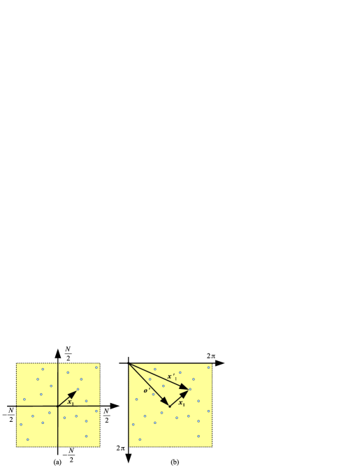
Fig. 1: Coordinate conversion for NUFFT. (a) coordinate system of the original plane (b) coordinate system of the plane for NUFFT. Blue circles indicate non-uniform sampled points.

NUFFT type 2 is defined as follows:

$$f(\bm{x}_{2}^{\prime})=\mathcal{{\rm NUFFT_{2}}}\biggl{[}F(\bm{m}_{f})\biggl{]}=\sum_{\bm{m}_{f}}F(\bm{m}_{f})\exp(i\pi\bm{m}_{f}\bm{x}_{2}^{\prime}),$$ (8)

where $f(\bm{x}_{2}^{\prime})$ is the non-uniform sampled plane. Note that we need to normalize the coordinate of the destination plane for the same reason as that of NUFFT₁. For more details, see [11].

Likewise, NU-ASM₂ is obtained as follows:

$$u_{2}(\bm{x}_{2}) = \mathcal{{\rm NUASM_{2}}}\biggl{[}u_{1}(\bm{m}_{1})\biggl{]},$$

$$= \mathcal{{\rm NUFFT_{2}}}\biggl{[}\mathcal{{\rm FFT}}\biggl{[}u_{1}(\bm{m}_{1})\biggl{]}H_{z,\Delta}(\bm{m}_{f})\biggl{]},$$

where $\Delta=1/(N^{\prime}\Delta_{1})$. $\bm{m}_{1}$ and $\bm{m}_{f}$ are uniform sampled. $\bm{x}_{2}$ is non-uniform sampled and the range is $\bm{x}_{2}\in[-N/2,N/2)\times[-N/2,N/2)$. The NUFFT₂ requires the range of the coordinate, $\bm{x}^{\prime}_{2}\in[0,2\pi)\times[0,2\pi)$. Therefore, we convert the coordinate system by $\bm{x}^{\prime}_{2}=2\pi(\bm{o}^{\prime}+\bm{x}_{2})/N$.

We obtain NU-ASM₃ by combining NU-ASM₁ and NU-ASM₂. In addition, using Eq.(5) instead of the transfer functions of NU-ASM, we can straightforwardly derive three types of NU-FRE, that is, NU-FRE₁, NU-FRE₂ and NU-FRE₃ .

Let us compare the NU-ASM and NU-FRE with Rayleigh-Sommerfeld (RS) diffraction. RS diffraction is rigorous scalar diffraction and is expressed as,

$$u_{2}({\bm{x}_{2}})=\frac{1}{2\pi}\int\!\!\int u_{1}(\bm{x}_{1})\left\{\frac{z}{r}(1-ikr)\frac{\exp(ikr)}{r^{2}}\right\}d{\bm{x}_{1}},$$ (10)

where $k$ is the wave number and $r=\sqrt{|\bm{x}_{1}-\bm{x}_{2}|^{2}+z^{2}}$. RS diffraction with non-uniform sampled planes is calculated by directly numerical integration, which has the complexity of $O(N^{4})$.

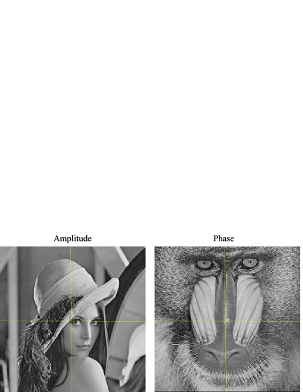
Fig. 2: Source plane with $256\times 256$ pixels. “Lenna” as the amplitude distribution of the source plane, and the image “Mandrill” as the phase distribution where the pixel value 0 corresponds to the phase value $-\pi/2$ and the pixel value 255 corresponds to the phase value $+\pi/2$.

We use Fig.2 as the non-uniform sampled source plane with $256\times 256$ pixels. The image “Lenna” is the amplitude distribution of the source plane, and the image “Mandrill” is the phase distribution where the pixel value 0 corresponds to the phase value $-\pi/2$ and the pixel value 255 corresponds to the phase value $+\pi/2$. The calculation condition is as follows: the wavelength is 500 nm and the sampling rate on the uniform-sampled destination plane is $\Delta_{2}=5\mu$m. The source plane is non-uniform-sampled, where the sampling rates on the first to fourth quadrants are $0.9\Delta_{2},0.8\Delta_{2},0.7\Delta_{2}$ and $\Delta_{2}$, respectively.

Figure 3(a) and (b) are the amplitude and phase on the diffracted result by RS diffraction at $z=8$mm. Figure 3(c) and (d) are the amplitude and phase on the diffracted result by NU-ASM₁. In Fig. 4, we measure the error of NU-ASM₁ and NU-FRE₁ to RS diffraction, which is the criteria, by the signal-to-noise ratio (SNR). At short distance propagation, the SNR of NU-ASM₁ is good quality, while that of NU-FRE₁ is poor quality. Whereas, at long distance propagation, the SNR of NU-ASM₁ is decreased because the band-limited transfer function of Eq.(4) has a small area, which is pointed out by Ref.[16]. While, the SNR of NU-FRE₁ is increased. The average calculation time of the NU-ASM₁ is about 46 ms, while that of RS diffraction is about 76 s. We use an Intel Core i7-2600S CPU and eight CPU threads, and multi-thread version of FFTW [17] as the FFT library.

Figure 5 shows diffracted results from a uniform-sampled source plane to non-uniform-sampled destination plane by RS diffraction and NU-ASM₂. We use Fig.2 as the uniform-sampled source plane at the sampling rate $\Delta_{1}=5\mu$m. The destination plane is non-uniform-sampled, where the sampling rates on the first to fourth quadrants are $0.9\Delta_{1},0.8\Delta_{1},0.7\Delta_{1}$ and $\Delta_{1}$, respectively. Figure 5(a) and (b) are the amplitude and phase on the diffracted result by RS diffraction at $z=8$mm. Figure 5(c) and (d) are the amplitude and phase on the diffracted result by NU-ASM₂. The SNR is maintained at approximately 32 dB.

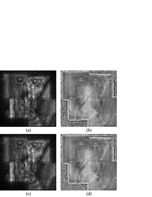
Fig. 3: Diffracted results of the amplitude and phase distribution by RS diffraction and NU-ASM. (a) amplitude by RS diffraction (b) phase by RS diffraction (c) amplitude by NU-ASM (d) phase by NU-ASM.

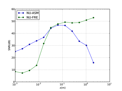
Fig. 4: Errors of NU-ASM₁ and NU-FRE₁ to RS diffraction by the signal-to-noise ratio (SNR).

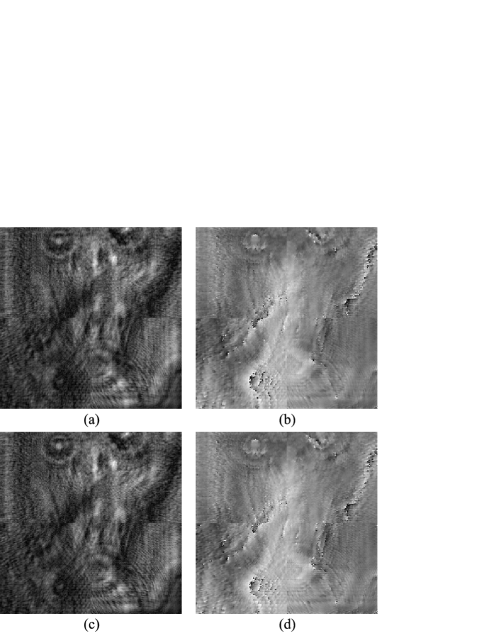
Fig. 5: Diffracted results of the amplitude and phase distribution by RS diffraction and NU-ASM. (a) amplitude by RS diffraction (b) phase by RS diffraction (c) amplitude by NU-ASM (d) phase by NU-ASM.

We conclude this work. This paper proposes the non-uniform sampled scalar diffractions, NU-ASM and NU-FRE, based on NUFFT. These diffractions are categorized into three types: type 1 is the diffraction from a non-uniform sampled source plane to a uniform sampled destination plane, the type 2 is the opposite situation of type 1; and type 3 is the diffraction between a non-uniform sampled source and destination planes. NU-ASM is suitable for the short propagation, while NU-FRE are suitable for the long propagation. In addition, the calculation times of NU-ASM and NU-FRE is faster than RS diffraction. In future, we will attempt to apply the non-uniform sampled scalar diffractions to CGH calculation, the design of optical elements, and optical encryption and watermarking. These diffraction calculations will be provided in our open-source library: CWO++ library [18].

This work is supported by the Ministry of Internal Affairs and Communications, Strategic Information and Communications R&D Promotion Programme (SCOPE)(09150542), Japan Society for the Promotion of Science (JSPS) KAKENHI (Young Scientists (B) 23700103) 2011, and the NAKAJIMA FOUNDATION.

References

- [1] J.W.Goodman, “Introduction to Fourier Optics (3rd ed.),” Robert & Company (2005).
- [2] K. Matsushima, “Shifted angular spectrum method for off-axis numerical propagation,” Opt. Express 18, 18453–18463 (2010).
- [3] L. Yaroslavsky, “Optical transforms in digital holography,” Proc. SPIE Holography 2005: International Conference on Holography, Optical Recording, and Processing of Information, 6252, 625216 (2006).
- [4] R. P. Muffoletto, J. M. Tyler, and J. E. Tohline, “Shifted Fresnel diffraction for computational holography,” Opt. Express 15, 5631–5640 (2007).
- [5] J. F. Restrepo and J. G. -Sucerquia, “Magnified reconstruction of digitally recorded holograms by Fresnel–Bluestein transform,” Appl. Opt. 49, 6430–6435 (2010) .
- [6] L. Bilevich and L. Yaroslavsky, “Fast DCT-based image convolution algorithms and application to image resampling and hologram reconstruction,” Proc. SPIE 7724, 77240N(2010).
- [7] T. Shimobaba, T. Kakue, N. Okada, M. Oikawa, Y. Yamaguchi, and T. Ito, “Aliasing-reduced Fresnel diffraction with scale and shift operations,” J.Opt. 15 075405 (2013).
- [8] S. Odate, C. Koike, H. Toba, T. Koike, A. Sugaya, K. Sugisaki, K. Otaki, and K. Uchikawa, “Angular spectrum calculations for arbitrary focal length with a scaled convolution,” Opt. Express 19, 14268–14276 (2011).
- [9] T. Shimobaba, K. Matsushima, T. Kakue, N. Masuda, and T. Ito, “Scaled angular spectrum method,” Opt. Lett. 37, 4128–4130 (2012).
- [10] X. Yu, T. Xiahui, Q. Yingxiong, P. Hao, and W. Wei, “Band-limited angular spectrum numerical propagation method with selective scaling of observation window size and sample number,” J. Opt. Soc. Am. A 29, 2415–2420 (2012).
- [11] L. Greengard and J. Y. Lee, “Accelerating the nonuniform fast Fourier transform, ” SIAM Rev. 46, 443–454 (2004).
- [12] T. Shimobaba, T. Kakue, N. Masuda and T. Ito, “Numerical investigation of zoomable holographic projection without a zoom lens,” J. Soc. Info. Disp. 20, 533–538 (2012).
- [13] T. Shimobaba, M. Makowski, T. Kakue, M. Oikawa, N. Okada, Y. Endo, R. Hirayama, and T. Ito, “Lensless zoomable holographic projection using scaled Fresnel diffraction,” Opt. Express (accepted).
- [14] T. Shimobaba, N. Masuda, Y. Ichihashi, and T. Ito, “Real-time digital holographic microscopy observable in multi-view and multi-resolution,” J. Opt. 12, 065402 (2010).
- [15] J. Weng, T. Shimobaba, N. Okada, H. Nakayama, M. Oikawa, N. Masuda, and T. Ito, , “Generation of real-time large computer generated hologram using wavefront recording method,” Opt. Express 20, 4018–4023 (2012).
- [16] X. Yu, T. Xiahui, Q. Y. Xiong, P. Hao, and W. Wei, “Wide-window angular spectrum method for diffraction propagation in far and near field,” Opt. Lett. 37, 4943–4945 (2012).
- [17] M. Frigo and S. G. Johnson, “FFTW: An adaptive software architecture for the FFT,” in Proc. 1998 IEEE Intl. Conf. on Acoustics, Speech, and Signal Processing (Institute of Electrical and Electronics Engineers, New York, 1998), 1381–1384.
- [18] T. Shimobaba, J. Weng, T. Sakurai, N. Okada, T. Nishitsuji, N. Takada, A. Shiraki, N. Masuda, and T. Ito, Comput. Phys. Commun. 183, 1124–1138 (2012).