A high-order accurate accelerated direct solver for acoustic scattering from surfaces

Abstract.

We describe an accelerated direct solver for the integral equations which model acoustic scattering from curved surfaces. Surfaces are specified via a collection of smooth parameterizations given on triangles, a setting which generalizes the typical one of triangulated surfaces, and the integral equations are discretized via a high-order Nyström method. This allows for rapid convergence in cases in which high-order surface information is available. The high-order discretization technique is coupled with a direct solver based on the recursive construction of scattering matrices. The result is a solver which often attains $O(N^{1.5})$ complexity in the number of discretization nodes $N$ and which is resistant to many of the pathologies which stymie iterative solvers in the numerical simulation of scattering. The performance of the algorithm is illustrated with numerical experiments which involve the simulation of scattering from a variety of domains, including one consisting of a collection of $1000$ ellipsoids with randomly oriented semiaxes arranged in a grid, and a domain whose boundary has $12$ curved edges and $8$ corner points.

1. Introduction

The manuscript describes techniques based on boundary integral equation formulations for numerically solving certain linear elliptic boundary value problems associated with acoustic scattering in three dimensions. There are three principal components to techniques of this type:

1. Reformulation. The boundary value problem is first reformulated as a system of integral equations, preferably involving operators which are well-conditioned when considered on spaces of integrable functions.

2. Discretization. The resulting integral operators are then discretized. High-order discretization methods are to be preferred to low-order schemes and the geometry of the domain under consideration is the principal consideration in producing high-order convergent approaches.

3. Accelerated Solver. The large dense system of linear algebraic equations produced through discretization must be solved. Accelerated solvers which exploit the mathematical properties of the underlying physical problems are required to solve most problems of interest.

For boundary value problems given on two-dimensional domains — which result in integral operators on planar curves — satisfactory approaches to each of these three tasks have been described in the literature. Uniquely solvable integral equation formulations of boundary value problems for Laplace’s equation and the Helmholtz equation are available [4, 30, 1, 19, 14]; many mechanisms for the high-order discretization of singular integral operators on planar curves are known [14, 25] and even operators given on planar curves with corner singularities can be discretized efficiency and to near machine precision accuracy [6, 5, 10, 23, 22]; finally, fast direct solvers which often have run times which are asymptotically optimal in the number of discretization nodes $N$ have been constructed [27, 15, 33, 3, 16, 12, 20, 24].

For three-dimensional domains, the state of affairs is much less satisfactory. In this case, the integral operators of interest are given on curved surfaces which greatly complicates problems (2) and (3) above. Problem (2) requires the evaluation of large numbers of singular integrals given on curved regions. Standard mechanisms for addressing this problem, like the Duffy transform followed by Gaussian quadrature, are limited in their applicability (see [7] for a discussion). Most fast solvers (designed to address problem (3)) are based on iterative methods and can fare poorly when the surface under consideration exhibits complicated geometry. For example, a geometry consisting of a $2\times 2\times 2$ grid of ellipsoids ($1536$ discretization points per ellipsoid) bounded by a box two wavelengths in size takes over $1000$ GMRES iterations to get the residual below $10^{-3}$ (see Figure 6 and Remark 6.1). Moreover, iterative methods are unable to efficiently handle problems with multiple right hand sides that arise frequently in design problems.

In this manuscript, we describe our contributions towards providing a remedy to problems (2) and (3). We consider scattering problems that arise in applications such as sonar and radar where the goal is to find the scattered field at a set of locations $\Gamma_{\rm out}$ generated when an incident wave sent from locations $\Gamma_{\rm in}$ hit an object or collections of objects (whose surface we denote $\Gamma$), cf. Fig. 1(a). The locations of the source and target points are known and typically given by the user. In this context, we present an efficient high-order accurate method for constructing a scattering matrix $\mathsf{S}$ which maps the incident field generated by the given sources on $\Gamma_{\rm in}$ to a set of induced charges on $\Gamma$ that generate the scattered field on $\Gamma_{\rm out}$. A crucial component to constructing $\mathsf{S}$ is solving a boundary integral equation defined on $\Gamma$. A recently developed high order accurate discretization technique for integral equations on surfaces [7, 8] is used. This discretization has proven to be effective for Laplace and low frequency scattering problems. Since many scattering problems of interest involve higher frequencies and complicated geometries, a large number of discretization points are typically required to achieve high accuracy, even for high-order methods. In consequence, it would be infeasible to solve the resulting linear systems using dense linear algebra (e.g., Gaussian elimination). As a robust alternative to the commonly used iterative solvers (whose convergence problems in the present context was previously discussed), we propose the use of a direct solver that exploits the underlying structure of the matrices of interest to construct an approximation to the scattering matrix $\mathsf{S}$. Direct solvers have several benefits over iterative solvers: (i) the computational cost does not depend on the spectral properties of the system, (ii) each additional incoming field can be processed quickly, (iii) the amount of memory required to store the scattering matrix scales linearly with the number of discretization points.

1.1. Model problems

The solution technique presented is applicable to many boundary integral equations that arise in mathematical physics but we limit our discussion to the boundary value problems presented in this section.

Let $\Omega$ denote a scattering body, or a union of scattering bodies; Figures 6, 7, 8, 9, and 11 of Section 6 illustrate some specific domains of interest. Let $\Gamma=\partial\Omega$ denote the surface of the body (or bodies). We are interested in finding the scattered field $u$ off $\Omega$ for a given incident wave $u_{\rm in}$. Specifically this involves solving either an exterior Dirichlet problem for sound-soft scatterers

$$\left\{\begin{aligned} \Delta u+\kappa^{2}u=&\ 0\qquad&&\mbox{ in }\Omega^{c},\\ u=&\ g\qquad&&\mbox{ on }\Gamma,\\ \frac{\partial u}{\partial r}-i\kappa u=&\ O\left(\frac{1}{r}\right)\qquad&&\mbox{ as }r\to\infty,\end{aligned}\right.$$ (DBVP)

where $g=-u_{\rm in}$, or an exterior Neumann problem for sound-hard scatterers

$$\left\{\begin{aligned} \Delta u+\kappa^{2}u=&\ 0\qquad&&\mbox{ in }\Omega^{c},\\ \frac{\partial u}{\partial\eta}=&\ g\qquad&&\mbox{ on }\Gamma,\\ \frac{\partial u}{\partial r}-i\kappa u=&\ O\left(\frac{1}{r}\right)\qquad&&\mbox{ as }r\to\infty,\end{aligned}\right.$$ (NBVP)

where $\eta$ is the outwards point unit normal vector to $\Gamma$, and where $g=-\partial_{\eta}u_{\rm in}$.

1.2. Outline

The paper proceeds by introducing the integral formulations for each choice of boundary condition in Section 2. Section 3 presents a high order accurate technique for discretizing the integral equations. Section 4 formally defines a scattering matrix and describes a method for constructing an approximation of the scattering matrix. Section 5 describes an accelerated technique for constructing the scattering matrix that often has asymptotic cost of $O(N^{3/2})$ (providing the scattering body and the wave-length of the radiating field are kept constant as $N$ increases). Section 6 presents the results of several numerical experiments which demonstrate the properties of the proposed solver.

2. Integral equation formulations of linear elliptic boundary value problems

The reformulation of the boundary value problems in Section 1.1 as integral equations involves the classical single and double layer operators

$$\begin{split}S_{\kappa}f(x)&=\int\hskip-7.0pt\int_{\Gamma}G_{\kappa}(x,y)f(y)ds(y),\\ D_{\kappa}f(x)&=\int\hskip-7.0pt\int_{\Gamma}\eta_{y}\cdot\nabla_{y}G_{\kappa}(x,y)f(y)ds(y)\ \ \mbox{and}\\ D_{\kappa}^{*}f(x)&=\int\hskip-7.0pt\int_{\Gamma}\eta_{x}\cdot\nabla_{x}G_{\kappa}(x,y)f(y)ds(y)\end{split}$$ (2.1)

where $G_{\kappa}(x,y)$ is the free space Green’s function

$$G_{\kappa}(x,y)=\frac{\exp\left(i\kappa\left|x-y\right|\right)}{\left|x-y\right|}$$

associated with the Helmholtz equation at wavenumber $\kappa$ and where $\eta_{p}$ denotes the outward-pointing unit normal to the surface $\Gamma$ at the point $p$.

The reformulation of (DBVP) and (NBVP) is not entirely straightforward because of the possibility of spurious resonances. That is, for certain values of the wavenumber $\kappa$, the naïve integral equation formulations of (DBVP) and (NBVP) lead to operators with nontrivial null-spaces, even though the original boundary value problems are well-posed. The wave-numbers $\kappa$ for which this occurs are called spurious resonances. Complications arise due to the existence of multiple solutions at a resonance. An additional (and perhaps more serious) problem is that for values of $\kappa$ close to resonant values, the integral operators (2.1) become ill-conditioned.

2.1. The boundary integral formulation for Dirichlet boundary values problems

The double layer representation

$$u(x)=D_{\kappa}\sigma(x).$$

of the solution of (DBVP) leads to the second kind integral equation

$$\frac{1}{2}\sigma(x)+D_{\kappa}\sigma(x)=g(x).$$

As is well known, this integral equation is not be uniquely solvable in the event that the eigenproblem

$$\begin{split}\Delta u+\kappa^{2}u=0\ \ \ &\mbox{ in }\Omega\\ \frac{\partial u}{\partial\eta}=0\ \ \ &\mbox{ on }\Gamma\\ \end{split}$$

admits a nontrivial solution. A uniquely solvable integral equation can be obtained by choosing to represent the solution as

$$u(x)=D_{\kappa}\sigma(x)+i|\kappa|S_{\kappa}\sigma(x);$$ (2.2)

see, for instance, [28, 14]. This leads to the integral equation

$$\frac{1}{2}\sigma(x)+D_{\kappa}\sigma(x)+i|\kappa|S_{\kappa}\sigma(x)=g(x),$$ (2.3)

which is sometimes referred to as the Combined Field Integral Equation (CFIE). We make use of the CFIE to solve the problem (DBVP) in this article.

2.2. The boundary integral formulation for Neumann boundary values problems

The single layer representation

$$u=S_{\kappa}\sigma.$$

of the solution of (NBVP) leads to the second kind integral equation

$$\frac{1}{2}\sigma(x)+D_{\kappa}^{*}\sigma(x)=g(x).$$ (2.4)

Once again the equation (2.4) is not necessarily uniquely solvable — when the eigenproblem

$$\begin{split}\Delta u+\kappa^{2}u=0\ \ \ &\mbox{ in }\Omega\\ u=0\ \ \ &\mbox{ on }\Gamma\\ \end{split}$$ (2.5)

has nontrivial solutions (that is, when $\kappa$ is a resonant wavenumber), the operator appearing on the right-hand side of (2.4) is not invertible. Since the focus of this article is on the discretization of integral operators and the rapid inversion of the resulting matrices, we simply avoid wavenumbers $\kappa$ for which spurious resonances exist. Appendix A presents a robust integral equation formulation which is suitable for use by the solver of this paper. We forgo its use here in order to reduce the complexity of the presentation.

3. A Nyström method for the discretization of integral equations on surfaces

In this work, we use a modified Nyström method for the discretization of the integral operators (2.1) of the proceeding section. Our approach differs from standard Nyström methods in two important ways:

1. It captures the $L^{2}$ action of an operator rather than its pointwise behavior. Among other advantages, this means that the approach results in well-conditioned operators in the case of Lipschitz domains.

2. A highly accurate mechanism for evaluating the singular integrals which arise in Nyström discretization whose cost is largely independent of the geometry of the surface is employed. This is in contrast to standard methods for the evaluation of the singular integrals arising from the Nyström discretization of integral operators on surfaces which involve constants which depend on the geometry of the domain.

This manuscript gives a cursory account of the method. A detailed description can be found in [7] and a discussion of the advantages of $L^{2}$ discretization over standard Nyström and collocation methods can be found in [6].

3.1. Decompositions and discretization quadratures.

We define a decomposition $D$ of a surface $\Gamma\subset\mathbb{R}^{3}$ to be a finite sequence

$$\{\rho_{j}:\Delta^{1}\to\Gamma\}_{j=1}^{m}$$

of smooth mappings given on the simplex

$$\Delta^{1}=\left\{\left(x,y\right)\in\mathbb{R}^{2}\ :\ 0\leq x\leq 1,\ 0\leq y\leq 1-x\right\}$$

with non-vanishing Jacobian determinants such that the sets

$$\rho_{1}(\Delta^{1}),\rho_{2}(\Delta^{1}),\ldots,\rho_{m}(\Delta^{1})$$

form a disjoint union of $\Gamma$.

We call a quadrature rule $\{x_{1},\ldots,x_{l},w_{1},\ldots,w_{l}\}$ on $\Delta^{1}$ with positive weights which integrates all elements of the space $\mathscr{P}_{N}$ of polynomials of degree less than or equal to $2N$ on the simplex $\Delta^{1}$ a discretization quadrature. Such a rule is called Gaussian if the length $l$ of the rule is equal to $(N+1)\cdot(N+2)/2$. That is, a Gaussian rule is one whose length is equal to the dimension of the space of polynomials of degree less than or equal to $N$ but which integrates polynomials of degree less than or equal to $2N$. For the most part, Gaussian quadratures on triangles are not available. In the experiments of this paper, we used quadrature rules constructed via a generalization of the procedure of [9]. Table 1 lists the properties of the discretization quadrature rules used in this paper and compare their lengths to the size of a true Gaussian quadrature.

Discretization order	$N$	4	6	8	10	12	16
Integration order	$2N$	8	12	16	20	24	32
Length of a true Gaussian quadrature	$(N+1)(N+2)/2$	15	28	45	66	91	153
Length of the quadrature that we use	$l$	17	32	52	82	112	192

Table 1. The properties of the quadratures used in this paper. We compare the length of an ideal (hypothetical) Gaussian quadrature to the quadrature that we actually have.

3.2. Discretizations of integral operators.

We now associate with a decomposition

$$D=\{\rho_{j}:\Delta^{1}\to\Gamma\}_{j=1}^{m}$$

and a discretization quadrature $\{x_{1},\ldots,x_{l},w_{1},\ldots,w_{l}\}$ a scheme for the discretization of certain integral operators. We begin by letting $S$ be the subspace of $L^{2}(\Gamma)$ consisting of all functions $f$ which are pointwise defined on $\Gamma$ and such that for each $j=1,\ldots,m$ the function

$$f(\rho_{j}(x))\left|d\rho_{j}(x)^{*}d\rho_{j}(x)\right|^{1/2}$$

is a polynomial of order $N$ on $\Delta^{1}$. Denote by $P$ be the projection of $L^{2}(\Gamma)$ onto the subspace $S$ and let $\Phi:S\to\mathbb{C}^{ml}$ be a mapping which takes $f\in S$ to a vector with entries

$$f\left(\rho_{j}(x_{i})\right)\sqrt{w_{i}}\left|d\rho_{j}(\rho_{j}(x_{i}))^{*}d\rho_{j}(\rho_{j}(x_{i}))\right|^{1/4},\ \ \ j=1,\ldots,m,\ \ i=1,\ldots,l.$$

The ordering of the entries of $\Phi(f)$ is irrelevant. Suppose that $T:L^{2}(\Gamma)\to L^{2}(\Gamma)$ is of the form

$$Tf(x)=\int\hskip-7.0pt\int_{\Gamma}K(x,y)f(y)ds(y),$$ (3.1)

with $K$ a linear combination of the kernels listed in (2.1). Let $A$ denote the $ml\times ml$ matrix which commutes the discretization of the operator $T$ induced by the specified decomposition and discretization quadrature as specified in the diagram (3.2).

$$\begin{CD}S\subset L^{2}(\Gamma)@>{PT}>{}>S\subset L^{2}(\Gamma)\\ @V{}V{\Phi}V@ VV\Phi V\\ \mathbb{C}^{ml}@>{A}>{}>\mathbb{C}^{ml}\end{CD}$$ (3.2)

3.3. Quadrature.

Forming the matrix $A$ which appears the diagram (3.2) is an exercise in numerical quadrature. Let $x$ be a discretization node on $\Delta$ and let $w$ be the corresponding weight. The $l$ entries of the matrix $A$ in (3.2) associated with the mapping $\rho_{j}$ and the point $\rho_{i}(x)$ must map the scaled values

$$f(\rho_{j}(x_{1}))|d\rho^{*}_{j}(x_{k})d\rho_{j}(x_{k})|^{1/4}\sqrt{w_{k}},\qquad k=1,2,\dots,l,$$ (3.3)

of the function $f$ at the images of the discretization quadrature nodes under $\rho_{j}$ to the value of the integral

$$\int\hskip-7.0pt\int_{\Delta^{1}}K(\rho_{i}(x),\rho_{j}(y))f(\rho_{j}(y))|d\rho^{*}_{j}(y)d\rho_{j}(y)|^{1/2}\sqrt{w}\ dy.$$ (3.4)

The manner in which this vector is formed depends on the location of the point $\rho_{i}(x)$ vis-à-vis the patch $\rho_{j}(\Delta^{1})$. Let $B$ denote the ball of minimum radius containing $\Gamma$ and $2B$ denote the ball with the same center as $B$ but with twice the radius. Then we say that a point $x$ is well-separated from a surface $\Gamma$ if $x$ is outside of $2B$, and we say that $x$ is near $\Gamma$ if $x$ is inside of the ball $2B$ but not on the surface $\Gamma$.

3.3.1. Smooth regime.

When the point $\rho_{i}(x)$ is well-separated from $\rho_{j}(\Delta^{1})$ the kernel $K$ is smooth and the discretization quadrature can be used to evaluate the integral (3.4). In this case, we take the $l$ entries of the matrix $A$ to be

$$K(\rho_{i}(x),\rho_{j}(x_{k}))\left|d\rho_{j}^{*}(x_{k})d\rho_{j}(x_{k})\right|^{1/4}\sqrt{w}\sqrt{w_{k}},\ \ \ k=1,2,\ldots,l.$$ (3.5)

3.3.2. Near regime.

When $\rho_{i}(x)$ is near $\rho_{j}(\Delta^{1})$, formula (3.5) may not achieve sufficient accuracy. Thus, we adaptively form a quadrature with nodes and weights

$$u_{1},\ldots,u_{m},r_{1},\ldots,r_{m}$$

sufficient to evaluate the nearly singular integrals which arise and apply an interpolation matrix $I$ which takes the scaled values (3.3) of the function $f$ at the nodes of the discretization quadrature to its scaled values at the nodes of the adaptive quadrature. The vector of entries of $A$ is given by the product of the vector of values of the kernel evaluated at the adaptive quadrature nodes with the matrix $I$. As in the scheme of [7], the adaptive quadrature is formed in such a way that the matrix $I$ has special structure — it is a product of block diagonal matrices — which allows it to be applied efficiently.

3.3.3. Singular regime.

When the target node lies on the surface $\rho_{j}(\Delta^{1})$, the integral (3.4) is singular and its evaluation becomes quite difficult. The typical approach to the evaluation of integrals of this form is to apply the Duffy transform or polar coordinate transform in order to remove the singularity of the kernel. Once this has been done, quadratures for smooth functions (for instance, product Legendre quadratures) are typically applied.

While the such schemes are exponentially convergent, they can be extremely inefficient. The difficulty is that the functions resulting from the change of variables can have poles close to the integration domain. For instance, if a polar coordinate transform is applied, the singular integrals which must be evaluated take the form

$$\int_{0}^{2\pi}\hskip 1.00006pt\int_{0}^{{R}(\theta)}\left(q_{-1}(\theta)+q_{0}(\theta)r+q_{1}(\theta)r^{2}+q_{2}(\theta)r^{3}+\cdots\ \right)dr\hskip 1.00006ptd\theta$$ (3.6)

where the function $R(\theta)$ gives a parameterization of the integration domain $\Delta^{1}$ in polar coordinates and each $q_{j}(\theta)$ is a quotient form

$$\frac{r_{j}(\theta)}{l(\theta)^{\alpha}},$$

where $\alpha$ is a positive constant dependent on the order $j$ and the kernel under consideration, $r_{j}(\theta)$ is a trigonometric polynomial of finite order, and $l(\theta)$ is a function which depends on the parameterization $\rho_{j}$. More specifically, if

$$\xi_{1}=\frac{\partial\rho_{j}(x_{1},x_{2})}{\partial x_{1}}\ \ \ \mbox{ and }\ \ \ \xi_{2}=\frac{\partial\rho_{j}(x_{1},x_{2})}{\partial x_{2}},$$

then the function $l(\theta)$ is given by

$$l(\theta)=\sqrt{\lambda\cos^{2}(\theta)+2\gamma\cos(\theta)\sin(\theta)+\lambda^{-1}\sin^{2}(\theta)}$$

where

$$\cos(\gamma)=\frac{\xi_{1}\cdot\xi_{2}}{\left|\xi_{1}\right|\left|\xi_{2}\right|}\ \ \ \mbox{ and }\ \ \ \lambda=\frac{\left|\xi_{1}\right|}{\left|\xi_{2}\right|}.$$

Obviously, the function $l(\theta)$ can have zeros close to the real axis.

The approach used in this paper — and described in [7] — calls for first applying a change of variables in order to ensure that the mapping $\rho_{j}$ is conformal at the target node. Then the function $l(\theta)$ is a constant which does not depend on $\theta$ and the integrand simplifies considerably. The unfortunate side effect of applying this change of variables is that the integration domain is no longer the standard simplex $\Delta^{1}$ but rather an arbitrary triangle. Now the integral which must be evaluated takes the form

$$\int_{0}^{2\pi}\hskip 1.00006pt\int_{0}^{\tilde{R}(\theta)}\left(\tilde{q}_{-1}(\theta)+\tilde{q}_{0}(\theta)r+\tilde{q}_{1}(\theta)r^{2}+\tilde{q}_{2}(\theta)r^{3}+\cdots\ \right)dr\hskip 1.00006ptd\theta$$ (3.7)

with the $\tilde{q_{j}}$ trigonometric polynomials of finite order. The function $\tilde{R}(\theta)$ can have poles close to the integration domain, however. We combat this problem by precomputing a collection of quadrature rules designed to integrate smooth functions on arbitrary triangles and apply them to evaluate the integrals (3.7). The performance of this approach is described in [7]; in one example of that paper, the standard approach of applying a change of variables followed by Gauss-Legendre quadrature required more than $100,000$ quadrature nodes to accurately evaluate the singular integrals arising from a boundary value problem while the precomputed rules used here and in that paper required less than $1,000$ nodes.

4. Scattering matrices as a numerical tool

This section describes the concept of a scattering matrix, first from a physical perspective, and then the corresponding linear algebraic interpretation. It also informally describes how to build approximate scattering matrices computationally. A rigorous description is given in Section 5.

4.1. The scattering operator

We consider a “sound-soft” scattering formulation illustrated in Figure 1. We are given a charge distribution $s_{\rm in}$ on a contour $\Gamma_{\rm in}$ (the radiation “source”) that generates an incoming field $g$ on the scatterer $\Gamma$. The incoming field on the scatterer induces an outgoing field $u$ that satisfies (DBVP). Our objective is to computationally construct $u_{\rm out}$, the restriction of the outgoing field to the specified contour $\Gamma_{\rm out}$, which represents the “antenna.” To solve (DBVP), we use the combined field formulation (2.2). In other words, we represent the outgoing field via a distribution $\sigma$ of “induced sources” on the contour $\Gamma$. The map we seek to evaluate can be expressed mathematically as

$$\begin{array}[]{ccccccccc}u_{\rm out}&=&T_{\rm out}&T_{\Gamma}^{-1}&T_{\rm in}&s_{\rm in},\\[5.69054pt] \mbox{{outgoing field on }}\Gamma_{\rm out}&&&&&\mbox{{given charges on }}\Gamma_{\rm in}\end{array}$$ (4.1)

where $T_{\rm in}\,\colon\,L^{2}(\Gamma_{\rm in})\rightarrow L^{2}(\Gamma)$ is the operator

$$[T_{\rm in}s_{\rm in}](x)=\int_{\Gamma_{\rm in}}G_{\kappa}(x,y)s_{\rm in}(y)ds(y),\qquad x\in\Gamma,$$

$T_{\Gamma}\,\colon\,L^{2}(\Gamma)\rightarrow L^{2}(\Gamma)$ is the operator

$$[T_{\Gamma}g](x)=\frac{1}{2}g(x)+D_{\kappa}g(x)+i|\kappa|S_{\kappa}g(x),\qquad x\in\Gamma,$$ (4.2)

and $T_{\rm out}\,\colon\,L^{2}(\Gamma)\rightarrow L^{2}(\Gamma_{\rm out})$ is the operator

$$[T_{\rm out}\sigma](x)=\int_{\Gamma}G_{\kappa}(x,y)\sigma(y)ds(y)+\int_{\partial\Omega}\partial_{\nu_{y}}G_{\kappa}(x,y)\sigma(y)ds(y),\qquad x\in\Gamma_{\rm out}.$$

Observe that since $T_{\Gamma}$ is an invertible second kind integral operator, its inverse has singular values bounded away from zero.

Given a finite precision $\varepsilon>0$, we say that an operator $S\,\colon\,L^{2}(\Gamma)\rightarrow L^{2}(\Gamma)$ is a “scattering operator” for $\Gamma$ to within precision $\varepsilon$ when

$$\|T_{\rm out}\,T_{\Gamma}^{-1}\,T_{\rm in}-T_{\rm out}\,S\,T_{\rm in}\|\leq\varepsilon.$$

It turns out that the operators $T_{\rm in}$ and $T_{\rm out}$ have rapidly decaying singular values. Let $P_{\rm in}^{(k)}$ denote the orthogonal projection onto the set of $k$ leading left singular vectors of $T_{\rm in}$, and let $P_{\rm out}^{(k)}$ denote the orthogonal projection onto the set of $k$ leading right singular vectors of $T_{\rm out}$. Then

$$\|T_{\rm out}P_{\rm out}^{(k)}-T_{\rm out}\|\leq\sigma_{k+1}(T_{\rm out})\qquad\mbox{and}\qquad\|T_{\rm in}P_{\rm in}^{(k)}-T_{\rm in}\|\leq\sigma_{k+1}(T_{\rm in}).$$

It follows that if we define an approximate scattering operator $S$ via

$$S=P_{\rm out}^{(k)}\,T_{\Gamma}^{-1}\,P_{\rm in}^{(k)},$$ (4.3)

then the approximation error

$$\|T_{\rm out}\,T_{\Gamma}^{-1}\,T_{\rm in}-T_{\rm out}\,P_{\rm out}^{(k)}\,T_{\Gamma}^{-1}\,P_{\rm in}^{(k)}\,T_{\rm in}\|$$

converges to zero very rapidly as $k$ increases.

(a)		(b)

Figure 1. Geometry of the scattering problem in Section 4. The scattering surface is $\Gamma$. (a) The radiation source $\Gamma_{\rm in}$ is different from the antenna $\Gamma_{\rm out}$. (b) The typical geometry considered with $\Gamma_{\rm in}=\Gamma_{\rm out}$. The scattering matrix generated by this geometry is the “complete” scattering matrix in the sense that any incoming field can be handled (as long as the radiation source is not inside $\Gamma_{\rm in}$), and the full radiated field can be obtained.

4.2. Definition of a discrete scattering matrix

The continuum scattering problem described in Section 4.1 has a direct linear algebraic analog for the discretized equations. Forming the Nyström discretization of the three operators in (4.1), we obtain the map

$$\begin{array}[]{ccccccccc}\bm{u}_{\rm out}&=&\mathsf{A}_{\rm out}&\mathsf{A}^{-1}&\mathsf{A}_{\rm in}&\bm{s}_{\rm in}.\\[5.69054pt] N_{\rm out}\times 1&&N_{\rm out}\times N&N\times N&N\times N_{\rm in}&N_{\rm in}\times 1\end{array}$$ (4.4)

Suppose that $\mathsf{A}$ is an $N\times N$ matrix, and let $k_{1}$ denote a bound on the $\varepsilon$-ranks of $\mathsf{A}_{\rm out}$ and $\mathsf{A}_{\rm in}$. Then form matrices $\hat{\mathsf{U}}_{1}$ and $\hat{\mathsf{V}}_{1}$ (the reason for the subscripts will become clear shortly) of size $N\times k_{1}$ such that

$$\|\mathsf{A}_{\rm in}-\hat{\mathsf{U}}_{1}\,\hat{\mathsf{U}}_{1}^{\dagger}\,\mathsf{A}_{\rm in}\|\leq\varepsilon,\qquad\mbox{}\qquad\|\mathsf{A}_{\rm out}-\mathsf{A}_{\rm out}\,(\hat{\mathsf{V}}_{1}\hat{\mathsf{V}}_{1}^{\dagger})^{*}\|\leq\varepsilon$$

where a matrix with the superscript $\dagger$ denotes the pseudo-inverse of the matrix. In other words, the columns of $\hat{\mathsf{U}}_{1}$ span the column space of $\mathsf{A}_{\rm in}$ and the columns of $\hat{\mathsf{V}}_{1}$ span the row space of $\mathsf{A}_{\rm out}$. Then the map (4.4) can be approximated as

$$\begin{array}[]{ccccccccc}\bm{u}_{\rm out}&=&\bigl{(}\mathsf{A}_{\rm out}\,(\hat{\mathsf{V}}_{1}^{\dagger})^{*}\bigr{)}&\mathsf{S}_{1}&\bigl{(}\hat{\mathsf{U}}_{1}^{\dagger}\,\mathsf{A}_{\rm in}\bigr{)}&\bm{s}_{\rm in},\\[5.69054pt] N_{\rm out}\times 1&&N_{\rm out}\times k_{1}&k_{1}\times k_{1}&k_{1}\times N_{\rm in}\end{array}$$ (4.5)

where

$$\mathsf{S}_{1}=\hat{\mathsf{V}}_{1}^{*}\,\mathsf{A}^{-1}\,\hat{\mathsf{U}}_{1}.$$ (4.6)

The $k_{1}\times k_{1}$ matrix $\mathsf{S}_{1}$ is the discrete analog of the continuum scattering matrix $S$ for $\Gamma$ defined by (4.3).

4.3. Hierarchical construction of discrete scattering matrices

Observe that direct evaluation of the definition (4.6) of $\mathsf{S}_{1}$ via, e.g., Gaussian elimination, would be very costly since $\mathsf{A}$ is dense, and $N$ could potentially be large (much larger than $k_{1}$). To avoid this expense, we will build $\mathsf{S}_{1}$ via an accelerated hierarchical procedure. As a first step, we let the entire domain $\Gamma=\Gamma_{1}$ denote the root of the tree, and split $\Gamma_{1}$ into two disjoint halves, cf. Figure 2(b),

$$\Gamma_{1}=\Gamma_{2}\cup\Gamma_{3}.$$ (4.7)

Let $n_{2}$ and $n_{3}$ denote the number of collocation points in $\Gamma_{2}$ and $\Gamma_{3}$, respectively. The idea is now to form scattering matrices $\mathsf{S}_{2}$ and $\mathsf{S}_{3}$ for the two halves, and then form $\mathsf{S}_{1}$ by “merging” these smaller scattering matrices. To formalize, split the matrix $\mathsf{A}$ into blocks to conform with the partitioning (4.7),

$$\mathsf{A}=\left[\begin{array}[]{cc}\mathsf{A}_{2,2}&\mathsf{A}_{2,3}\\ \mathsf{A}_{3,2}&\mathsf{A}_{3,3}\end{array}\right].$$

The off-diagonal blocks $\mathsf{A}_{2,3}$ and $\mathsf{A}_{3,2}$ have very rapidly decaying singular values, which means that they can be factored

$$\begin{array}[]{cccccc}\mathsf{A}_{2,3}&=&\hat{\mathsf{U}}_{2}&\tilde{\mathsf{A}}_{2,3}&\hat{\mathsf{V}}_{3}^{*},\\ n_{2}\times n_{3}&&n_{2}\times k_{2}&k_{2}\times k_{3}&k_{3}\times n_{3}\end{array}$$ (4.10)

$$\begin{array}[]{cccccc}\mathsf{A}_{3,2}&=&\hat{\mathsf{U}}_{3}&\tilde{\mathsf{A}}_{3,2}&\hat{\mathsf{V}}_{2}^{*}.\\ n_{3}\times n_{2}&&n_{3}\times k_{3}&k_{3}\times k_{2}&k_{2}\times n_{2}\end{array}$$ (4.13)

The matrices $\{\hat{\mathsf{U}}_{2},\,\hat{\mathsf{U}}_{3}\}$ and $\{\hat{\mathsf{V}}_{2},\,\hat{\mathsf{V}}_{3}\}$ are additionally assumed to span the column spaces of $\mathsf{A}_{\rm in}$ and $\mathsf{A}_{\rm out}^{*}$, in the sense that there exist “small” matrices $\mathsf{U}_{1}$ and $\mathsf{V}_{1}$ such that

$$\begin{array}[]{cccccc}\hat{\mathsf{U}}_{1}&=&\left[\begin{array}[]{cc}\hat{\mathsf{U}}_{2}&\mathsf{0}\\ \mathsf{0}&\hat{\mathsf{U}}_{3}\end{array}\right]&\mathsf{U}_{1},\\ N\times k_{1}&&N\times(k_{2}+k_{3})&(k_{2}+k_{3})\times k_{1}\end{array}\quad\mbox{and}\quad\begin{array}[]{cccccc}\hat{\mathsf{V}}_{1}&=&\left[\begin{array}[]{cc}\hat{\mathsf{V}}_{2}&\mathsf{0}\\ \mathsf{0}&\hat{\mathsf{V}}_{3}\end{array}\right]&\mathsf{V}_{1}.\\ N\times k_{1}&&N\times(k_{2}+k_{3})&(k_{2}+k_{3})\times k_{1}\end{array}$$ (4.14)

Inserting (4.10), (4.13), and (4.14) into (4.6), we find

$$\mathsf{S}_{1}=\mathsf{V}_{1}^{*}\left[\begin{array}[]{cc}\hat{\mathsf{V}}_{2}^{*}&\mathsf{0}\\ \mathsf{0}&\hat{\mathsf{V}}_{3}^{*}\end{array}\right]\left[\begin{array}[]{cc}\mathsf{A}_{2,2}&\hat{\mathsf{U}}_{2}\tilde{\mathsf{A}}_{2,3}\hat{\mathsf{V}}_{3}^{*}\\ \hat{\mathsf{U}}_{3}\tilde{\mathsf{A}}_{3,2}\hat{\mathsf{V}}_{2}^{*}&\mathsf{A}_{3,3}\end{array}\right]^{-1}\left[\begin{array}[]{cc}\hat{\mathsf{U}}_{2}&\mathsf{0}\\ \mathsf{0}&\hat{\mathsf{U}}_{3}\end{array}\right]\mathsf{U}_{2}.$$ (4.15)

Using the Woodbury formula for matrix inversion (see Lemma 5.1), it can be shown that

$$\left[\begin{array}[]{cc}\hat{\mathsf{V}}_{2}^{*}&\mathsf{0}\\ \mathsf{0}&\hat{\mathsf{V}}_{3}^{*}\end{array}\right]\left[\begin{array}[]{cc}\mathsf{A}_{2,2}&\hat{\mathsf{U}}_{2}\tilde{\mathsf{A}}_{2,3}\hat{\mathsf{V}}_{3}^{*}\\ \hat{\mathsf{U}}_{3}\tilde{\mathsf{A}}_{3,2}\hat{\mathsf{V}}_{2}^{*}&\mathsf{A}_{3,3}\end{array}\right]^{-1}\left[\begin{array}[]{cc}\hat{\mathsf{U}}_{2}&\mathsf{0}\\ \mathsf{0}&\hat{\mathsf{U}}_{3}\end{array}\right]=\left[\begin{array}[]{cc}\mathsf{I}&\mathsf{S}_{2}\tilde{\mathsf{A}}_{2,3}\\ \mathsf{S}_{3}\tilde{\mathsf{A}}_{3,2}&\mathsf{I}\end{array}\right]^{-1}\,\left[\begin{array}[]{cc}\mathsf{S}_{2}&\mathsf{0}\\ \mathsf{0}&\mathsf{S}_{3}\end{array}\right]$$ (4.16)

where $\mathsf{S}_{2}$ and $\mathsf{S}_{3}$ are the scattering matrices for $\Gamma_{2}$ and $\Gamma_{3}$, respectively. The matrices $\mathsf{S}_{2}$ and $\mathsf{S}_{3}$ are given by the following formulas

$$\mathsf{S}_{2}=\hat{\mathsf{V}}_{2}^{*}\mathsf{A}_{2,2}^{-1}\hat{\mathsf{U}}_{2},\qquad\mbox{and}\qquad\mathsf{S}_{3}=\hat{\mathsf{V}}_{3}^{*}\mathsf{A}_{3,3}^{-1}\hat{\mathsf{U}}_{3}.$$ (4.17)

Combining (4.15) and (4.16), we obtain the formula

$$\mathsf{S}_{1}=\mathsf{V}_{1}^{*}\left[\begin{array}[]{cc}\mathsf{I}&\mathsf{S}_{2}\tilde{\mathsf{A}}_{2,3}\\ \mathsf{S}_{3}\tilde{\mathsf{A}}_{3,2}&\mathsf{I}\end{array}\right]^{-1}\,\left[\begin{array}[]{cc}\mathsf{S}_{2}&\mathsf{0}\\ \mathsf{0}&\mathsf{S}_{3}\end{array}\right]\mathsf{U}_{1}.$$ (4.18)

The upside here is that in order to evaluate (4.18), we only need to invert a matrix of size $(k_{2}+k_{3})\times(k_{2}+k_{3})$, whereas (4.6) requires inversion of a matrix of size $N\times N$. The downside is that we are still left with the task of inverting $\mathsf{A}_{2,2}$ and $\mathsf{A}_{3,3}$ to evaluate $\mathsf{S}_{2}$ and $\mathsf{S}_{3}$ via (4.17). Now, to reduce the cost of constructing $\mathsf{S}_{2}$ and $\mathsf{S}_{3}$, we further sub-divide

$$\Gamma_{2}=\Gamma_{4}\cup\Gamma_{5},\qquad\mbox{and}\qquad\Gamma_{3}=\Gamma_{6}\cup\Gamma_{7},$$

as shown in Figure 2(c). Then it can be shown (see Lemma 5.1) that $\mathsf{S}_{2}$ and $\mathsf{S}_{3}$ are given by the formulas

$$\mathsf{S}_{2}=\mathsf{V}_{2}^{*}\left[\begin{array}[]{cc}\mathsf{I}&\mathsf{S}_{4}\tilde{\mathsf{A}}_{4,5}\\ \mathsf{S}_{5}\tilde{\mathsf{A}}_{5,4}&\mathsf{I}\end{array}\right]^{-1}\,\left[\begin{array}[]{cc}\mathsf{S}_{4}&\mathsf{0}\\ \mathsf{0}&\mathsf{S}_{5}\end{array}\right]\mathsf{U}_{2},\quad\mbox{and}\quad\mathsf{S}_{3}=\mathsf{V}_{3}^{*}\left[\begin{array}[]{cc}\mathsf{I}&\mathsf{S}_{6}\tilde{\mathsf{A}}_{6,7}\\ \mathsf{S}_{7}\tilde{\mathsf{A}}_{7,6}&\mathsf{I}\end{array}\right]^{-1}\,\left[\begin{array}[]{cc}\mathsf{S}_{6}&\mathsf{0}\\ \mathsf{0}&\mathsf{S}_{7}\end{array}\right]\mathsf{U}_{3},$$

where

$$\mathsf{S}_{4}=\hat{\mathsf{V}}_{4}^{*}\mathsf{A}_{4,4}^{-1}\hat{\mathsf{U}}_{4},\qquad\mathsf{S}_{5}=\hat{\mathsf{V}}_{5}^{*}\mathsf{A}_{5,5}^{-1}\hat{\mathsf{U}}_{5},\qquad\mathsf{S}_{6}=\hat{\mathsf{V}}_{6}^{*}\mathsf{A}_{6,6}^{-1}\hat{\mathsf{U}}_{6},\qquad\mathsf{S}_{7}=\hat{\mathsf{V}}_{7}^{*}\mathsf{A}_{7,7}^{-1}\hat{\mathsf{U}}_{7}.$$

(a)		(b)		(c)

Figure 2. Hierarchical partitioning of the domain as described in Section 4.3. (a) The full domain $\Gamma=\Gamma_{1}$. (b) Partition $\Gamma_{1}=\Gamma_{2}\cup\Gamma_{3}$. (c) Partition $\Gamma_{2}=\Gamma_{4}\cup\Gamma_{5}$ and $\Gamma_{3}=\Gamma_{6}\cup\Gamma_{7}$.

The idea is now to continue to recursively split all patches until we get to a point where each patch holds sufficiently few discretization points that its scattering matrix can inexpensively be constructed via, e.g., Gaussian elimination.

4.4. Scattering ranks

5. The hierarchical construction of a scattering matrix

Section 4 defined the concept of a scattering matrix, and informally outlined a procedure for how to build approximate scattering matrices via a hierarchical procedure. This section provides a more rigorous description, which requires the introduction of some notational machinery. The key concept is that the matrix $\mathsf{A}$ corresponding to the discretized operator $T_{\Gamma}$ (defined by (4.2)) can be represented efficiently in a data sparse format that we call Hierarchically Block Separable (HBS), and is closely related to the Hierarchically Semi-Separable (HSS) format [32, 29, 31]. Our presentation is in principle self-contained but assumes some familiarity with hierarchically rank-structured matrix formats such as HSS/HBS (or the related $\mathcal{H}^{2}$-matrix format [2, 3]).

Remark 5.1.

The method presented in Sections 4.2, 4.3, and this section use the same rank for the incoming and outgoing factorizations purely for simplicity of presentation. In practice this is not required.

5.1. Problem formulation

Let $\mathsf{A}$ denote the $N\times N$ dense matrix obtained upon Nyström discretization (see Section 3) of the operator $T_{\Gamma}$ as defined by (4.2). Moreover, suppose that we are given a positive tolerance $\varepsilon$, and two tall thin matrices $\hat{\mathsf{U}}_{1}$ and $\hat{\mathsf{V}}_{1}$ satisfying the following:

• A well-conditioned matrix of size $N\times k_{1}$ whose columns span (to within precision $\varepsilon)$ the column space of the matrix $\mathsf{A}_{\rm in}$ that maps the given charge distribution on the “radiation source” $\Gamma_{\rm in}$ to the collocation points on $\Gamma$. In other words, any incoming field hitting $\Gamma$ can be expressed as a linear combination of the columns of $\hat{\mathsf{U}}_{1}$.

• A well-conditioned matrix of size $N\times k_{1}$ whose columns span (to within precision $\varepsilon)$ the row space of the matrix $\mathsf{A}_{\rm out}$ that maps the induced charges on the collocation points on $\Gamma$ to the collocation points on the “antenna” $\Gamma_{\rm out}$. In other words, any field generated on $\Gamma_{\rm out}$ by induced charges on $\Gamma$ can be replicated by a charge distribution in the span of $\hat{\mathsf{V}}_{1}$.

Our objective is then to construct a highly accurate approximation to the scattering matrix

$$\mathsf{S}_{1}=\hat{\mathsf{V}}_{1}^{*}\,\mathsf{A}^{-1}\,\hat{\mathsf{U}}_{1}.$$ (5.1)

5.2. Hierarchical tree

The hierarchical construction of the scattering matrix $\mathsf{S}_{1}$ is based on a binary tree structure of patches on the scattering surface $\Gamma$. We let the full domain $\Gamma$ form the root of the tree, and give it the index $1$, $\Gamma_{1}=\Gamma$. We next split the root into two roughly equi-sized patches $\Gamma_{2}$ and $\Gamma_{3}$ so that $\Gamma_{1}=\Gamma_{2}\cup\Gamma_{3}$. The full tree is then formed by continuing to subdivide any patch that holds more than some preset fixed number of collocation points. A leaf is a node in the tree corresponding to a patch that never got split. For a non-leaf node $\tau$, its children are the two nodes $\alpha$ and $\beta$ such that $\Gamma_{\tau}=\Gamma_{\alpha}\cup\Gamma_{\beta}$, and $\tau$ is then the parent of $\alpha$ and $\beta$. Two boxes with the same parent are called siblings.

Let $I=I_{1}=[1,\,2,\,3,\,\dots,\,N]$ denote the full list of indices for the collocation points on $\Gamma$, and let for any node $\tau$ the index vector $I_{\tau}\subseteq I$ mark the set of collocation nodes inside $\Gamma_{\tau}$. Let $n_{\tau}$ denote the number of nodes in $I_{\tau}$.

Figure 3. Numbering of nodes in a fully populated binary tree with $L=3$ levels. The root is the original index vector $I=I_{1}=[1,\,2,\,\dots,\,400]$.

5.3. Hierarchically Block Separable (HBS) matrices

We say that a dense $N\times N$ matrix $\mathsf{A}$ is HBS with respect to a given tree partitioning of its index vector $I=[1,\,2,\,3,\,\dots,\,N]$ if for every node $\tau$ in the tree, there exist basis matrix $\hat{\mathsf{U}}_{\tau}$ and $\hat{\mathsf{V}}_{\tau}$ with the following properties:

1. For every sibling pair $\{\alpha,\beta\}$, the corresponding off-diagonal block $\mathsf{A}(I_{\alpha},I_{\beta})$ admits (up to precision $\varepsilon$) the factorization

   $$\begin{array}[]{ccccccc}\mathsf{A}(I_{\alpha},I_{\beta})&=&\hat{\mathsf{U}}_{\alpha}&\tilde{\mathsf{A}}_{\alpha,\beta}&\hat{\mathsf{V}}_{\beta},\\ n_{\alpha}\times n_{\beta}&&n_{\alpha}\times k_{\alpha}&k_{\alpha}\times k_{\beta}&k_{\beta}\times n_{\beta}\end{array}$$ (5.2)

   where $k_{\alpha}<n_{\alpha}$ and $k_{\beta}<n_{\beta}$.

2. For every sibling pair $\{\alpha,\beta\}$ with parent $\tau$, there exist matrices $\mathsf{U}_{\tau}$ and $\mathsf{V}_{\tau}$ such that

   $$\begin{array}[]{cccccc}\hat{\mathsf{U}}_{\tau}&=&\left[\begin{array}[]{cc}\hat{\mathsf{U}}_{\alpha}&\mathsf{0}\\ \mathsf{0}&\hat{\mathsf{U}}_{\beta}\end{array}\right]&\mathsf{U}_{\tau},\\ n_{\tau}\times k_{\tau}&&n_{\tau}\times(k_{\alpha}+k_{\beta})&(k_{\alpha}+k_{\beta})\times k_{\tau}\end{array}$$ (5.7)

   $$\begin{array}[]{cccccc}\hat{\mathsf{V}}_{\tau}&=&\left[\begin{array}[]{cc}\hat{\mathsf{V}}_{\alpha}&\mathsf{0}\\ \mathsf{0}&\hat{\mathsf{V}}_{\beta}\end{array}\right]&\mathsf{V}_{\tau}.\\ n_{\tau}\times k_{\tau}&&n_{\tau}\times(k_{\alpha}+k_{\beta})&(k_{\alpha}+k_{\beta})\times k_{\tau}\end{array}$$ (5.12)

For notational convenience, we set for every leaf node $\tau$

$$\mathsf{U}_{\tau}=\hat{\mathsf{U}}_{\tau},\qquad\mbox{and}\qquad\mathsf{V}_{\tau}=\hat{\mathsf{V}}_{\tau}.$$

Note that every basis matrix $\mathsf{U}_{\tau}$ and $\mathsf{V}_{\tau}$ is small. The point is that the matrix $\mathsf{A}$ is fully specified by giving the following for every node $\tau$:

• the two small matrices $\mathsf{U}_{\tau}$, and $\mathsf{V}_{\tau}$,

• if $\tau$ is a leaf, the diagonal block $\mathsf{A}(I_{\tau},I_{\tau})$, and

• if $\tau$ is a parent node with children $\{\alpha,\beta\}$, the sibling interaction matrices $\tilde{\mathsf{A}}_{\alpha,\beta},\,\tilde{\mathsf{A}}_{\beta,\alpha}$.

Particular attention should be paid to the fact that the long basis matrices $\hat{\mathsf{U}}_{\tau}$ and $\hat{\mathsf{V}}_{\tau}$ are never formed — these were introduced merely to facilitate the derivation of the HBS representation. Table 4 summarizes the factors required, and Algorithm I describes how for any vector $\bm{\sigma}$ the matrix-vector product $\bm{u}=\mathsf{A}\bm{\sigma}$ can be computed if the HBS factors of $\mathsf{A}$ are given.

	Name:	Size:	Function:
For each leaf	$\mathsf{A}(I_{\tau},I_{\tau})$	$n_{\tau}\times n_{\tau}$	Diagonal block.
node $\tau$:	$\mathsf{U}_{\tau}$	$n_{\tau}\times k_{\tau}$	Basis for the columns in $\mathsf{A}(I_{\tau},I_{\tau}^{\rm c})$.
	$\mathsf{V}_{\tau}$	$n_{\tau}\times k_{\tau}$	Basis for the rows in $\mathsf{A}(I_{\tau}^{\rm c},I_{\tau})$.
For each parent	$\tilde{\mathsf{A}}_{\alpha,\beta}$	$k_{\alpha}\times k_{\beta}$	Sibling interaction matrix.
node $\tau$ with	$\tilde{\mathsf{A}}_{\beta,\alpha}$	$k_{\beta}\times k_{\alpha}$	Sibling interaction matrix.
children $\{\alpha,\beta\}$:	$\mathsf{U}_{\tau}$	$(k_{\alpha}+k_{\beta})\times k_{\tau}$	Basis for the (reduced) incoming fields on $\tau$.
	$\mathsf{V}_{\tau}$	$(k_{\alpha}+k_{\beta})\times k_{\tau}$	Basis for the (reduced) outgoing fields from $\tau$.

Figure 4. An HBS matrix $\mathsf{A}$ associated with a tree $\mathcal{T}$ is fully specified if the factors listed above are provided.

Algorithm I: HBS matrix-vector multiply Given a vector $\bm{\sigma}$ and a matrix $\mathsf{A}$ in HBS format, compute $\bm{u}=\mathsf{A}\,\bm{\sigma}$.
It is assumed that the nodes are ordered so that if $\tau$ is the parent of $\sigma$, then $\tau<\sigma$. for $\tau=N_{\rm boxes},\,N_{\rm boxes}-1,\,\dots,\,2$ if $\tau$ is a leaf $\tilde{\bm{\sigma}}_{\tau}=\mathsf{V}_{\tau}^{*}\,\bm{\sigma}(I_{\tau})$. else $\tilde{\bm{\sigma}}_{\tau}=\mathsf{V}_{\tau}^{*}\,\left[\begin{array}[]{c}\tilde{\bm{\sigma}}_{\alpha}\\ \tilde{\bm{\sigma}}_{\beta}\end{array}\right]$, where $\alpha$ and $\beta$ denote the children of $\tau$. end if end for $\tilde{\bm{u}}_{1}=0$ for $\tau=1,\,2,\,3,\,\dots,\,N_{\rm boxes}$ if $\tau$ is a parent $\left[\begin{array}[]{c}\tilde{\bm{u}}_{\alpha}\\ \tilde{\bm{u}}_{\beta}\end{array}\right]=\mathsf{U}_{\tau}\,\tilde{\bm{u}}_{\tau}+\left[\begin{array}[]{cc}\mathsf{0}&\tilde{\mathsf{A}}_{\alpha,\beta}\\ \tilde{\mathsf{A}}_{\beta,\alpha}&\mathsf{0}\end{array}\right]\,\left[\begin{array}[]{c}\tilde{\bm{\sigma}}_{\alpha}\\ \tilde{\bm{\sigma}}_{\beta}\end{array}\right]$, where $\alpha$ and $\beta$ denote the children of $\tau$. else $\bm{u}(I_{\tau})=\mathsf{U}_{\tau}\,\tilde{\bm{u}}_{\tau}+\mathsf{A}(I_{\tau},I_{\tau})\,\bm{\sigma}(I_{\tau})$. end if end for

Remark 5.2 (Meaning of basis matrices $\hat{\mathsf{U}}_{\tau},\,\hat{\mathsf{V}}_{\tau},\,\mathsf{U}_{\tau},\,\mathsf{V}_{\tau}$).

Let us describe the heuristic meaning of the “tall thin” basis matrix $\hat{\mathsf{U}}_{\tau}$. Conditions (5.2) and (5.7) together imply that the columns of $\hat{\mathsf{U}}_{\tau}$ span the column space of the off-diagonal block $\mathsf{A}(I_{\tau},I_{\tau}^{\rm c})$, as well as the columns of $\mathsf{A}_{\rm in}(I_{\tau},:)$. We can write the restriction of the local equilibrium equation on $\Gamma_{\tau}$ as

$$\mathsf{A}(I_{\tau},I_{\tau})\,\bm{\sigma}(I_{\tau})=\mathsf{A}_{\rm in}(I_{\tau},\colon)\,\bm{s}_{\rm in}-\mathsf{A}(I_{\tau},I_{\tau}^{\rm c})\,\bm{\sigma}(I_{\tau}^{\rm c})$$ (5.13)

Exploiting that the columns of $\hat{\mathsf{U}}_{\tau}$ span the column spaces of both matrices on the right hand side of (5.13), we can rewrite the equation as

$$\mathsf{A}(I_{\tau},I_{\tau})\,\bm{\sigma}(I_{\tau})=\hat{\mathsf{U}}_{\tau}\,\bigl{(}\tilde{\bm{u}}_{\tau}-\tilde{\bm{v}}_{\tau}\bigr{)},$$ (5.14)

where $\tilde{\bm{u}}_{\tau}=\hat{\mathsf{U}}_{\tau}^{\dagger}\,\mathsf{A}_{\rm in}(I_{\tau},\colon)\,\bm{s}_{\rm in}$ is an efficient representation of the local incoming field, and where $\tilde{\bm{v}}_{\tau}=\hat{\mathsf{U}}_{\tau}^{\dagger}\,\mathsf{A}(I_{\tau},I_{\tau}^{\rm c})\,\bm{\sigma}(I_{\tau}^{\rm c})$ is an efficient representation of the field on $\Gamma_{\tau}$ caused by charges on $\Gamma\backslash\Gamma_{\tau}$. The basis matrix $\hat{\mathsf{V}}_{\tau}$ analogously provides an efficient way to represent the outgoing fields on $\Gamma_{\tau}$. The “small” matrices $\mathsf{U}_{\tau}$ and $\mathsf{V}_{\tau}$ then provide compact representations of $\hat{\mathsf{U}}_{\tau}$ and $\hat{\mathsf{V}}_{\tau}$. Observe for instance that

$$\hat{\mathsf{U}}_{1}=\left[\begin{array}[]{cc}\hat{\mathsf{U}}_{2}&\mathsf{0}\\ \mathsf{0}&\hat{\mathsf{U}}_{3}\end{array}\right]\,\mathsf{U}_{1}=\left[\begin{array}[]{cccc}\hat{\mathsf{U}}_{4}&\mathsf{0}&\mathsf{0}&\mathsf{0}\\ \mathsf{0}&\hat{\mathsf{U}}_{5}&\mathsf{0}&\mathsf{0}\\ \mathsf{0}&\mathsf{0}&\hat{\mathsf{U}}_{6}&\mathsf{0}\\ \mathsf{0}&\mathsf{0}&\mathsf{0}&\hat{\mathsf{U}}_{7}\end{array}\right]\,\left[\begin{array}[]{cc}\mathsf{U}_{2}&\mathsf{0}\\ \mathsf{0}&\mathsf{U}_{3}\end{array}\right]\,\mathsf{U}_{1}.$$

These concepts are described in further detail in Appendix B.

Remark 5.3.

(Exact versus numerical rank) In practical computations, the off-diagonal blocks of discretized integral operators only have low numerical (as opposed to exact) rank. However, in the present context, the singular values tend to decay exponentially fast, which means that the truncation error can often be rendered close to machine precision. We do not in this manuscript provide a rigorous error analysis, but merely observe that across a broad range of numerical experiments, we did not see any error aggregation; instead, the local truncation errors closely matched the global error.

5.4. Hierarchical construction of a scattering matrix

For any node $\tau$, define its associated scattering matrix via

$$\mathsf{S}_{\tau}=\hat{\mathsf{V}}_{\tau}^{*}\,\bigl{(}\mathsf{A}(I_{\tau},I_{\tau})\bigr{)}^{-1}\,\hat{\mathsf{U}}_{\tau}.$$ (5.15)

The following lemma states that the scattering matrix for a parent node $\tau$ with children $\alpha$ and $\beta$ can be formed inexpensively from the scattering matrices $\mathsf{S}_{\alpha}$ and $\mathsf{S}_{\beta}$, along with the sibling interaction matrices $\tilde{\mathsf{A}}_{\alpha,\beta}$ and $\tilde{\mathsf{A}}_{\beta,\alpha}$.

LEMMA 5.1.

Let $\tau$ be a node with children $\alpha$ and $\beta$. Then

$$\mathsf{S}_{\tau}=\mathsf{V}_{\tau}^{*}\left[\begin{array}[]{cc}\mathsf{I}&\mathsf{S}_{\alpha}\tilde{\mathsf{A}}_{\alpha,\beta}\\ \mathsf{S}_{\beta}\tilde{\mathsf{A}}_{\beta,\alpha}&\mathsf{I}\end{array}\right]^{-1}\left[\begin{array}[]{cc}\mathsf{S}_{\alpha}&\mathsf{0}\\ \mathsf{0}&\mathsf{S}_{\beta}\end{array}\right]\mathsf{U}_{\tau}.$$ (5.16)

Lemma 5.1 immediately leads to an $O(N^{3/2})$ algorithm for computing the scattering matrix $\mathsf{S}_{1}$. A pseudo-code description is given as Algorithm II.

Proof of Lemma 5.1: Using formula (5.2) for the factorization of sibling interaction matrices we get

$$\mathsf{A}(I_{\tau},I_{\tau})= \ \left[\begin{array}[]{cc}\mathsf{A}_{\alpha,\alpha}&\mathsf{A}_{\alpha,\beta}\\ \mathsf{A}_{\beta,\alpha}&\mathsf{A}_{\beta,\beta}\end{array}\right]=\left[\begin{array}[]{cc}\mathsf{A}_{\alpha,\alpha}&\mathsf{0}\\ \mathsf{0}&\mathsf{A}_{\beta,\beta}\end{array}\right]+\left[\begin{array}[]{cc}\mathsf{0}&\hat{\mathsf{U}}_{\alpha}\tilde{\mathsf{A}}_{\alpha,\beta}\hat{\mathsf{V}}_{\beta}^{*}\\ \hat{\mathsf{U}}_{\beta}\tilde{\mathsf{A}}_{\beta,\alpha}\hat{\mathsf{V}}_{\alpha}^{*}&\mathsf{0}\end{array}\right]$$ (5.23)

$$= \ \left[\begin{array}[]{cc}\mathsf{A}_{\alpha,\alpha}&\mathsf{0}\\ \mathsf{0}&\mathsf{A}_{\beta,\beta}\end{array}\right]+\left[\begin{array}[]{cc}\mathsf{0}&\hat{\mathsf{U}}_{\alpha}\tilde{\mathsf{A}}_{\alpha,\beta}\\ \hat{\mathsf{U}}_{\beta}\tilde{\mathsf{A}}_{\beta,\alpha}&\mathsf{0}\end{array}\right]\left[\begin{array}[]{cc}\hat{\mathsf{V}}_{\alpha}^{*}&\mathsf{0}\\ \mathsf{0}&\hat{\mathsf{V}}_{\beta}^{*}\end{array}\right]$$ (5.30)

$$= \ \left(\mathsf{I}+\left[\begin{array}[]{cc}\mathsf{0}&\hat{\mathsf{U}}_{\alpha}\tilde{\mathsf{A}}_{\alpha,\beta}\\ \hat{\mathsf{U}}_{\beta}\tilde{\mathsf{A}}_{\beta,\alpha}&\mathsf{0}\end{array}\right]\left[\begin{array}[]{cc}\hat{\mathsf{V}}_{\alpha}^{*}\mathsf{A}_{\alpha,\alpha}^{-1}&\mathsf{0}\\ \mathsf{0}&\hat{\mathsf{V}}_{\beta}^{*}\mathsf{A}_{\beta,\beta}^{-1}\end{array}\right]\right)\left[\begin{array}[]{cc}\mathsf{A}_{\alpha,\alpha}&\mathsf{0}\\ \mathsf{0}&\mathsf{A}_{\beta,\beta}\end{array}\right]$$ (5.37)

$$= \ \bigl{(}\mathsf{I}+\mathsf{E}\,\mathsf{F}^{*}\bigr{)}\,\left[\begin{array}[]{cc}\mathsf{A}_{\alpha,\alpha}&\mathsf{0}\\ \mathsf{0}&\mathsf{A}_{\beta,\beta}\end{array}\right],$$ (5.40)

where we defined

$$\mathsf{E}=\left[\begin{array}[]{cc}\mathsf{0}&\hat{\mathsf{U}}_{\alpha}\tilde{\mathsf{A}}_{\alpha,\beta}\\ \hat{\mathsf{U}}_{\beta}\tilde{\mathsf{A}}_{\beta,\alpha}&\mathsf{0}\end{array}\right]\qquad\mbox{and}\qquad\mathsf{F}^{*}=\left[\begin{array}[]{cc}\hat{\mathsf{V}}_{\alpha}^{*}\mathsf{A}_{\alpha,\alpha}^{-1}&\mathsf{0}\\ \mathsf{0}&\hat{\mathsf{V}}_{\beta}^{*}\mathsf{A}_{\beta,\beta}^{-1}\end{array}\right].$$

Formula (5.40) shows that $\mathsf{A}(I_{\tau},I_{\tau})$ can be written as a product between a low-rank perturbation to the identity, and a block-diagonal matrix. The Woodbury formula for inversion of a low-rank perturbation of the identity states that $(\mathsf{I}+\mathsf{E}\mathsf{F}^{*})^{-1}=\mathsf{I}-\mathsf{E}(\mathsf{I}+\mathsf{F}^{*}\mathsf{E})^{-1}\mathsf{F}^{*}$. To exploit this formula, we first define

$$\mathsf{Z}_{\tau}\stackrel{{\scriptstyle\mbox{def}}}{{=}}\big{(}\mathsf{I}+\mathsf{F}^{*}\mathsf{E}\bigr{)}^{-1}=\left(\mathsf{I}+\left[\begin{array}[]{cc}\mathsf{0}&\hat{\mathsf{V}}_{\alpha}^{*}\mathsf{A}_{\alpha,\alpha}^{-1}\hat{\mathsf{U}}_{\alpha}\,\tilde{\mathsf{A}}_{\alpha,\beta}\\ \hat{\mathsf{V}}_{\beta}^{*}\mathsf{A}_{\beta,\beta}^{-1}\hat{\mathsf{U}}_{\beta}\,\tilde{\mathsf{A}}_{\beta,\alpha}&0\end{array}\right]\right)^{-1}=\left[\begin{array}[]{cc}\mathsf{I}&\mathsf{S}_{\alpha}\tilde{\mathsf{A}}_{\alpha,\beta}\\ \mathsf{S}_{\beta}\tilde{\mathsf{A}}_{\beta,\alpha}&\mathsf{I}\end{array}\right]^{-1}.$$ (5.41)

Then

$$\mathsf{A}(I_{\tau},I_{\tau})^{-1}=\left[\begin{array}[]{cc}\mathsf{A}_{\alpha,\alpha}^{-1}&\mathsf{0}\\ \mathsf{0}&\mathsf{A}_{\beta,\beta}^{-1}\end{array}\right]\left(\mathsf{I}-\left[\begin{array}[]{cc}\mathsf{0}&\hat{\mathsf{U}}_{\alpha}\tilde{\mathsf{A}}_{\alpha,\beta}\\ \hat{\mathsf{U}}_{\beta}\tilde{\mathsf{A}}_{\beta,\alpha}&\mathsf{0}\end{array}\right]\mathsf{Z}_{\tau}\left[\begin{array}[]{cc}\hat{\mathsf{V}}_{\alpha}^{*}\mathsf{A}_{\alpha,\alpha}^{-1}&\mathsf{0}\\ \mathsf{0}&\hat{\mathsf{V}}_{\beta}^{*}\mathsf{A}_{\beta,\beta}^{-1}\end{array}\right]\right).$$ (5.42)

Combining (5.15) with (5.42) and inserting the condition on nestedness of the basis matrices (5.7), we get

$$\mathsf{S}_{\tau}= \ \mathsf{V}_{\tau}^{*}\left[\begin{array}[]{cc}\hat{\mathsf{V}}_{\alpha}^{*}&\mathsf{0}\\ \mathsf{0}&\hat{\mathsf{V}}_{\beta}^{*}\end{array}\right]\left[\begin{array}[]{cc}\mathsf{A}_{\alpha,\alpha}^{-1}&\mathsf{0}\\ \mathsf{0}&\mathsf{A}_{\beta,\beta}^{-1}\end{array}\right]\left(\mathsf{I}-\left[\begin{array}[]{cc}\mathsf{0}&\hat{\mathsf{U}}_{\alpha}\tilde{\mathsf{A}}_{\alpha,\beta}\\ \hat{\mathsf{U}}_{\beta}\tilde{\mathsf{A}}_{\beta,\alpha}&\mathsf{0}\end{array}\right]\mathsf{Z}_{\tau}\left[\begin{array}[]{cc}\hat{\mathsf{V}}_{\alpha}^{*}\mathsf{A}_{\alpha,\alpha}^{-1}&\mathsf{0}\\ \mathsf{0}&\hat{\mathsf{V}}_{\beta}^{*}\mathsf{A}_{\beta,\beta}^{-1}\end{array}\right]\right)\left[\begin{array}[]{cc}\hat{\mathsf{U}}_{\alpha}&\mathsf{0}\\ \mathsf{0}&\hat{\mathsf{U}}_{\beta}\end{array}\right]\mathsf{U}_{\tau}$$

$$= \ \mathsf{V}_{\tau}^{*}\left(\mathsf{I}-\left[\begin{array}[]{cc}\mathsf{0}&\mathsf{S}_{\alpha}\tilde{\mathsf{A}}_{\alpha,\beta}\\ \mathsf{S}_{\beta}\tilde{\mathsf{A}}_{\beta,\alpha}&\mathsf{0}\end{array}\right]\mathsf{Z}_{\tau}\right)\left[\begin{array}[]{cc}\mathsf{S}_{\alpha}&\mathsf{0}\\ \mathsf{0}&\mathsf{S}_{\beta}\end{array}\right]\mathsf{U}_{\tau}$$

$$= \ \mathsf{V}_{\tau}^{*}\left(\mathsf{Z}_{\tau}^{-1}-\left[\begin{array}[]{cc}\mathsf{0}&\mathsf{S}_{\alpha}\tilde{\mathsf{A}}_{\alpha,\beta}\\ \mathsf{S}_{\beta}\tilde{\mathsf{A}}_{\beta,\alpha}&\mathsf{0}\end{array}\right]\right)\mathsf{Z}_{\tau}\left[\begin{array}[]{cc}\mathsf{S}_{\alpha}&\mathsf{0}\\ \mathsf{0}&\mathsf{S}_{\beta}\end{array}\right]\mathsf{U}_{\tau}=\mathsf{V}_{\tau}^{*}\mathsf{Z}_{\tau}\left[\begin{array}[]{cc}\mathsf{S}_{\alpha}&\mathsf{0}\\ \mathsf{0}&\mathsf{S}_{\beta}\end{array}\right]\mathsf{U}_{\tau}.$$

So (5.16) holds.∎

Algorithm II: Hierarchical computation of scattering matrices for $\tau=N_{\rm boxes}:(-1):1$ if $\tau$ is a leaf $\mathsf{S}_{\tau}=\mathsf{V}_{\tau}^{*}\,\mathsf{A}(I_{\tau},I_{\tau})^{-1}\,\mathsf{U}_{\tau}$. else $\mathsf{S}_{\tau}=\mathsf{V}_{\tau}^{*}\left[\begin{array}[]{cc}\mathsf{I}&\mathsf{S}_{\alpha}\tilde{\mathsf{A}}_{\alpha,\beta}\\ \mathsf{S}_{\beta}\tilde{\mathsf{A}}_{\beta,\alpha}&\mathsf{I}\end{array}\right]^{-1}\left[\begin{array}[]{cc}\mathsf{S}_{\alpha}&\mathsf{0}\\ \mathsf{0}&\mathsf{S}_{\beta}\end{array}\right]\mathsf{U}_{\tau}$, where $\alpha$ and $\beta$ denote the children of $\tau$. end if end for

Remark 5.4 (Extension to a full direct solver).

The scattering matrix formulation described in this section can be viewed as an efficient direct solver for the equation $\mathsf{A}\bm{\sigma}=\bm{u}$ for the particular case where the load vector $\bm{u}$ belongs to the low-dimensional subspace spanned by the columns of the given matrix $\hat{\mathsf{U}}_{1}$. A general direct solver for applying $\mathsf{A}^{-1}$ to an arbitrary vector for an HBS matrix $\mathsf{A}$ (under some general conditions on invertibility) can be obtained by slight variations to the simplified scheme described here, see Appendix B for details.

5.5. Efficient construction of the HBS representation and recursive skeletonization

In this section, we describe a technique for computing the HBS representation of a discretized boundary integral operator via a procedure described in [26, 17], and sometimes referred to as recursive skeletonization [24].

5.5.1. The interpolative decomposition (ID)

The interpolative decomposition (ID) [13] is a low-rank factorization in which a matrix of rank $k$ is expressed by using a selection of $k$ of its columns (rows) as a basis for its column (row) space. To be precise, let $\mathsf{X}$ be matrix of size $m\times n$ and of rank $k$. Then it is possible to determine an index vector $J_{\rm colskel}\subseteq\{1,2,3,\dots,n\}$ of length $k$ such that

$$\begin{array}[]{cccccc}\mathsf{X}&=&\mathsf{X}(\colon,J_{\rm colskel})&\mathsf{V}^{*},\\ m\times n&&m\times k&k\times n\end{array}$$ (5.43)

where $\mathsf{V}$ is an $n\times k$ matrix that contains the $k\times k$ unit matrix as a sub-matrix,

$$\mathsf{V}(J_{\rm colskel},\colon)=\mathsf{I}.$$

Moreover, no entry of $\mathsf{V}$ is of magnitude greater than $1$, which implies that $\mathsf{V}$ is well-conditioned. We call the index vector $J_{\rm colskel}$ the column skeleton of $\mathsf{X}$.

Computing the optimal ID of a general matrix is hard [18], but if we slightly relax the restriction on the basis matrix $\mathsf{V}$ to allow its entries to be bounded by, say, $2$ instead of one, then very efficient algorithms are available [13, 18, 21].

5.5.2. Interpolative decompositions and HBS matrices

It is highly advantageous to use the ID to factor the off-diagonal blocks in the HBS representation of a matrix. The first step in the construction is to form an extended system matrix

$$\mathsf{B}=\left[\begin{array}[]{cc}\mathsf{A}&\mathsf{A}_{\rm in}\\ \mathsf{A}_{\rm out}&\mathsf{0}\end{array}\right].$$

For each leaf node $\tau$, identify an ID basis matrix $\mathsf{U}_{\tau}$ and a subset $\tilde{I}^{\rm in}_{\tau}\subset I_{\tau}$ such that

$$\begin{array}[]{ccccc}\mathsf{B}(I_{\tau},I_{\tau}^{\rm c})&=&\mathsf{U}_{\tau}&\mathsf{B}(\tilde{I}^{\rm in}_{\tau},I_{\tau}^{\rm c}).\\ n_{\tau}\times(N+N_{\rm in}-n_{\tau})&&n_{\tau}\times k_{\tau}&k_{\tau}\times(N+N_{\rm in}-n_{\tau})\end{array}$$ (5.44)

The vector $\tilde{I}^{\rm in}_{\tau}$ marks a subset of the collocation points in $\Gamma$ that we call the skeleton points of $\tau$. These points have the property that all interactions between $\Gamma_{\tau}$ and the rest of the geometry can be done via evaluation through these points. Next let $\tau$ be a node whose children $\{\alpha,\beta\}$ are leaves. Then we find the skeleton vector $\tilde{I}^{\rm in}_{\tau}$ and the basis matrix $\mathsf{U}_{\tau}$ by simply factoring the matrix $\mathsf{B}([\tilde{I}^{\rm in}_{\alpha},\tilde{I}^{\rm in}_{\beta}],I_{\tau}^{\rm c})$ to form its ID

$$\begin{array}[]{ccccc}\mathsf{B}([\tilde{I}_{\alpha}^{\rm in},\tilde{I}_{\beta}^{\rm in}],I_{\tau}^{\rm c})&=&\mathsf{U}_{\tau}&\mathsf{B}(\tilde{I}^{\rm in}_{\tau},I_{\tau}^{\rm c}).\\ (k_{\alpha}+k_{\beta})\times(N+N_{\rm in}-n_{\tau})&&(k_{\alpha}+k_{\beta})\times k_{\tau}&k_{\tau}\times(N+N_{\rm in}-n_{\tau})\end{array}$$ (5.45)

All remaining skeleton sets and basis matrices $\{\mathsf{U}_{\tau}\}_{\tau}$ are found by simply continuing this process up through the tree.

The process for determining the basis matrices $\{\mathsf{V}_{\tau}\}_{\tau}$ is analogous. For each leaf form the factorization

$$\begin{array}[]{ccccc}\mathsf{B}(I_{\tau}^{\rm c},I_{\tau})&=&\mathsf{B}(\tilde{I}^{\rm out}_{\tau},I_{\tau}^{\rm c})&\mathsf{V}_{\tau}^{*}.\\ (N+N_{\rm out}-n_{\tau})\times n_{\tau}&&(N+N_{\rm out}-n_{\tau})\times k_{\tau}&k_{\tau}\times n_{\tau}\end{array}$$ (5.46)

For a parent $\tau$ with children $\{\alpha,\beta\}$ (whose skeletons are available), factor

$$\begin{array}[]{ccccc}\mathsf{B}(I_{\tau}^{\rm c},[\tilde{I}^{\rm out}_{\alpha},\tilde{I}^{\rm out}_{\beta}])&=&\mathsf{B}(I_{\tau}^{\rm c},\tilde{I}^{\rm out}_{\tau})&\mathsf{V}_{\tau}^{*}.\\ (N+N_{\rm out}-n_{\tau})\times(k_{\alpha}+k_{\beta})&&(N+N_{\rm out}-n_{\tau})\times k_{\tau}&k_{\tau}\times(k_{\alpha}+k_{\beta})\end{array}$$ (5.47)

Once the skeletons $\{\tilde{I}^{\rm in}_{\tau},\,\tilde{I}^{\rm out}_{\tau}\}$ have been determined for all nodes, the sibling interaction matrices for a sibling pair $\{\alpha,\beta\}$ are given simply by

$$\tilde{\mathsf{A}}_{\alpha,\beta}=\mathsf{A}(\tilde{I}_{\alpha}^{\rm out},\tilde{I}_{\beta}^{\rm in}),\qquad\mbox{and}\qquad\tilde{\mathsf{A}}_{\beta,\alpha}=\mathsf{A}(\tilde{I}_{\beta}^{\rm out},\tilde{I}_{\alpha}^{\rm in}).$$ (5.48)

The formulas (5.48) are very useful since they make it extremely cheap to form the sibling interaction matrices — they are merely submatrices of the original system matrix!

Remark 5.5.

It is often convenient to force the incoming and the outgoing skeletons to be identical, $\tilde{I}^{\rm out}_{\tau}=\tilde{I}^{\rm in}_{\tau}$. For instance, in order to determine a single set of skeleton nodes $\tilde{I}_{\tau}$ for a leaf $\tau$, we can combine (5.44) and (5.45) to the single factorization

$$\begin{array}[]{ccccc}\left[\begin{array}[]{c}\mathsf{B}(I_{\tau}^{\rm c},I_{\tau})\\ \mathsf{B}(I_{\tau},I_{\tau}^{\rm c})^{*}\end{array}\right]&=&\left[\begin{array}[]{c}\mathsf{B}(I_{\tau}^{\rm c},\tilde{I}_{\tau})\\ \mathsf{B}(\tilde{I}_{\tau},I_{\tau}^{\rm c})^{*}\end{array}\right]&\mathsf{V}_{\tau}^{*}.\\ (2N+N_{\rm out}+N_{\rm in}-n_{\tau})\times n_{\tau}&&(2N+N_{\rm out}+N_{\rm in}-n_{\tau})\times k_{\tau}&k_{\tau}\times n_{\tau}\end{array}$$ (5.49)

Then simply set $\mathsf{U}_{\tau}=\mathsf{V}_{\tau}$.

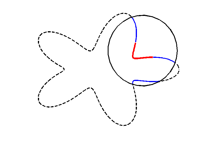
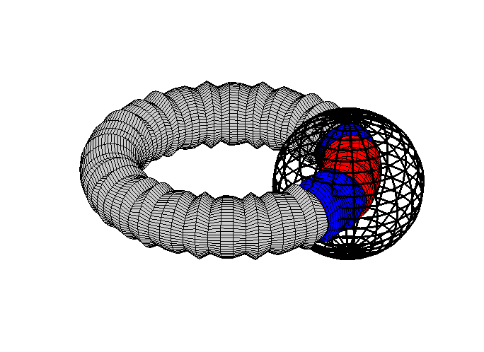
(a)		(b)

Figure 5. Illustration of the geometric objects $\Gamma_{\tau}$, $\Gamma_{\rm near}$ and $\Gamma_{\rm proxy}$ used for the Green’s representation technique for a two-dimensional (a) and three-dimensional surface (b). $\Gamma_{\tau}$ is given in red, $\Gamma_{\rm near}$ is given in blue, and $\Gamma_{\rm proxy}$ is given in black.

5.5.3. The Green’s representation technique

The compression technique described in Section 5.5.2 would be prohibitively expensive if executed as stated, since it requires the formation and factorization of very large matrices. For instance, equation (5.44) requires the factorization of a matrix of size $n_{\tau}\times(N+N_{\rm in}1-n_{\tau})$. It turns out that these computations can be localized by exploiting that the column space of the matrix $\mathsf{B}(I_{\tau},I_{\tau}^{\rm c})$ (which is what we need to span) expresses merely a set of solutions to the homogeneous Helmholtz equation. This means that we can use representation techniques from potential theory to replace all “far-field” interactions by interactions with a small proxy surface $\Gamma_{\rm proxy}$ that encloses the patch $\Gamma_{\tau}$ that we seek to compress. All discretization points inside on $\Gamma_{\rm proxy}$ but not in $\Gamma_{\tau}$ are labeled $\Gamma_{\rm near}$. Figure 5 illustrates the geometry used in the Green’s representation technique for a two-dimensional contour and a three surface that is defined rigorously in Section 6.2. This technique is described in detail in Section 6.2 of [15]. For the experiments in this paper, it is sufficient to let $\Gamma_{\rm proxy}$ be a sphere with a radius that is twice the radius of the smallest ball containing $\Gamma_{\tau}$. (In other words, $\Gamma_{\rm proxy}$ is the surface of the ball “$2B$” defined in Section 3.3.)

6. Numerical experiments.

We now present the results of a number of experiments conducted to measure the performance of the approach of this paper. All code was written in Fortran 77 and compiled with the Intel Fortran Compiler version 12.1. The experiments were carried out on a workstation equipped with $12$ Intel Xeon processor cores running at $3.47$ GHz and $192$ GB of RAM. As a point of reference, we note that MATLAB requires approximately 35 seconds to invert a $8192\times 8192$ matrix with complex-valued i.i.d. Gaussian entries on this workstation.

6.1. Sound-soft scattering from grids of ellipsoids

The purpose of this first set of experiments was to measure the growth in the running time of the algorithm of Section 4 as the geometry of the scatterer becomes more complicated and more nodes are required to discretize it. To that end we considered the exterior Dirichlet problem (DBVP) on a collection of domains consisting of grids of ellipsoids of various sizes and eccentricities. In each experiment, the ellipsoids were arranged on an $n\times n\times n$ grid with center points

$$(1.25+2.5i,1.25+2.5j,1.25+2.5k),\qquad 1\leq i,j,k\leq n.$$

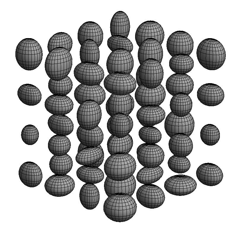
Figure 6. Two views of one of the “grid of ellipsoids” domains of Section 6.1. Domains of this type pose significant challenges for iterative solvers.

Grid dimensions	$N$	$N_{\mbox{\tiny out}}\times N_{\mbox{\tiny in}}$	$T$	$E$	Ratio	Predicted
$2\times 2\times 2$	$12\,288$	$410\times 401$	$1.02\times 10^{+1}$	$3.37\times 10^{-04}$	-	-
$3\times 3\times 3$	$41\,472$	$464\times 475$	$3.43\times 10^{+1}$	$4.81\times 10^{-04}$	3.4	6.2
$4\times 4\times 4$	$98\,304$	$483\times 532$	$7.92\times 10^{+1}$	$1.57\times 10^{-04}$	2.3	3.7
$6\times 6\times 6$	$331\,776$	$504\times 707$	$2.96\times 10^{+2}$	$7.03\times 10^{-04}$	3.7	6.2
$8\times 8\times 8$	$786\,432$	$513\times 1014$	$6.70\times 10^{+2}$	$4.70\times 10^{-04}$	2.3	3.7
$10\times 10\times 10$	$1\,536\,000$	$518\times 1502$	$2.46\times 10^{+3}$	$3.53\times 10^{-04}$	3.7	2.7

Table 2. Results for the experiments of Section 6.1 in the case $\epsilon=1.0\times 10^{-3}$.

The axis lengths of the ellipsoids were determined randomly — each axis length was taken to be $0.5+0.5\eta$ where $\eta$ is a computer-generated pseudorandom number between $0$ and $1$. A $4\times 4\times 4$ domain of this type is depicted in Figure 6. For each experiment, the wavenumber $\kappa$ was chosen to be

$$\kappa=\frac{8\pi}{2.5\times n}$$

so that each domain considered was bounded by a box whose sides were 4 wavelengths in size.

Each experiment consisted of forming a scattering matrix for the integral equation (2.3) and using it to solve an instance of the boundary value problem (DBVP). The boundary data for each problem was taken to be the restriction of the function

$$g(x)=\sum_{j=1}^{N}\frac{\exp(i\kappa|x-x_{j}|)}{|x-x_{j}|},$$

where $N$ is the total number of ellipsoids and the $x_{1},\ldots,x_{N}$ are the centers of the ellipsoids, to the boundary of the ellipsoids. Let $r$ and $x_{0}$ denote the radius and center of the minimum bounding sphere containing the boundary of the domain, respectively. Then the surface $\Gamma_{\mbox{\tiny in}}$ which specified incoming potentials was the union of the spheres of radius $0.1$ centered at the points $x_{1},\ldots,x_{N}$ and the sphere of radius $2r$ centered at $x_{0}$ while the surface $\Gamma_{\mbox{\tiny out}}$ specifying outgoing potentials was taken to be the sphere of radius $2r$ centered at $x_{0}$. The function $g(x)$ is, of course, the unique solution of the boundary value problem and we measured the accuracy of each obtained solution $\sigma$ of the the integral equation by computing the relative error

$$E=\left(\int\hskip-7.0pt\int_{\Gamma}\left|g(x)\right|^{2}dx\right)^{-1/2}\left(\int\hskip-7.0pt\int_{\Gamma}\left|g(x)-(S_{\kappa}+i\kappa D_{\kappa})\sigma(x)\right|^{2}dx\right)^{1/2},$$ (6.1)

where $\Gamma$ is the sphere of radius $2$ centered at the point $x_{0}-(0,0,-2r-10)$. The ellipsoids were parameterized by projection onto the cube $[-1,1]^{3}$ and the faces of the cube were triangulated in order to produce a discretization. Three sets of experiments were performed, each at a different level of desired precision and the ellipsoids were discretized as follows in each case:

1. For precision $\epsilon=1.0\times 10^{-3}$, each cube face comprising the parameterization domain was divided into $8$ triangles and a $32$ point $6$th order quadrature was applied to each triangle. This yields a total of $1536$ discretization nodes per ellipsoid.

2. For precision $\epsilon=1.0\times 10^{-6}$, each cube face was subdivided into $32$ triangles and a $32$ point $6$th order quadrature was applied to each triangle. This resulted in $6144$ discretization nodes per ellipsoid.

3. For precision $\epsilon=1.0\times 10^{-9}$, each cube face was subdivided into $8$ triangles and a $112$ point $12$th order quadrature was applied to each triangle. This results in $5376$ discretization nodes per ellipsoid.

Grid dimensions	$N$	$N_{\mbox{\tiny out}}\times N_{\mbox{\tiny in}}$	$T$	$E$	Ratio	Predicted
$2\times 2\times 2$	$49\,152$	$601\times 584$	$1.61\times 10^{+2}$	$1.22\times 10^{-07}$	-	-
$3\times 3\times 3$	$165\,888$	$676\times 677$	$6.87\times 10^{+2}$	$4.92\times 10^{-07}$	4.3	6.2
$4\times 4\times 4$	$393\,216$	$703\times 747$	$1.68\times 10^{+3}$	$5.31\times 10^{-07}$	2.4	3.6
$6\times 6\times 6$	$1\,327\,104$	$728\times 925$	$6.66\times 10^{+3}$	$4.60\times 10^{-06}$	4.0	6.2
$8\times 8\times 8$	$3\,145\,728$	$742\times 1\,237$	$1.59\times 10^{+4}$	$2.30\times 10^{-07}$	2.4	3.6

Table 3. Results for the numerical experiments of Section 6.1 in the case $\epsilon=1.0\times 10^{-6}.$

Tables 2, 3, and 4 present the results of the experiments with $\epsilon=1.0\times 10^{-3},\,1.0\times 10^{-6},\,1.0\times 10^{-9}$, respectively. In each of those tables, $N$ refers to the number of discretization nodes on the surface; $N_{\mbox{\tiny out}}\times N_{\mbox{\tiny in}}$ denotes the dimension of the resulting scattering matrix; $T$ is the time in seconds required to construct the scattering matrix; $E$ is the error (6.1); Ratio refers to the ratio of running times; and Predicted is the ratio of running times one would expect for an algorithm whose cost scales as $N^{1.5}$.

Grid dimensions	$N$	$N_{\mbox{\tiny out}}\times N_{\mbox{\tiny in}}$	$T$	$E$	Ratio	Predicted
$2\times 2\times 2$	$43\,008$	$997\times 946$	$5.14\times 10^{+2}$	$8.98\times 10^{-09}$	-	-
$3\times 3\times 3$	$145\,152$	$1\,363\times 1\,301$	$2.32\times 10^{+3}$	$4.97\times 10^{-10}$	4.5	6.2
$4\times 4\times 4$	$344\,064$	$1\,377\times 1\,353$	$5.56\times 10^{+3}$	$1.10\times 10^{-10}$	2.4	3.6

Table 4. Results for the numerical experiments of Section 6.1 in the case $\epsilon=1.0\times 10^{-9}.$

Remark 6.1.

The boundary value problems solved in the experiments of this section present considerable difficulties for iterative solvers. We attempted to compare the running time of the fast solver of this paper with the running time of an iterative solver. However, it took more than $1000$ iterations for GMRES residuals to fall below $1.0\times 10^{-3}$ when we attempted to solve the boundary value problem (DBVP) given on the $2\times 2\times 2$ grid of ellipsoids with $1536$ discretization nodes per ellipsoid via the combined field integral equation. Even with the aid of an extremely efficient multipole code, replicating the experiments of this section with an iterative solver appears to be prohibitively expensive.

6.2. Sound-hard scattering from a deformed torus.

In the experiments described here we considered the problem (NBVP) with $\Gamma$ the surface parameterized via

$$\begin{split}r(s,t)=\left(\begin{array}[]{c}(2+0.50\cos(s))\sin(t)\\ (2+0.50\cos(s))\cos(t)\\ 0.50\sin(s)\left(1+0.15\cos(36t)\right)\end{array}\right),\end{split}\ \ \ \ \ \ 0\leq s,t<2\pi.\ \ \$$ (6.2)

Three views of this surface, which is enclosed in the box with lower left corner $(-2.5,-2.5,-0.65)$ and upper right corner $(2.5,2.5,0.65)$, are shown in Figure 7.

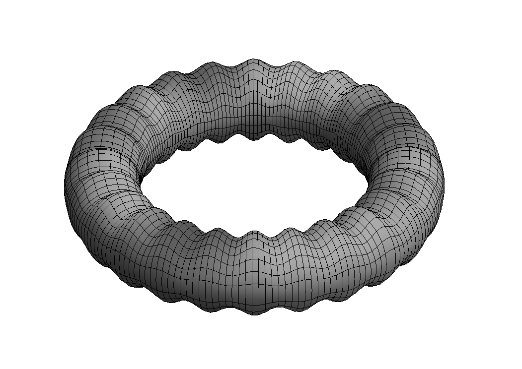
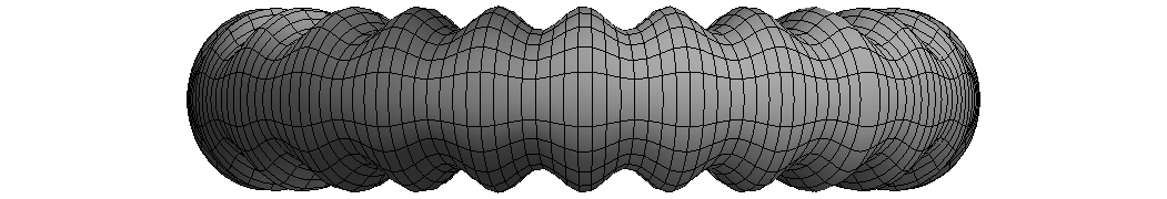
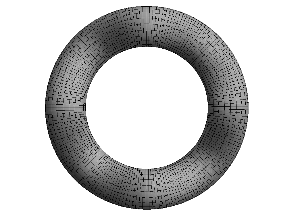
Figure 7. Three views of the deformed torus of Section 6.2.

Each experiment consisted of constructing a scattering matrix for the integral equation formulation (2.4) of the problem (NBVP) and using that scattering matrix to solve an instance of the boundary value problem. The wavenumber $\kappa$ was set at $4\pi/5$, which makes the domain approximately $2\times 2\times 0.7$ wavelengths in size, and the boundary data was taken to be the normal derivative of the function

$$g(x)=\frac{1}{4\pi}\frac{\exp\left(i\kappa\left|x-x_{0}\right|\right)}{\left|x-x_{0}\right|},$$

where $x_{0}$ is the point $(2,0,0)$. Since $x_{0}$ lies inside of the domain $\Omega$, the function $g(x)$ is, of course, the unique solution of (NBVP). The surface $\Gamma_{\mbox{\tiny in}}$ which specified incoming potentials was take to be the union of the sphere of radius $0.1$ centered at the point $(2,0,0)$ and the sphere of radius $6$ centered at $(0,0,0)$ while the surface $\Gamma_{\mbox{\tiny out}}$ specifying outgoing potentials was taken to be the sphere of radius $6$ centered at $(0,0,0)$. The accuracy of each obtained solution $\sigma$ was measured by computing the relative error

$$E=\left(\int\hskip-7.0pt\int_{S}\left|g(x)\right|^{2}dx\right)^{-1/2}\left(\int\hskip-7.0pt\int_{S}\left|g(x)-S_{\kappa}\sigma(x)\right|^{2}dx\right)^{1/2},$$ (6.3)

where $S$ is the sphere of radius $1$ centered at the point $(-20,0,0)$. The order of the discretization quadrature was fixed at $8$ and the requested precision for the scattering matrix was set to $\epsilon=1.0\times 10^{-7}$ in each experiment. The number of triangles used to decompose the parameterization domain was varied.

$N_{\mbox{\tiny tris}}$	$N$	$T$	$E$	$N_{\mbox{\tiny out}}\times N_{\mbox{\tiny in}}$	Ratio	Predicted
$32$	$1\,664$	$7.16\times 10^{+00}$	$3.51\times 10^{-02}$	$395\times 447$	-	-
$128$	$6\,656$	$6.29\times 10^{+01}$	$4.41\times 10^{-03}$	$407\times 460$	$8.79$	$8$
$512$	$26\,624$	$2.81\times 10^{+02}$	$4.08\times 10^{-05}$	$400\times 456$	$4.47$	$8$
$2\,048$	$106\,496$	$2.60\times 10^{+03}$	$7.80\times 10^{-07}$	$408\times 463$	$9.25$	$8$
$8\,192$	$425\,984$	$1.47\times 10^{+04}$	$3.25\times 10^{-08}$	$409\times 466$	$5.66$	$8$

Table 5. The results of the experiments of Section 6.2.

Table 5 shows the results. There, $N_{\mbox{\tiny tris}}$ is the number of triangles into which the parameterization domain was partitioned; $N$ is the total number of discretization nodes on the boundary $\Gamma$; $T$ is the total running time of the algorithm in seconds; $E$ is the relative error (6.3); $N_{\mbox{\tiny out}}\times N_{\mbox{\tiny in}}$ gives the dimensions of the scattering matrix; Ratio is the quotient of the running time at the current level of discretization to the runnning time at the preceeding level of discretization (where it is defined); and Predicted gives the expected ratio of the running times (assuming $O(N^{1.5})$ asymptotic cost).

6.3. A heart-shaped domain.

In these experiments, we solved the problem (NBVP) on the domain $\Omega$ shown in Figure 8. The boundary $\Gamma$ is described by the parameterization

$$r(s,t)=\left(\begin{array}[]{c}\cos(s)\cos(t)+\cos^{2}(s)\sin^{2}(t)\\ \cos(s)\sin(t)\\ \sin(s)\end{array}\right),\ \ \ 0\leq s,t<2\pi,$$

although for the purposes of producing discretizations of the surface $\Gamma$ a parameterization obtained via projection onto a cube was used rather than this function $r(s,t)$. The domain $\Omega$ is contained in the box with lower left corner $(-1,-1,-1)$ and upper right corner $(1.25,1,1)$.

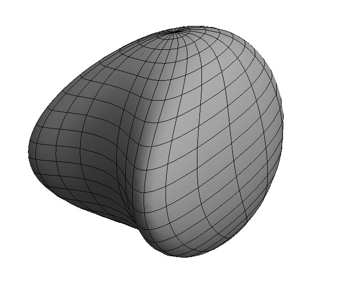
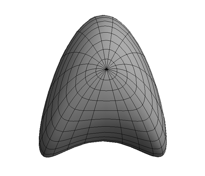
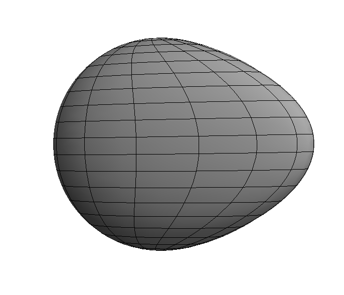
Figure 8. Three views of the heart shaped surface of Section 6.

These experiments consisted of solving the problem (NBVP) on the domain $\Omega$ at a variety of wavenumbers. In each experiment, a scattering matrix for the domain was formed and an instance of the boundary value problem was solved using this scattering matrix. The boundary data was taken to be the derivative of the restriction of the function

$$g(x)=\frac{1}{4\pi}\frac{\exp(i\kappa|x|)}{|x|}$$

to $\Gamma$ with respect to the outward pointing unit normal vector on $\Gamma$. The error in the obtained charge distribution was measured by computing

$$E=\left(\int\hskip-7.0pt\int_{S}\left|g(x)\right|^{2}dx\right)^{-1/2}\left(\int\hskip-7.0pt\int_{S}\left|g(x)-S_{\kappa}\sigma(x)\right|^{2}dx\right)^{1/2},$$ (6.4)

where $S$ is the ball of radius $10$ centered at the point $(-30,-30,-30)$ and $\sigma$ is the approximate charge distribution obtained using the scattering matrix. Discretizations of $\Gamma$ were obtained by triangulating the faces of the cube which constitutes the parameterization domain. An $8$th order discretization quadrature with $45$ points was applied to each triangle. The number of triangles was increased with wavenumber. In all cases, the desired precision for the scattering matrix was taken to be $\epsilon=1.0\times 10^{-3}$. Table 6 reports the number of discretization nodes $N$ on the surface; the relative error $E$; the number of triangles $N_{\rm tris}$ into which the parameterization domain was divided; the total running time $T$; the dimensions $N_{\mbox{\tiny out}}\times N_{\mbox{\tiny in}}$ of the scattering matrix; the wavenumber $\kappa$ for the problem; and the approximate diameter of the domain in wavelengths.

$\kappa$	Diameter	$N_{\mbox{\tiny tris}}$	$N$	$E$	$T$	$N_{\mbox{\tiny out}}\times N_{\mbox{\tiny in}}$
$2\pi$	$3.46\lambda$	$48$	$2\,496$	$4.20\times 10^{-04}$	$6.84\times 10^{+00}$	$251\times 229$
$4\pi$	$6.92\lambda$	$192$	$9\,984$	$1.33\times 10^{-04}$	$6.93\times 10^{+01}$	$571\times 546$
$6\pi$	$10.39\lambda$	$768$	$39\,936$	$1.88\times 10^{-04}$	$3.74\times 10^{+02}$	$996\times 972$
$8\pi$	$13.87\lambda$	$768$	$39\,936$	$3.61\times 10^{-04}$	$4.99\times 10^{+02}$	$1491\times 1\,471$
$10\pi$	$17.32\lambda$	$3\,072$	$159\,744$	$4.96\times 10^{-04}$	$2.83\times 10^{+03}$	$2157\times 2\,126$
$12\pi$	$20.79\lambda$	$3\,072$	$159\,744$	$1.89\times 10^{-04}$	$3.78\times 10^{+03}$	$2851\times 2\,829$
$14\pi$	$24.25\lambda$	$12\,288$	$638\,976$	$6.75\times 10^{-04}$	$1.81\times 10^{+04}$	$3615\times 3\,589$

Table 6. The results of the experiments of Section 6.

6.4. Scattering from a deformed cube.

In this next set of experiments, we considered the problem (NBVP) on a deformed cube $\Omega$ with $12$ curved edges and $8$ corner points. The domain $\Omega$ is pictured in Figure 9. The top face of the boundary $\Gamma$ was parameterized over the region $-1\leq s,t\leq 1$ via

$$r(s,t)=\left(2+s^{2}+t^{2}\right)\left(\begin{array}[]{c}s\\ t\\ 1\end{array}\right)$$

and the other faces were handled in a like manner. The domain $\Omega$ is contained in the box with lower left corner $(-4,-4,-4)$ and upper right corner $(4,4,4)$.

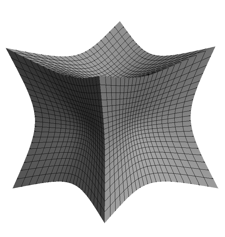
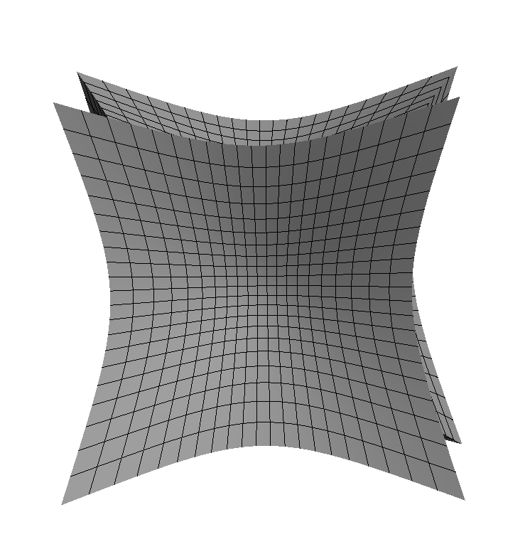
Figure 9. The deformed cube domain considered in Section 7. The domain has $12$ curved edges and $8$ corner points.

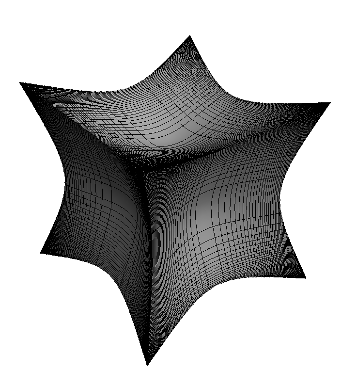
Figure 10. Illustration of the unevenly refined grid used to generate discretization nodes on the deformed cube surface considered in Section 7.

In these experiments, the integral equation (2.4) defined on $\Gamma$ was discretized by applying a $12$th order discretization quadrature with $112$ nodes to increasing dense triangulations of the parameterization domain. We arranged for a denser distribution of discretization nodes near the edges and corners of the deformed cube. Figure 10 shows one of the unevenly refined meshes used in these experiments.

A scattering matrix was constructed for each discretization and an instance of the boundary value problem was solved using this scattering matrix. In each experiment, the wavenumber was taken to be $\kappa=\pi/2$, making the domain roughly $3.46$ wavelengths in diameter, the desired precision for the scattering matrix was set to $\epsilon=1.0\times 10^{-10}$ and the boundary data was taken to be the outward normal derivative on $\Gamma$ of the function

$$g(x)=\frac{1}{4\pi}\int\hskip-7.0pt\int_{\Gamma_{\mbox{\tiny in}}}\frac{\exp(i\kappa|x-y|)}{|x-y|}ds(y),$$

where $\Gamma_{\mbox{\tiny in}}$ denotes the sphere of radius $0.1$ centered at the point $(0.1,0,0)$. The error in the obtained charge distribution $\sigma$ was measured via the quantity

$$E=\left(\int\hskip-7.0pt\int_{\Gamma_{\mbox{\tiny out}}}\left|g(x)\right|^{2}dx\right)^{-1/2}\left(\int\hskip-7.0pt\int_{\Gamma_{\mbox{\tiny out}}}\left|g(x)-S_{\kappa}\sigma(x)\right|^{2}dx\right)^{1/2},$$ (6.5)

where $\sigma$ is the obtained charge distribution and ${\Gamma_{\mbox{\tiny out}}}$ denotes the sphere of radius $1$ centered at the point $(-10,-10,0)$. Table 7 reports the error (6.5) along with $N_{\rm tris}$, $N$, $T$ and $N_{\mbox{\tiny out}}\times N_{\mbox{\tiny in}}$ (whose meanings are as in the preceding sections).

$N_{\mbox{\tiny tris}}$	$N$	$E$	$T$	$N_{\mbox{\tiny out}}\times N_{\mbox{\tiny in}}$
$192$	$21\,504$	$2.60\times 10^{-08}$	$6.11\times 10^{+02}$	$617\times 712$
$432$	$48\,384$	$2.13\times 10^{-09}$	$1.65\times 10^{+03}$	$620\times 694$
$768$	$86\,016$	$3.13\times 10^{-10}$	$3.58\times 10^{+03}$	$612\times 685$

Table 7. The results of the experiments preformed on the deformed cube of Section 7.

6.5. A Convergence Study involving a Trefoil Domain

The experiments described in the preceding sections all involved problems with artifical boundary data associated with known solutions. In this section, we describe an experiment for which we did not have access to an exact solution, and instead estimate the error by comparing against a very finely resolved computed solution.

We considered the boundary value problem (DBVP) given on the trefoil domain $\Omega$ shown in Figure 11. The parameterization of the boundary of $\Omega$ is given by

$$r(s,t)=\bm{\gamma}(s)+\cos(s)\bm{n}(s)+\sin(-t)\bm{b}(s),\ \ \ 0\leq s,t<2\pi,$$

where

$$\bm{\gamma}(s)=\left(\begin{array}[]{c}\sin(3s)\\ \sin(s)+2\sin(2s)\\ \cos(s)-2\cos(s)\end{array}\right),$$

$\bm{n}(s)$ is the unit normal vector to the curve $\gamma(s)$ at $s$ and $\bm{b}(s)$ is the unit binormal vector at $s$. The domain is contained in a box with bottom left corner at $[-1.5,-3,-3.5]$ and top right corner $[1.5,3,3.5]$.

Discretizations of the surface $\Gamma$ were formed by partitioning the parameter space into $N_{\rm tris}$ triangles and utilizing an $8$th order (52 point) quadrature on each triangle so that $N=52N_{\rm tris}$. A scattering matrix for each discretization was then formed; $\Gamma_{\rm in}$ consisted of the point $(1,0,0)$ and $\Gamma_{\rm out}$ was taken to be the surface of a sphere of radius $1$ centered at $(30,30,30)$. The boundary data was generated by a point charge on $\Gamma_{\rm in}$. As the solution to this problem is unknown, we report the $L^{2}$ convergence of the solution on the surface of $\Gamma_{\rm out}$. Specifically, we report

$$E_{N}=\left(\int\hskip-7.0pt\int_{\Gamma_{\rm out}}\left|(S_{\kappa}+i\kappa D_{\kappa})\sigma_{4N}(x)-(S_{\kappa}+i\kappa D_{\kappa})\sigma_{N}(x)\right|^{2}dx\right)^{1/2},$$ (6.6)

where $\sigma_{N}$ is the computed boundary charge distribution with $N$ discretization points.

We considered two choices of wavenumber and tolerance: (i) the domain was approximately $1\times 3\times 3$ wavelengths in size and the tolerance is set to $\epsilon=10^{-9}$; (ii) the domain was approximately $2\times 6\times 6$ wavelengths in size and the tolerance is set to $\epsilon=10^{-6}$. Tables 8 and 9 report on the convergence of the solution as the number of discretization points $N$ is increased.

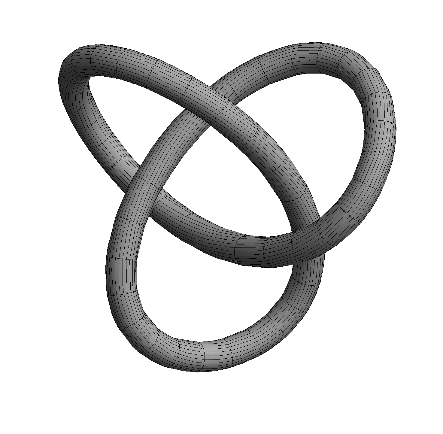
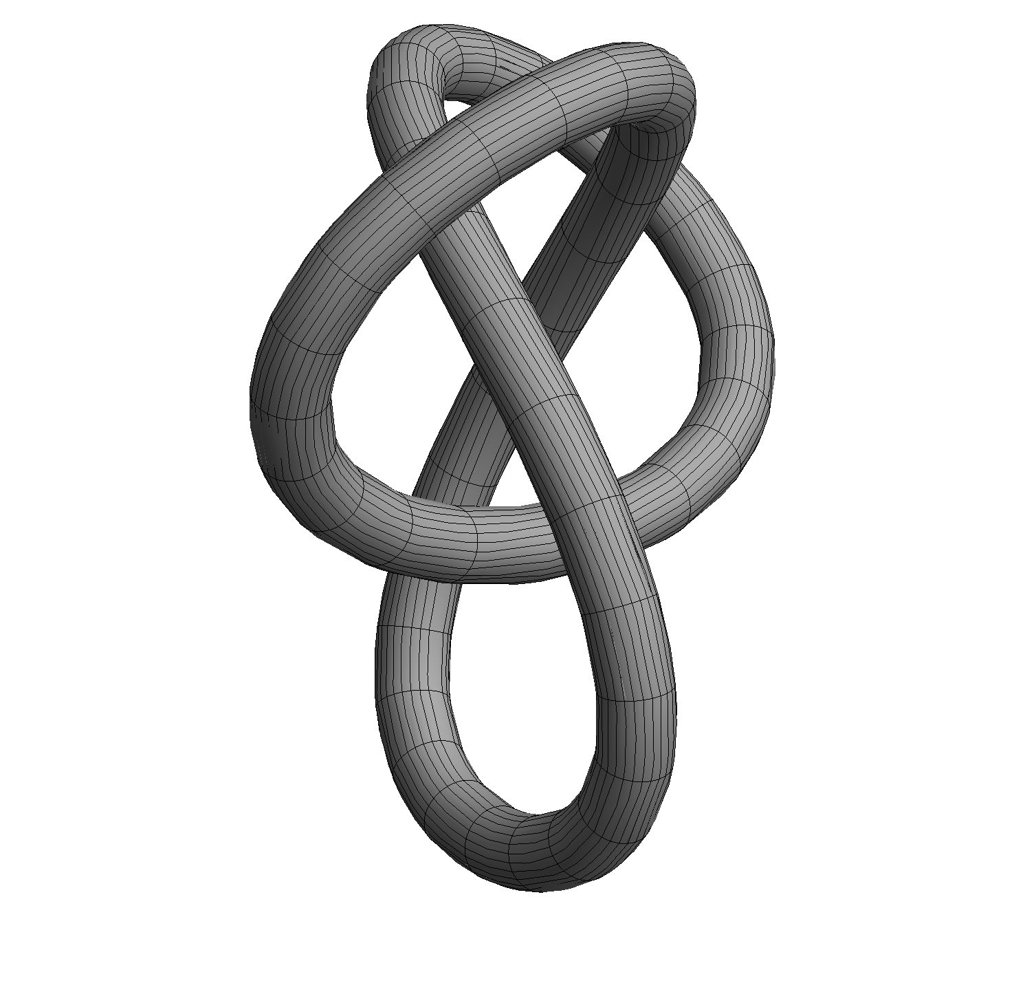
Figure 11. The trefoil domain $\Omega$ considered in Section 9.

$N_{\mbox{\tiny tris}}$	$N$	$E_{N}$	$T$	$N_{\mbox{\tiny out}}\times N_{\mbox{\tiny in}}$
$16$	$832$	$6.73\times 10^{-04}$	$1.17\times 10^{+00}$	$754\times 737$
$64$	$3\,328$	$2.33\times 10^{-06}$	$3.78\times 10^{+01}$	$939\times 910$
$256$	$13\,312$	$2.59\times 10^{-08}$	$3.61\times 10^{+02}$	$945\times 917$
$1\,024$	$53\,248$	$2.47\times 10^{-11}$	$2.55\times 10^{+03}$	$948\times 918$
$4\,096$	$212\,992$	-	$2.83\times 10^{+04}$	$949\times 921$

Table 8. The results for the experiments performed on the trefoil of Section 9 when the domain is is approximately $1\times 3\times 3$ wavelengths in size and $\epsilon=10^{-9}$.

$N_{\mbox{\tiny tris}}$	$N$	$E_{N}$	$T$	$N_{\mbox{\tiny out}}\times N_{\mbox{\tiny in}}$
$16$	$832$	$2.87\times 10^{-02}$	$1.94\times 10^{+00}$	$832\times 832$
$64$	$3\,328$	$1.08\times 10^{-03}$	$7.59\times 10^{+01}$	$1\,771\times 1\,745$
$256$	$13\,312$	$5.57\times 10^{-06}$	$4.12\times 10^{+02}$	$1\,820\times 1\,782$
$1\,024$	$53\,248$	$3.04\times 10^{-08}$	$2.16\times 10^{+03}$	$1\,822\times 1\,788$
$4\,096$	$212\,992$	-	$1.27\times 10^{+04}$	$1\,828\times 1\,794$

Table 9. The results for the experiments performed on the trefoil of Section 9 when the domain is is approximately $2\times 6\times 6$ wavelengths in size and $\epsilon=10^{-6}$.

7. Acknowledgements

J. Bremer was supported by a fellowship from the Alfred P. Sloan Foundation and by the Office of Naval Research under contract N00014-12-1-0117. P.G. Martinsson was supported by the National Science Foundation under contracts DMS0748488 and DMS0941476.

Appendix A A robust integral formulation for solving (NBVP)

Consider the task of solving the Neumann boundary value problem (NBVP) using a boundary integral equation formulation. In order to avoid the problem of spurious resonances, it would be natural to use a combined layer representation of the form

$$u(x)=D_{\kappa}\sigma(x)+i|\kappa|S_{\kappa}\sigma(x).$$ (A.1)

However, the BIE obtained by simply combining (A.1) with the Neumann boundary condition involves the hypersingular operator

$$N_{\kappa}\sigma(x)=\int_{\partial\Omega}\left(\eta_{x}\cdot\nabla_{x}\left(\eta_{y}\cdot\nabla_{y}G_{\kappa}(x,y)\right)\right)\sigma(y)ds(y).$$

Two difficulties are encountered when handling integral equations involving hypersingular operators:

1. Viewed as an operator from $L^{2}(\Gamma)$ to $L^{2}(\Gamma)$, $N_{\kappa}$ is not bounded. In consequence, if standard discretization methods are applied to integral equations involving this operator, ill-conditioned linear systems will result. This complication can be overcome by viewing $N_{\kappa}$ as on operator between two different Sobolev spaces; however, more complicated analytic machinery would then be required.

2. The singularity in the kernel of the hypersingular operator $N_{\kappa}$ is more severe than the singularities of the standard operators of acoustic scattering. As discussed in [8], the approach used here to evaluate singular integrals can be generalized to this case. However, considerable work is required and the resulting quadratures are somewhat less efficient than those used here.

A technique known as “regularization” offers an alternative to handling the operator $N_{\kappa}$ [11]. For example, the representation (2.2) can be replaced with

$$u(x)=S_{\kappa}\sigma(x)+D_{\kappa}S_{\kappa}\sigma(x)$$

which leads to the integral equation

$$-\frac{1}{2}\sigma(x)+[N_{\kappa}S_{\kappa}]\sigma(x)+D_{\kappa}^{*}\sigma(x)=g(x).$$ (A.2)

Using Calderón identities (which are discussed in, for instance, [28]), we can rewrite (A.2) as

$$-\frac{3}{4}\sigma(x)+D_{\kappa}^{*}\sigma(x)+(D_{\kappa}^{*})^{2}\sigma(x)=g(x),$$ (A.3)

which does not involve hypersingular operators. While the equation (A.3) is suitable for use by iterative solvers, the composition of the operator $D_{\kappa}^{*}$ makes it cumbersome for direct solvers.

To make the formulation (A.3) more suitable for direct solvers, we introduce an auxiliary variable

$$\phi(x)=D_{\kappa}^{*}\sigma(x),$$

which results to the system of integral equations

$$\begin{split}-\frac{3}{4}\sigma(x)+D_{\kappa}^{*}\sigma(x)+D_{\kappa}^{*}\phi(x)&=g(x)\\ -\phi(x)+D_{\kappa}^{*}\sigma(x)&=0.\end{split}$$ (A.4)

The system (A.4) is now ideal for direct solvers as it does not involve hypersingular operators and no compositions of operators appear.

Appendix B Derivation of scattering matrices and the merge formula from a field formulation

The derivation of the formula for merging two scattering matrices given in Section 5.4 is quite formal. In this section, we provide a different derivation that is hopefully more intuitive and gives a better idea of the physical meaning of a scattering matrix $\mathsf{S}_{\tau}$ for a subpatch $\Gamma_{\tau}\subseteq\Gamma$. This derivation was omitted from the main text since it requires the introduction of several auxiliary fields.

Throughout this section of the appendix, we rely on the hierarchical tree partitioning of the domain $\Gamma$ described in Section 5.2, and the associated HBS representation of a matrix given in Section 5.3.

B.1. Problem formulation

Our objective is to evaluate the map (4.4), which is the discretization of the scattering problem (4.1). We restate it for easy reference: Given a vector $\bm{s}_{\rm in}$ representing a source distribution on the “radiation source,” we seek to compute the field $\bm{u}_{\rm out}$ on the “antenna” given by

$$\begin{array}[]{ccccccccc}\bm{u}_{\rm out}&=&\mathsf{A}_{\rm out}&\mathsf{A}^{-1}&\mathsf{A}_{\rm in}&\bm{s}_{\rm in},\\[5.69054pt] N_{\rm out}\times 1&&N_{\rm out}\times N&N\times N&N\times N_{\rm in}&N_{\rm in}\times 1\end{array}$$ (B.1)

We define the external incoming field on the scattering surface $\Gamma$ via

$$\bm{u}=\mathsf{A}_{\rm in}\bm{s}_{\rm in}.$$

The core task is then to solve the equation

$$\mathsf{A}\bm{\sigma}=\bm{u}$$ (B.2)

to compute the field of induced charges $\bm{\sigma}$ on $\Gamma$. As described in Section 4.2, we do not need to solve (B.2) in full generality, but only under two simplifying constraints:

1. The external incoming field $\bm{u}$ is restricted to a low-dimensional space spanned by the provided basis matrix $\hat{\mathsf{U}}_{1}$. In other words, there exists a short vector $\tilde{\bm{u}}_{1}$ such that $\bm{u}=\hat{\mathsf{U}}_{1}\,\tilde{\bm{u}}_{1}$.

2. We only need the projection of $\bm{\sigma}$ onto a low-dimensional space spanned by the provided basis matrix $\hat{\mathsf{V}}_{1}$. In other words, we only need the short vector $\tilde{\bm{\sigma}}_{1}=\hat{\mathsf{V}}_{1}^{*}\bm{\sigma}$.

For convenience in the hierarchical formulation of the scattering problem, we define for a subpatch $\Gamma_{\tau}$ of the scattering surface an internal incoming field via

$$\bm{v}_{\tau}=\mathsf{A}(I_{\tau},I_{\tau}^{\rm c})\,\bm{\sigma}(I_{\tau}^{\rm c}).$$ (B.3)

Then $\bm{v}_{\tau}$ is the field on $\Gamma_{\tau}$ induced by charges on $\Gamma\backslash\Gamma_{\tau}$. For a node $\tau$, the restriction of (B.2) to $I_{\tau}$,

$$\mathsf{A}(I_{\tau},I_{\tau})\,\bm{\sigma}(I_{\tau})+\mathsf{A}(I_{\tau},I_{\tau}^{\rm c})\,\bm{\sigma}(I_{\tau}^{\rm c})=\bm{u}(I_{\tau})$$ (B.4)

can then be written

$$\mathsf{A}(I_{\tau},I_{\tau})\,\bm{\sigma}(I_{\tau})=\bm{u}(I_{\tau})-\bm{v}_{\tau}.$$ (B.5)

In words, equation (B.5) states that the induced charges $\bm{\sigma}(I_{\tau})$ on $\Gamma_{\tau}$ must create a local field that precisely match the total incoming field $\bm{u}(I_{\tau})-\bm{v}_{\tau}$, which is the difference between the externally imposed incoming field $\bm{u}(I_{\tau})$ and the internal incoming field $\bm{v}_{\tau}$ which is caused by induced charges on the rest of $\Gamma$.

B.2. Short representations and the definition of the scattering matrix

By definition, the columns of the long basis matrix $\hat{\mathsf{U}}_{\tau}$ span both the restriction $\bm{u}(I_{\tau})$ of the external incoming field to the patch $\Gamma_{\tau}$, and the columns of the off-diagonal block $\mathsf{A}(I_{\tau},I_{\tau}^{\rm c})$. As a consequence, there exist short vectors $\tilde{\bm{u}}_{\tau}$ and $\tilde{\bm{v}}_{\tau}$ such that

$$\bm{v}_{\tau}=\hat{\mathsf{U}}_{\tau}\,\tilde{\bm{v}}_{\tau},\qquad\mbox{and}\qquad\bm{u}(I_{\tau})=\hat{\mathsf{U}}_{\tau}\,\tilde{\bm{u}}_{\tau}.$$ (B.6)

We say that $\tilde{\bm{v}}_{\tau}$ and $\tilde{\bm{u}}_{\tau}$ are the compressed representations of $\bm{v}_{\tau}$ and $\bm{u}(I_{\tau})$, respectively. Using these representations, (B.5) can be written

$$\mathsf{A}(I_{\tau},I_{\tau})\,\bm{\sigma}(I_{\tau})=\hat{\mathsf{U}}_{\tau}\,\bigl{(}\tilde{\bm{u}}_{\tau}-\tilde{\bm{v}}_{\tau}\bigr{)}.$$ (B.7)

We also define a compressed representation of the induced charges $\bm{\sigma}(I_{\tau})$ on $\Gamma_{\tau}$ via

$$\tilde{\bm{\sigma}}_{\tau}=\hat{\mathsf{V}}_{\tau}^{*}\bm{\sigma}(I_{\tau}).$$ (B.8)

Multiplying (B.7) by $\hat{\mathsf{V}}_{\tau}^{*}\mathsf{A}(I_{\tau},I_{\tau})^{-1}$, we now get the scattering equation

$$\tilde{\bm{\sigma}}_{\tau}=\mathsf{S}_{\tau}\,\bigl{(}\tilde{\bm{u}}_{\tau}-\tilde{\bm{v}}_{\tau}\bigr{)},$$ (B.9)

where, recall from (4.6),

$$\mathsf{S}_{\tau}=\hat{\mathsf{V}}_{\tau}^{*}\mathsf{A}(I_{\tau},I_{\tau})^{-1}\hat{\mathsf{U}}_{\tau}.$$ (B.10)

Equation (B.9) states that the scattering matrix $\mathsf{S}_{\tau}$ maps the short representation $\tilde{\bm{u}}_{\tau}-\tilde{\bm{v}}_{\tau}$ of the total incoming field on $\Gamma_{\tau}$ to the short representation $\tilde{\bm{\sigma}}_{\tau}$ of the induced charges.

B.3. Hierarchical construction of scattering matrices

For leaf nodes $\tau$, we compute $\mathsf{S}_{\tau}$ directly from the definition (B.10). For parent nodes, we compute the scattering matrices via a hierarchical merging procedure; it turns out that if we know the scattering matrices $\mathsf{S}_{\alpha}$ and $\mathsf{S}_{\beta}$ of the children $\{\alpha,\beta\}$ of a node $\tau$, then $\mathsf{S}_{\tau}$ can be built inexpensively as follows: Observe that (B.7) can be written

$$\left[\begin{array}[]{cc}\mathsf{A}(I_{\alpha},I_{\alpha})&\mathsf{A}(I_{\alpha},I_{\beta})\\ \mathsf{A}(I_{\beta},I_{\alpha})&\mathsf{A}(I_{\beta},I_{\beta})\end{array}\right]\left[\begin{array}[]{c}\bm{\sigma}(I_{\alpha})\\ \bm{\sigma}(I_{\beta})\end{array}\right]=\hat{\mathsf{U}}_{\tau}\,\bigl{(}\tilde{\bm{u}}_{\tau}-\tilde{\bm{v}}_{\tau}\bigr{)}.$$ (B.11)

Inserting into (B.11) the factorizations (5.2) of $\mathsf{A}(I_{\alpha},I_{\beta})$ and $\mathsf{A}(I_{\beta},I_{\alpha})$, and the hierarchical representation (5.7) of $\hat{\mathsf{U}}_{\tau}$, we get

$$\left[\begin{array}[]{cc}\mathsf{A}(I_{\alpha},I_{\alpha})&\hat{\mathsf{U}}_{\alpha}\tilde{\mathsf{A}}_{\alpha,\beta}\hat{\mathsf{V}}_{\beta}^{*}\\ \hat{\mathsf{U}}_{\beta}\tilde{\mathsf{A}}_{\beta,\alpha}\hat{\mathsf{V}}_{\alpha}^{*}&\mathsf{A}(I_{\beta},I_{\beta})\end{array}\right]\left[\begin{array}[]{c}\bm{\sigma}(I_{\alpha})\\ \bm{\sigma}(I_{\beta})\end{array}\right]=\left[\begin{array}[]{cc}\hat{\mathsf{U}}_{\alpha}&\mathsf{0}\\ \mathsf{0}&\hat{\mathsf{U}}_{\beta}\end{array}\right]\,\mathsf{U}_{\tau}\,\bigl{(}\tilde{\bm{u}}_{\tau}-\tilde{\bm{v}}_{\tau}\bigr{)}.$$ (B.12)

Left-multiply (B.12) by $\left[\begin{array}[]{cc}\hat{\mathsf{V}}_{\alpha}^{*}\mathsf{A}(I_{\alpha},I_{\alpha})^{-1}&\mathsf{0}\\ \mathsf{0}&\hat{\mathsf{V}}_{\beta}^{*}\mathsf{A}(I_{\beta},I_{\beta})^{-1}\end{array}\right]$ to obtain

$$\left[\begin{array}[]{cc}\mathsf{I}&\mathsf{S}_{\alpha}\tilde{\mathsf{A}}_{\alpha,\beta}\\ \mathsf{S}_{\beta}\tilde{\mathsf{A}}_{\beta,\alpha}&\mathsf{I}\end{array}\right]\left[\begin{array}[]{c}\tilde{\bm{\sigma}}_{\alpha}\\ \tilde{\bm{\sigma}}_{\beta}\end{array}\right]=\left[\begin{array}[]{cc}\mathsf{S}_{\alpha}&\mathsf{0}\\ \mathsf{0}&\mathsf{S}_{\beta}\end{array}\right]\,\mathsf{U}_{\tau}\,\bigl{(}\tilde{\bm{u}}_{\tau}-\tilde{\bm{v}}_{\tau}\bigr{)}.$$ (B.13)

Solving (B.13) for $\{\tilde{\bm{\sigma}}_{\alpha},\tilde{\bm{\sigma}}_{\beta}\}$ and left multiplying the result by $\mathsf{V}_{\tau}^{*}$, we find

$$\underbrace{\mathsf{V}_{\tau}^{*}\left[\begin{array}[]{c}\tilde{\bm{\sigma}}_{\alpha}\\ \tilde{\bm{\sigma}}_{\beta}\end{array}\right]}_{=\tilde{\bm{\sigma}}_{\tau}}=\underbrace{\mathsf{V}_{\tau}^{*}\left[\begin{array}[]{cc}\mathsf{I}&\mathsf{S}_{\alpha}\tilde{\mathsf{A}}_{\alpha,\beta}\\ \mathsf{S}_{\beta}\tilde{\mathsf{A}}_{\beta,\alpha}&\mathsf{I}\end{array}\right]^{-1}\left[\begin{array}[]{cc}\mathsf{S}_{\alpha}&\mathsf{0}\\ \mathsf{0}&\mathsf{S}_{\beta}\end{array}\right]\,\mathsf{U}_{\tau}}_{=\mathsf{S}_{\tau}}\bigl{(}\tilde{\bm{u}}_{\tau}-\tilde{\bm{v}}_{\tau}\bigr{)}.$$ (B.14)

Comparing equation (B.14) to (B.9), we rediscover the formula (5.16) for the merge of two scattering matrices given in Lemma 5.1.

References

- [1] Barnett, A., and Greengard, L. A new integral representation for quasi-periodic fields and its application to two-dimensional band structure calculations. Journal of Computational Physics 229 (2010), 6898–6914.
- [2] Börm, S. Efficient numerical methods for non-local operators, vol. 14 of EMS Tracts in Mathematics. European Mathematical Society (EMS), Zürich, 2010. -matrix compression, algorithms and analysis.
- [3] Börm, S., and Hackbusch, W. Approximation of boundary element operators by adaptive -matrices. In Foundations of computational mathematics: Minneapolis, 2002, vol. 312 of London Math. Soc. Lecture Note Ser. Cambridge Univ. Press, Cambridge, 2004, pp. 58–75.
- [4] Brakhage, H., and Werner, P. über das dirichletsche ausssenraum problem für die helmholtzsche schwingungsgleihung. Arch. Math 16 (1965), 325–329.
- [5] Bremer, J. A fast direct solver for the integral equations of scattering theory on planar curves with corners. Journal of Computational Physics 231 (2012), 45–64.
- [6] Bremer, J. On the Nyström discretization of integral operators on planar domains with corners. Applied and Computational Harmonic Analysis 32 (2012), 45–64.
- [7] Bremer, J., and Gimbutas, Z. A Nyström method for weakly singular integral operators on surfaces. Journal of Computational Physics 231 (2012), 4885–4903.
- [8] Bremer, J., and Gimbutas, Z. On the numerical evaluation of the singular integrals of scattering theory. Journal of Computational Physics 251 (2013), 327–343.
- [9] Bremer, J., Gimbutas, Z., and Rokhlin, V. A nonlinear optimization procedure for generalized Gaussian quadratures. SIAM Journal of Scientific Computing 32 (2010), 1761–1788.
- [10] Bremer, J., Rokhlin, V., and Sammis, I. Universal quadratures for boundary integral equations on two-dimensional domains with corners. Journal of Computational Physics 229 (2010), 8259–8280.
- [11] Bruno, O., Elling, T., and Turc, C. Well-conditioned high-order algorithms for the solution of three-dimensional surface acoustic scattering problems with Neumann boundary conditions. Journal of Numerical Methods in Engineering 91 (2012), 1045–1072.
- [12] Chandrasekaran, S., and Gu, M. Fast and stable algorithms for banded plus semiseparable systems of linear equations. SIAM J. Matrix Anal. Appl. 25, 2 (2003), 373–384 (electronic).
- [13] Cheng, H., Gimbutas, Z., Martinsson, P., and Rokhlin, V. On the compression of low rank matrices. SIAM Journal of Scientific Computing 26, 4 (2005), 1389–1404.
- [14] Colton, D., and Kress, R. Inverse Acoustic and Electromagnetic Scattering Theory, 2nd ed. Springer-Verlag, New York, 1998.
- [15] Gillman, A., Young, P., and Martinsson, P.-G. A direct solver complexity for integral equations on one-dimensional domains. Frontiers of Mathematics in China 7 (2012), 217–247. 10.1007/s11464-012-0188-3.
- [16] Grasedyck, L., and Hackbusch, W. Construction and arithmetics of -matrices. Computing 70, 4 (2003), 295–334.
- [17] Greengard, L., Gueyffier, D., Martinsson, P.-G., and Rokhlin, V. Fast direct solvers for integral equations in complex three-dimensional domains. Acta Numer. 18 (2009), 243–275.
- [18] Gu, M., and Eisenstat, S. C. Efficient algorithms for computing a strong rank-revealing QR factorization. SIAM J. Sci. Comput. 17, 4 (1996), 848–869.
- [19] Hackbusch, W. Integral Equations: theory and numerical treatment. Birkhäuser, Berlin, 1995.
- [20] Hackbusch, W., Khoromskij, B., and Sauter, S. On -matrices. In Lectures on Applied Mathematics. Springer Berlin, 2002, pp. 9–29.
- [21] Halko, N., Martinsson, P.-G., and Tropp, J. A. Finding structure with randomness: Probabilistic algorithms for constructing approximate matrix decompositions. SIAM Review 53, 2 (2011), 217–288.
- [22] Helsing, J. A fast and stable solver for singular integral equations on piecewise smooth curves. SIAM Journal of Scientific Computing 33 (2011), 153–174.
- [23] Helsing, J., and Ojala, R. Corner singularities for elliptic problems: integral equations, graded meshes, quadrature, and compressed inverse preconditioning. Journal of Computational Physics 227 (2008), 8820–8840.
- [24] Ho, K., and Greengard, L. A fast direct solver for structured linear systems by recursive skeletonization. SIAM Journal on Scientific Computing 34, 5 (2012), 2507–2532.
- [25] Kress, R. Integral Equations. Springer-Verlag, New York, 1999.
- [26] Martinsson, P., and Rokhlin, V. A fast direct solver for boundary integral equations in two dimensions. J. Comp. Phys. 205, 1 (2005), 1–23.
- [27] Martinsson, P., and Rokhlin, V. A fast direct solver for boundary integral equations in two dimensions. Journal of Computational Physics 205 (2006).
- [28] Nédélec, J.-C. Acoustic and Electromagnetic Equations: Integral Representations for Harmonic Functions. Springer, New York, 2012.
- [29] Sheng, Z., Dewilde, P., and Chandrasekaran, S. Algorithms to solve hierarchically semi-separable systems. In System theory, the Schur algorithm and multidimensional analysis, vol. 176 of Oper. Theory Adv. Appl. Birkhäuser, Basel, 2007, pp. 255–294.
- [30] Taskinen, M., and Yla-Oijala, P. Current and charge integral equation formulation. IEEE Transactions on Antennas and Propagation 54 (2006), 58–67.
- [31] Xia, J., Chandrasekaran, S., Gu, M., and Li, X. Fast algorithms for hierarchically semiseparable matrices. Numerical Linear Algebra with Applications 17, 6 (2010), 953–976.
- [32] Xia, J., Chandrasekaran, S., Gu, M., and Li, X. S. Superfast multifrontal method for large structured linear systems of equations. SIAM J. Matrix Anal. Appl. 31, 3 (2009), 1382–1411.
- [33] Xia, J., Chandrasekaran, S., Gu, M., and Li, X. S. Fast algorithms for hierarchically semiseparable matrices. Numerical Linear Algebra with Applications 17, 6 (2010), 953–976.