Lepton flavor-violating transitions in effective field theory and gluonic operators

Abstract

Lepton flavor-violating processes offer interesting possibilities to probe new physics at multi-TeV scale. We discuss those in the framework of effective field theory, emphasizing the role of gluonic operators. Those operators are obtained by integrating out heavy quarks that are kinematically inaccessible at the scale where low-energy experiments take place and make those experiments sensitive to the couplings of lepton flavor changing neutral currents to heavy quarks. We discuss constraints on the Wilson coefficients of those operators from the muon conversion $\mu^{-}+(A,Z)\to e^{-}+(A,Z)$ and from lepton flavor-violating tau decays with one or two hadrons in the final state, e.g. $\tau\to\ell\ \eta^{(\prime)}$ and $\tau\to\ell\ \pi^{+}\pi^{-}$ with $\ell=\mu,e$. To illustrate the results we discuss explicit examples of constraining parameters of leptoquark models.

I Introduction

As follows from observations of neutrino oscillations, there is a good evidence that the individual lepton flavor is not conserved. Explicit calculations of the standard model (SM) rates for the charged lepton-flavor violating (LFV) transitions indicate that those are tiny Marciano:1977wx ; Vergados:1985pq , well beyond the capabilities of current and currently planned experiments. Yet, many models of beyond the standard model (BSM) physics do not exclude relatively large rates for such transitions, so experimental and theoretical studies of LFV processes like $\mu\to e\gamma$, $\tau\to\eta^{(\prime)}\mu$ or $\mu^{-}+(A,Z)\to e^{-}+(A,Z)$ could provide a sensitive test of those BSM schemes.

The language of effective field theory (EFT) is very useful in the studies of flavor violating processes for several reasons. First, it allows to probe the new physics (NP) scale generically, without specifying a particular model of NP. Studies of specific models in this framework are equivalent to specifying Wilson coefficients of effective operators. Second, EFT allows for studies of relative contributions of various operators and may even provide clues as to what experiments need to be done to discriminate among different possible models of new physics Cirigliano:2009bz .

Interactions of flavor-changing neutral currents (FCNC) of leptons with hadrons, either in muon conversion or in tau or meson decays can be described in terms of effective operators of increasing dimension Cirigliano:2009bz . In order to set up an EFT calculation, however, one must first discuss the multitude of scales present in lepton FCNC transitions. The highest scale, which we denote as $\Lambda$, is the scale associated with new physics that generates the FCNC interaction. There could be many ways to generate the flavor-changing neutral current of leptons, yet, below the scale $\Lambda$ any heavy new physics particles are integrated out resulting only in a few effective operators Golowich:2007ka . We shall keep track of the leading contribution due to NP which, below the scale $\Lambda$, is proportional to $1/\Lambda^{2}$. The second highest scale is the one associated with electroweak symmetry breaking, $v$. The most important scales for this study are the scales associated with heavy quark masses, $m_{t}$, $m_{b}$, and $m_{c}$. In the framework of EFT one must integrate out heavy quarks that are not kinematically accessible at the scale where the experiment takes place, resulting in changes of Wilson coefficients of quark and gluon operators.

The relation between all those scales can be done with the help of renormalization group, keeping track of which degrees of freedom are kept and which are integrated out. We shall list the most important operators for our analysis below.

I.1 Quark operators

The lowest dimensional local operators that contribute to lepton-flavor violating transitions without photons in the final state MuEGamma have operator dimension 6. There are, in general, twelve types of operators that can be constructed,

$$\mathcal{L}_{\rm\ell_{1}\ell_{2}}^{(6)}=\frac{1}{\Lambda^{2}}\sum_{i=1}^{12}\sum_{q}C_{i}^{q\ell_{1}\ell_{2}}Q_{i}^{q\ell_{1}\ell_{2}}+\text{H.c.},$$ (1)

where $\Lambda$ is a high scale of new physics, and $C_{i}^{q\ell_{1}\ell_{2}}$ are dimensionless Wilson coefficients. The four fermion operators can be split into three classes which we define according to their Dirac structure,

(i) scalar operators,

$$Q_{1}^{q\ell_{1}\ell_{2}}=(\bar{\ell}_{1R}\ell_{2L})\ (\bar{q}_{R}q_{L}),$$

$$Q_{2}^{q\ell_{1}\ell_{2}}=(\bar{\ell}_{1R}\ell_{2L})\ (\bar{q}_{L}q_{R}),$$

$$Q_{3}^{q\ell_{1}\ell_{2}}=(\bar{\ell}_{1L}\ell_{2R})\ (\bar{q}_{R}q_{L}),$$ (2)

$$Q_{4}^{q\ell_{1}\ell_{2}}=(\bar{\ell}_{1L}\ell_{2R})\ (\bar{q}_{L}q_{R}),$$

where $\ell$ ($q$) is the SM charged lepton (quark).

The scalar operators above are defined below the scale of electroweak symmetry breaking (EWSB) in the standard model as they are not invariant under electroweak $SU(2)_{L}$-symmetry. The proper definition of those operators above EWSB scale should include Higgs doublet fields $H$. The operators of Eq. (I.1) result from the substitution $H\to v$ and redefinition of proper Wilson coefficients ScalarOp to scale out quark or lepton Yukawa coupling, which would result in (dimensionless) factor of $G_{F}m_{\ell}m_{q}$ in front of the scalar operators.

These mass factors properly suppress flavor-violating transitions of the first generation of quarks and leptons that are well constrained experimentally. Notice, however, that they are not model-universal. For example, models with FCNC Higgs boson interactions often employ factors of $\sqrt{m_{\ell_{1}}m_{\ell_{2}}}/v$ (so called Cheng-Sher ansatz Cheng:1987rs ) to suppress flavor-changing lepton currents, while generic leptoquark or R-parity violative supersymmetric models do not have any factors of mass, relying on the smallness of coupling constants to suppress those effects Li:2005rr . In the following we shall absorb all mass factors into the definition of Wilson coefficients $C_{i}^{q\ell_{1}\ell_{2}}$.

(ii) vector operators,

$$Q_{5}^{q\ell_{1}\ell_{2}}=(\bar{\ell}_{1L}\gamma^{\mu}\ell_{2L})(\bar{q}_{L}\gamma_{\mu}q_{L}),$$

$$Q_{6}^{q\ell_{1}\ell_{2}}=(\bar{\ell}_{1L}\gamma^{\mu}\ell_{2L})(\bar{q}_{R}\gamma_{\mu}q_{R}),$$

$$Q_{7}^{q\ell_{1}\ell_{2}}=(\bar{\ell}_{1R}\gamma^{\mu}\ell_{2R})(\bar{q}_{L}\gamma_{\mu}q_{L}),$$ (3)

$$Q_{8}^{q\ell_{1}\ell_{2}}=(\bar{\ell}_{1R}\gamma^{\mu}\ell_{2R})(\bar{q}_{R}\gamma_{\mu}q_{R}),$$

and (iii) tensor operators,

$$Q_{9}^{q\ell_{1}\ell_{2}}=(\bar{\ell}_{1R}\sigma^{\mu\nu}\ell_{2L})(\bar{q}_{R}\sigma_{\mu\nu}q_{L}),$$

$$Q_{10}^{q\ell_{1}\ell_{2}}=(\bar{\ell}_{1R}\sigma^{\mu\nu}\ell_{2L})(\bar{q}_{L}\sigma_{\mu\nu}q_{R}),$$

$$Q_{11}^{q\ell_{1}\ell_{2}}=(\bar{\ell}_{1L}L\sigma^{\mu\nu}\ell_{2R})(\bar{q}_{R}\sigma_{\mu\nu}q_{L}),$$ (4)

$$Q_{12}^{q\ell_{1}\ell_{2}}=(\bar{\ell}_{1L}\sigma^{\mu\nu}\ell_{2R})(\bar{q}_{L}\sigma_{\mu\nu}q_{R}),$$

All quark flavors need to be considered, but the operator basis needed to describe a particular experiment could include a smaller number of operators.

I.2 Gluonic operators

The low energy experiments such as muon conversion $\mu+N\to e+N^{\prime}$ or tau decay $\tau\to\eta^{(\prime)}\mu$ have a naturally defined scale of the order of the mass of heavier lepton. In order to write appropriate set of effective operators at that scale one must integrate out quarks with masses above that scale Potter:2012yv .

The flavor changing Lagrangian for the effective vertices with $\ell_{1}$, $\ell_{2}$ and two gluon external legs at the energies lower than heavy quarks masses can be written as

$$\mathcal{L}_{\rm\ell_{1}\ell_{2}}^{(7)}=\frac{1}{\Lambda^{2}}\sum_{i=1}^{4}c_{i}^{\ell_{1}\ell_{2}}O_{i}^{\ell_{1}\ell_{2}}+\text{H.c.},$$ (5)

where $c_{i}$ are the Wilson coefficients, and $O_{i}$ are the effective operators of dimension 7:

$$O_{1}^{\ell_{1}\ell_{2}}=\bar{\ell}_{1R}\ell_{2L}\ \frac{\beta_{L}}{4\alpha_{s}}G_{\mu\nu}^{a}G^{a\mu\nu},$$

$$O_{2}^{\ell_{1}\ell_{2}}=\bar{\ell}_{1R}\ell_{2L}\ \frac{\beta_{L}}{4\alpha_{s}}G_{\mu\nu}^{a}\widetilde{G}^{a\mu\nu},$$

$$O_{3}^{\ell_{1}\ell_{2}}=\bar{\ell}_{1L}\ell_{2R}\ \frac{\beta_{L}}{4\alpha_{s}}G_{\mu\nu}^{a}G^{a\mu\nu},$$ (6)

$$O_{4}^{\ell_{1}\ell_{2}}=\bar{\ell}_{1L}\ell_{2R}\ \frac{\beta_{L}}{4\alpha_{s}}G_{\mu\nu}^{a}\widetilde{G}^{a\mu\nu},$$

where $a=1,\dots,8$ is gluon color index, $\beta_{L}=-b\alpha_{s}^{2}/(2\pi)$ is the one-loop beta function of three flavor QCD with $b=11-2n_{L}/3$ ($n_{L}=3$ is the number of light quarks) and $\alpha_{s}=g_{s}^{2}/(4\pi)$;

$$G_{\mu\nu}^{a}=\partial_{\mu}A_{\nu}^{a}-\partial_{\nu}A_{\mu}^{a}+g_{s}f^{abc}A_{\mu}^{b}A_{\nu}^{c}$$ (7)

is the gluon strength tensor, and

$$\widetilde{G}_{\mu\nu}^{a}=\frac{\text{1}}{2}\varepsilon_{\mu\nu\alpha\beta}G^{a\alpha\beta}$$ (8)

is the dual one. In Eq. (5) we do not include the operators with dimension higher than 7. It can be easily seen that there are no other possibilities besides the four operators in Eqs. (6).

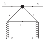
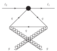
Figure 1: Feynman graphs for the calculation of matching coefficients of gluonic operators. The large dots indicate the effective vertices described by Eq. (1).

By calculating the loop diagrams in Fig. 1, using the standard methods Peskin:1995ev , the coefficients $c_{i}^{\ell_{1}\ell_{2}}$ can be expressed through $C_{i}^{q\ell_{1}\ell_{2}}$ in Eq. (1) as

$$c_{1}^{\ell_{1}\ell_{2}} = -\frac{2}{9}\sum_{q=c,b,t}\frac{I_{1}(m_{q})}{m_{q}}(C_{1}^{q\ell_{1}\ell_{2}}+C_{2}^{q\ell_{1}\ell_{2}}),$$ (9)

$$c_{2}^{\ell_{1}\ell_{2}} = \frac{2\text{i}}{9}\sum_{q=c,b,t}\frac{I_{2}(m_{q})}{m_{q}}(C_{1}^{q\ell_{1}\ell_{2}}-C_{2}^{q\ell_{1}\ell_{2}}),$$ (10)

$$c_{3}^{\ell_{1}\ell_{2}} = -\frac{2}{9}\sum_{q=c,b,t}\frac{I_{1}(m_{q})}{m_{q}}(C_{3}^{q\ell_{1}\ell_{2}}+C_{4}^{q\ell_{1}\ell_{2}}),$$ (11)

$$c_{4}^{\ell_{1}\ell_{2}} = \frac{2\text{i}}{9}\sum_{q=c,b,t}\frac{I_{2}(m_{q})}{m_{q}}(C_{3}^{q\ell_{1}\ell_{2}}-C_{4}^{q\ell_{1}\ell_{2}}),$$ (12)

where the coefficients (see Ref. Rizzo:1979mf for $I_{1}$ and Appendix A) at the leading order are

$$I_{1}=\frac{1}{3},\quad I_{2}=\frac{1}{2}$$ (13)

Note, as previously discussed, that while the Wilson coefficients in Eq. (9)-(12) explicitly contain factors of $1/m_{q}$, in many models the coefficients $C_{i}^{q\ell_{1}\ell_{2}}$ contain factors of $m_{q}$, which we absorbed as part of their definition. Also, we do not explicitly write out contributions to Wilson coefficients due to possible colored heavy states that are not SM quarks; those contributions would result in additive modifications of Eqs. (9)-(12). Also, in this paper, we ignored running of $c_{i}$ in between different scales.

Integrating out heavy particles could also result in higher dimensional gluonic operators, as would happen for vector-like dimension-6 operators. For instance, a set of operators of dimension 8 can be written as

$$O_{1}^{(8)} = \epsilon^{\mu\nu\alpha\beta}(\bar{\ell}_{1L}\partial_{\mu}\gamma_{\nu}\ell_{2L})\frac{\beta_{L}}{4\alpha_{s}}G^{a}_{\alpha\rho}G^{a\rho}_{\beta}\,$$

$$O_{2}^{(8)} = \epsilon^{\mu\nu\alpha\beta}(\bar{\ell}_{1L}\partial_{\mu}\gamma^{\rho}\ell_{2L})\frac{\beta_{L}}{4\alpha_{s}}G^{a}_{\rho\nu}G^{a}_{\alpha\beta}\,$$ (14)

$$O_{3}^{(8)} = \qquad~{}(\bar{\ell}_{1L}\partial_{\mu}\gamma^{\rho}\ell_{2L})\frac{\beta_{L}}{4\alpha_{s}}G_{\rho\alpha}\widetilde{G}^{a\mu\alpha}\,$$

Another three operators, $O_{4}^{(8)}-O_{6}^{(8)}$ could be obtained by substituting left-handed lepton fields with the right-handed ones. Here we shall concentrate on the operators of dimension 7, leaving analysis of higher-dimensional operator for future work.

This paper is organized as follows. In section II we reexamine constraints on the Wilson coefficients of operators $O_{1}^{e\mu}$ and $O_{3}^{e\mu}$ from $\mu$-$e$ conversion data. We consider constraints on Wilson coefficients of operators $O_{1}^{\ell\tau}-O_{4}^{\ell\tau}$ from tau decays in section III. As an example, in section IV we consider how our constraints translate into constraints on couplings of LFV lepton currents with heavy quarks in leptoquark models. We conclude in section V .

II Constraints from $\mu$-$e$ conversion

Muon conversion on a nucleus Marciano:1977cj ; Shanker:1979ap ; Vergados:1985pq ; Bernabeu:1993ta ; Kosmas:1993ch ; Barbieri:1994pv ; Barbieri:1995tw offers a sensitive probe of new physics and a nice possibility to study it experimentally providing an interesting interplay of particle and nuclear physics effects. The number of relevant operators in Eqs. (1) and (5) is reduced if one only considers coherent $\mu+N\to e+N$ transitions Cirigliano:2009bz .

The initial state in the $\mu$-$e$ conversion process

$$\mu^{-}+(A,Z)\to e^{-}+(A,Z)^{\prime}$$ (15)

is the $1s$ state of the muonic atom with the binding energy $E_{b}$, and the final electron state is the eigenstate with the energy $m_{\mu}-E_{b}$ (neglecting the atomic recoil energy of a muonic atom, see Bertl:2006up ). Following Ref. Kitano:2002mt the $\mu$-$e$ conversion amplitude can be written as

$$M_{NN^{\prime}}^{\mu e} = \frac{1}{\Lambda^{2}}\int d^{3}x\left[\left(c_{1}\bar{\psi}_{\kappa,W}^{\mu(e)}P_{L}\psi_{1s}^{(\mu)}\right.\right.$$ (16)

$$+ \left.c_{3}\bar{\psi}_{\kappa,W}^{\mu(e)}P_{R}\psi_{1s}^{(\mu)}\right)\langle N^{\prime}|\frac{\beta_{L}}{4\alpha_{s}}G_{\mu\nu}^{a}G^{a\mu\nu}|N\rangle$$

$$+ \left(c_{2}\bar{\psi}_{\kappa,W}^{\mu(e)}P_{L}\psi_{1s}^{(\mu)}+c_{4}\bar{\psi}_{\kappa,W}^{\mu(e)}P_{R}\psi_{1s}^{(\mu)}\right)$$

$$\times \left.\langle N^{\prime}|\frac{\beta_{L}}{4\alpha_{s}}G_{\mu\nu}^{a}\widetilde{G}^{a\mu\nu}|N\rangle\right],$$

where $\langle N^{\prime}|$ and $|N\rangle$ are the final and initial states of the nucleus, respectively; the $1s$ initial muon wave function

$$\psi_{1s}^{(\mu)}=\left(\begin{array}[]{c}g_{\mu}^{-}\chi_{-1}^{\pm 1/2}\\ \text{i}f_{\mu}^{-}\chi_{1}^{\pm 1/2}\\ \end{array}\right)$$ (19)

is normalized to 1 and corresponds to the quantum numbers $\kappa=-1$ and $\mu=\pm 1/2$ of the operators

$$K=\left(\begin{array}[]{cc}{\boldsymbol{\sigma}}\cdot{\boldsymbol{\it l}}+1&0\\ 0&-({\boldsymbol{\sigma}}\cdot{\boldsymbol{\it l}}+1)\\ \end{array}\right)$$ (22)

and $j_{z}$, respectively, where ${\boldsymbol{\it l}}$ is the orbital angular momentum; and $\kappa=\pm 1$ final electron wave functions

$$\psi_{-1,W}^{\pm 1/2(e)}=\left(\begin{array}[]{c}g_{e}^{-}\chi_{-1}^{\pm 1/2}\\ \text{i}f_{e}^{-}\chi_{1}^{\pm 1/2}\\ \end{array}\right)$$ (25)

and

$$\psi_{1,W}^{\pm 1/2(e)}=\left(\begin{array}[]{c}g_{e}^{+}\chi_{1}^{\pm 1/2}\\ \text{i}f_{e}^{+}\chi_{-1}^{\pm 1/2}\\ \end{array}\right)$$ (28)

are normalized as

$$\int d^{3}x\ \psi_{\kappa,W}^{\mu(e)*}({\bf x})\psi_{\kappa^{\prime},W^{\prime}}^{\mu^{\prime}(e)}({\bf x})=2\pi\delta_{\mu\mu^{\prime}}\delta_{\kappa\kappa^{\prime}}\delta(W-W^{\prime}),$$ (29)

where $W$ is the energy. The electron mass was neglected in Eqs. (25) and (28) so that $g_{e}^{+}=\text{i}f_{e}^{-}$ and $\text{i}f_{e}^{+}=g_{e}^{-}$. Using the normalization

$$\int_{-1}^{1}d\cos\theta\int_{0}^{2\pi}d\phi\chi_{\kappa}^{\mu*}\chi_{\kappa^{\prime}}^{\mu^{\prime}}=\delta_{\mu\mu^{\prime}}\delta_{\kappa\kappa^{\prime}}$$ (30)

of the eigenfunctions $\chi_{\kappa}^{\mu}$ of $({\boldsymbol{\sigma}}\cdot{\boldsymbol{\it l}}+1)$ and $j_{z}$, we have

$$\bar{\psi}_{-1,W}^{(e)}P_{\alpha}\psi_{1s}^{(\mu)} = \frac{1}{2}\left(g_{e}^{-}g_{\mu}^{-}-f_{e}^{-}f_{\mu}^{-}\right)$$ (31)

$$= \bar{\psi}_{1,W}^{(e)}P_{R}\psi_{1s}^{(\mu)},$$

$$\bar{\psi}_{1,W}^{(e)}P_{L}\psi_{1s}^{(\mu)} = -\frac{1}{2}\left(g_{e}^{-}g_{\mu}^{-}-f_{e}^{-}f_{\mu}^{-}\right)$$ (32)

with $\alpha=L,R$.

The pseudoscalar nucleon current couples to the nuclear spin leading to incoherent contribution Kosmas:2001mv . The matrix element in Eq. (16) relevant to the coherent conversion process ($N=N^{\prime}$) can be expressed by the proton $\rho^{(p)}$ and neutron $\rho^{(n)}$ densities in a nucleus as

$$\langle N|\frac{\beta_{L}}{4\alpha_{s}}G_{\mu\nu}^{a}G^{a\mu\nu}|N\rangle$$

$$=-\frac{9}{2}\left[ZG^{(g,p)}\rho^{(p)}+(A-Z)G^{(g,n)}\rho^{(n)}\right],$$ (33)

where $A$ and $Z$ represent mass and atomic number of the nucleus, and the matrix element of gluon operator between the nucleon states is defined as

$$G^{(g,\mathcal{N})}=\langle\mathcal{N}|\frac{\alpha_{s}}{4\pi}G_{\mu\nu}^{a}G^{a\mu\nu}|\mathcal{N}\rangle$$ (34)

with $\mathcal{N}=n,p$. This scalar matrix element can be calculated by using the trace of the energy-momentum tensor $\Theta^{\mu}_{~{}\mu}$ Shifman:1978zn and applying the flavor $SU(3)$ symmetry. Since $\Theta^{\mu}_{~{}\mu}$ is flavor symmetric, the proton and neutron scalar matrix elements are equal. For the strange-quark sigma term $\sigma_{s}\equiv m_{s}\langle p|\bar{s}s|p\rangle=50$ MeV the numerical result is $G^{(g,\mathcal{N})}=-189$ MeV Cheng:2012qr .

The nucleon densities are assumed spherically symmetric and normalized as

$$\int_{0}^{\infty}dr4\pi r^{2}\rho^{(\mathcal{N})}(r)=1.$$ (35)

As usual for spherical nuclei, the two-parameter Fermi (2pF) charge distribution is used

$$\rho(r)=\frac{\rho_{0}}{1+\exp[(r-c)/z]},$$ (36)

where $c$ is the half-density radius.

The formula for the coherent conversion rate can be written as

$$\Gamma_{\text{conv}}(\mu N\to eN)=\frac{4}{\Lambda^{4}}\left(|c_{1}|^{2}+|c_{3}|^{2}\right)a_{N}^{2},$$ (37)

where

$$a_{N}=G^{(g,p)}S^{(p)}+G^{(g,n)}S^{(n)}.$$ (38)

The overlap integrals are defined as Kitano:2002mt

$$S^{(p)}=\frac{1}{2\sqrt{2}}\int_{0}^{\infty}drr^{2}Z\rho^{(p)}(g_{e}^{-}g_{\mu}^{-}-f_{e}^{-}f_{\mu}^{-}),$$ (39)

$$S^{(n)}=\frac{1}{2\sqrt{2}}\int_{0}^{\infty}drr^{2}(A-Z)\rho^{(n)}(g_{e}^{-}g_{\mu}^{-}-f_{e}^{-}f_{\mu}^{-}).$$ (40)

The parameters of model 2pF of nucleon densities in Eq. (36) De Jager:1987qc , and the overlap integrals in Eqs. (39) and (40) Kitano:2002mt for the same distributions

$$\rho^{(p)}(r)=\rho^{(n)}(r)\equiv\rho(r)$$ (41)

of neutrons and protons in the nuclei ${}^{48}_{22}$Ti and ${}^{197}_{79}$Au are shown in Table 1.

Table 1: Nucleon densities model parameters, and the overlap integrals in the unit of $m_{\mu}^{5/2}$ for several nuclei

Nucleus	Model	$c$, fm	$z$, fm	$S^{(p)}$	$S^{(n)}$
${}^{48}_{22}$Ti	FB	$-$	$-$	0.0368	0.0435
${}^{197}_{79}$Au	2pF	6.38	0.535	0.0614	0.0918

The parameters of the Fourier-Bessel expansion (FB)

$$\rho(r)=\left\{\begin{array}[]{ccc}\sum\limits_{v}a_{v}\sin(v\pi rR^{-1})/(v\pi rR^{-1})&\text{for}&\ r\leq R\\ 0&\text{for}&\ r>R\\ \end{array}\right.$$ (44)

are given in Ref. De Jager:1987qc ; Fricke:1995zz .

The branching ratio for $\mu$-$e$ conversion on a nucleus $N$ is defined as

$$B_{\mu e}^{N}\equiv\Gamma_{\text{conv}}(\mu^{-}N\to e^{-}N_{\rm g.s.})/\Gamma_{\rm capt}(\mu^{-}{N}),$$ (45)

where g.s. stands for ground state. The SM muon capture rates Suzuki:1987jf ; Kitano:2002mt , the upper bounds on $B_{\mu e}^{N}$, and the binding energies of ${}^{48}_{22}$Ti and ${}^{197}_{79}$Au are given in Table 2 with the respective references.

Table 2: Muon capture rates, bounds on $B_{\mu e}^{N}$, and binding energies for several nuclei $N$

Nucleus	$\Gamma_{\text{capt}}(\mu^{-}N)$, $\text{s}^{-1}$	$B_{\mu e}^{N}$ $(90\%~{}\text{C.L.})$	$E_{b}$, MeV
${}^{48}_{22}$Ti	$2.59\times 10^{6}$	$4.3\times 10^{-12}$ Ref. Dohmen:1993mp	1.25 Ref. Kosmas:1997eca
${}^{197}_{79}$Au	$13.07\times 10^{6}$	$7\times 10^{-13}$ Ref. Bertl:2006up	10.08 Ref. Bertl:2006up

The upper bounds on the parameters of the Lagrangian in Eq. (5) for one nonzero coefficient $c$ at a time are given in Table 3. It shows that the bound on $\mu$-$e$ conversion rate on gold gives the best limit (see also Ref. Harnik:2012pb ).

Table 3: Upper bounds on the parameters of the Lagrangian in Eq. (5) from muon conversion experiments.

Coefficient	Bound on $|c_{i}^{e\mu}|/\Lambda^{2}$, GeV-3
	conversion on ${}^{48}_{22}$Ti	conversion on ${}^{197}_{79}$Au
$c_{1}$	$2.5\times 10^{-11}$	$1.2\times 10^{-11}$
$c_{2}$	$-$	$-$
$c_{3}$	$2.5\times 10^{-11}$	$1.2\times 10^{-11}$
$c_{4}$	$-$	$-$

III Constraints from $\tau$ decays.

The analysis presented above only deals with experimentally-interesting coherent $\mu-e$ conversion. As a result, no parity-violating operator give any contribution to the experimental transition rates. Moreover, we had to resort to models to describe nuclear effects affecting conversion rates. It might be advantageous to use other experimental observables to study LFV new physics couplings to heavy quarks via gluonic operators. LFV tau decays offer such opportunity. Besides, analyses of tau decays have different theoretical uncertainties than muon conversion calculations; in fact, one can use chiral symmetry and low energy theorems to provide model-independent evaluations of operator matrix elements. While the tau decays have been studied in a variety of models Li:2005rr , to the best of our knowledge gluonic operator contribution (and thus constraints on heavy quark couplings from those decays) has not been previously considered. In what follows we shall use tau decays to constrain matrix elements of gluonic operators.

III.1 Parity-conserving gluonic operators

Complimentary to muon conversion experiments considered in section II, parity-conserving operators can also be probed in lepton-flavor-violating tau decays $\tau\to\ell M^{+}M^{-}$, where $\ell=\mu,e$ and $M=\pi,\eta^{(\prime)},K$ Black:2002wh ; Chen:2006hp . In what follows, let us concentrate on the case of three-body decays $\tau\to\mu\pi^{+}\pi^{-}$ and $\tau\to\mu K^{+}K^{-}$, which are the most interesting experimentally since all the final particles are charged. Transitions to other states (like $\tau\to\ell\eta\eta$) can be obtained by employing flavor $SU(3)$ symmetry relations.

In order to constrain the Wilson coefficients of the operators in Eq. (I.1), Eq. (I.1), and Eq. (6) one needs to constrain hadronic matrix elements. For the scalar operators we shall follow Black:2002wh to state

$$\langle\pi^{+}\pi^{-}|\bar{q}q|0\rangle=\langle K^{+}K^{-}|\bar{q}q|0\rangle=\delta^{M}_{q}B_{0},$$ (46)

where for charged final states $\delta^{M}_{q}=1$ if the flavor of the quark field $q$ in the operator matches the flavor content of the meson and zero otherwise. For example, $\langle K^{+}K^{-}|\bar{s}s|0\rangle=\langle K^{+}K^{-}|\bar{u}u|0\rangle=B_{0}$, while $\langle K^{+}K^{-}|\bar{d}d|0\rangle=0$. Matrix elements for other light final states can be related to Eq. (46) via flavor $SU(3)$ relations Black:2002wh , e.g.,

$$3\langle\eta_{8}\eta_{8}|\bar{u}u|0\rangle=\frac{3}{4}\langle\eta_{8}\eta_{8}|\bar{q}q|0\rangle=B_{0}.$$ (47)

Note that $B_{0}=1.96$ GeV can be estimated from the chiral Lagrangian relations, $m_{\pi}^{2}=\left(m_{u}+m_{d}\right)B_{0}$ assuming that $m_{u}=m_{d}=5$ MeV.

For the vector operators Eq. (I.1) one can use the definition of the pion (kaon) form factor and crossing symmetry,

$$\langle M^{+}M^{-}|\bar{q}\gamma_{\mu}q|0\rangle=\delta^{M}_{q}G_{M}^{(q)}(Q^{2})\left(p_{+}-p_{-}\right)_{\mu},$$ (48)

where $Q=p_{\tau}-p_{\ell}$ is the momentum transfer to the hadronic system and $p_{\pm}$ are the 4-momenta of $M^{\pm}$. Note that $G_{M}^{(q)}(0)=1$ Daub:2012mu . Just like before, flavor content of the operators should match that of the final state mesons.

The matrix elements of gluonic operators Eq. (6) are easiest estimated in the chiral limit, where $m_{u}=m_{d}=m_{s}=m_{M}=0$. In that limit, a low-energy theorem states that Voloshin:1985tc

$$\langle M^{+}M^{-}|\frac{\alpha_{s}}{4\pi}G^{a\mu\nu}G_{\mu\nu}^{a}|0\rangle=-\frac{2}{9}q^{2},$$ (49)

We do not expect the results to change much away from the chiral limit, so shall use this estimate in what follows. It is these operators that we are most interested in the paper. Finally, parity invariance of strong interactions implies that

$$\langle M^{+}M^{-}|\bar{q}\gamma_{5}q|0\rangle = \langle M^{+}M^{-}|\frac{\alpha_{s}}{4\pi}G^{a\mu\nu}\widetilde{G}_{\mu\nu}^{a}|0\rangle$$ (50)

$$= \langle M^{+}M^{-}|\bar{q}\gamma_{\mu}\gamma_{5}q|0\rangle=0.$$

With the definitions above one can calculate the differential decay rate for the decay $\tau\to\ell M^{+}M^{-}$. For the scalar and gluonic operators one has

$$\frac{d\Gamma(\tau\to\ell M^{+}M^{-})}{dq^{2}} = \frac{m_{\tau}}{32(2\pi)^{3}\Lambda^{4}}\left[\left|A_{MM}\right|^{2}+\left|B_{MM}\right|^{2}\right]$$ (51)

$$\times \sqrt{1-\frac{4m_{M}^{2}}{q^{2}}}\left(1-\frac{q^{2}}{m_{\tau}^{2}}\right)^{2},$$

where we set $m_{\ell}=0$ and defined

$$A_{MM} = -\frac{2c_{1}^{\ell\tau}}{9}q^{2}+\frac{1}{2}\sum_{q=u,d,s}\left(C_{1}^{q\ell\tau}+C_{2}^{q\ell\tau}\right)\delta^{M}_{q}B_{0},$$

$$B_{MM} = -\frac{2c_{3}^{\ell\tau}}{9}q^{2}+\frac{1}{2}\sum_{q=u,d,s}\left(C_{3}^{q\ell\tau}+C_{4}^{q\ell\tau}\right)\delta^{M}_{q}B_{0}.~{}~{}~{}~{}$$ (52)

Integrating Eq. (51) we obtain constraints on $c_{1}^{\ell\tau}$ and $c_{3}^{\ell\tau}$ listed in Table 4. Finally, for completion, we present the contribution to the differential decay rate due to vector operators,

$$\frac{d\Gamma_{V}(\tau\to\ell M^{+}M^{-})}{dq^{2}}=\frac{m_{\tau}^{3}}{768\pi^{3}\Lambda^{4}}\left[\left|C_{MM}\right|^{2}+\left|D_{MM}\right|^{2}\right]$$

$$\qquad\times\left(1-\frac{4m_{M}^{2}}{q^{2}}\right)^{3/2}\left(1-\frac{q^{2}}{m_{\tau}^{2}}\right)^{2}\left(1-2\frac{q^{2}}{m_{\tau}^{2}}\right),$$ (53)

where we set $m_{\ell}=0$ and defined

$$C_{MM} = \frac{1}{2}\sum_{q=u,d,s}\left(C_{5}^{q\ell\tau}+C_{6}^{q\ell\tau}\right)\delta^{M}_{q}G_{M}$$

$$D_{MM} = \frac{1}{2}\sum_{q=u,d,s}\left(C_{7}^{q\ell\tau}+C_{8}^{q\ell\tau}\right)\delta^{M}_{q}G_{M}.~{}~{}~{}~{}$$ (54)

This result could be used to constrain Wilson coefficients of vector operators.

Table 4: Upper bounds on the parameters of the Lagrangian in Eq. (5) from tau decay experiments.

	Bound on $|c_{i}^{\ell\tau}|/\Lambda^{2}$, GeV-3
Coef	${\cal B}(\tau\to\mu\ \pi^{+}\pi^{-})$	${\cal B}(\tau\to e\ \pi^{+}\pi^{-})$	${\cal B}(\tau\to\mu K^{+}K^{-})$	${\cal B}(\tau\to eK^{+}K^{-})$	${\cal B}(\tau\to\mu\eta^{\prime})$	${\cal B}(\tau\to e\eta^{\prime})$	${\cal B}(\tau\to\mu\eta)$	${\cal B}(\tau\to e\eta)$
	$<2.1\times 10^{-8}$	$<2.3\times 10^{-8}$	$<4.4\times 10^{-8}$	$<3.3\times 10^{-8}$	$<1.3\times 10^{-7}$	$<1.6\times 10^{-7}$	$<1.3\times 10^{-7}$	$<1.6\times 10^{-7}$
$c_{1}$	$6.8\times 10^{-8}$	$6.5\times 10^{-8}$	$9.4\times 10^{-8}$	$8.2\times 10^{-8}$	$-$	$-$	$-$	$-$
$c_{2}$	$-$	$-$	$-$	$-$	$2.3\times 10^{-7}$	$2.5\times 10^{-7}$	$1.6\times 10^{-7}$	$1.5\times 10^{-7}$
$c_{3}$	$6.8\times 10^{-8}$	$6.5\times 10^{-8}$	$9.4\times 10^{-8}$	$8.2\times 10^{-8}$	$-$	$-$	$-$	$-$
$c_{4}$	$-$	$-$	$-$	$-$	$2.3\times 10^{-7}$	$2.5\times 10^{-7}$	$1.6\times 10^{-7}$	$1.5\times 10^{-7}$

III.2 Parity-violating gluonic operators

Constraints on the parity-violating contributions can be obtained from the lepton-flavor-violating meson and tau decays, $\tau\to\ell M$ and $M\to\mu e$, where $\ell=\mu,e$, and $M=\pi,\eta,\eta^{\prime}$. The analysis of decays involving an $\eta^{\prime}$ is especially interesting, as $\eta^{\prime}$ meson contains considerable amount of “glue”, which makes it possible to constrain gluonic LFV operators resulting from integrating out heavy quarks.

To calculate the decay rates one needs to parameterize the hadronic matrix elements,

$$\langle M(p)|\bar{q}\gamma^{\mu}\gamma_{5}q|0\rangle=-ib_{q}f_{M}^{q}p^{\mu},$$

$$\langle M(p)|\bar{q}\gamma_{5}q|0\rangle=-ib_{q}h_{M}^{q},$$ (55)

$$\langle M(p)|\frac{\alpha_{s}}{4\pi}G^{a\mu\nu}\widetilde{G}^{a}_{\mu\nu}|0\rangle=a_{M},$$

where $q=u,d,s$, and $b_{u,d}=1/\sqrt{2}$, $b_{s}=1$. The form factors defined above in the Feldmann-Kroll-Stech (FKS) mixing scheme Feldmann:1998vh are constrained for $\eta$ and $\eta^{\prime}$ mesons to be Beneke:2002jn

$$a_{\eta} = -\frac{m_{\eta^{\prime}}^{2}-m_{\eta}^{2}}{2}\sin 2\phi\left(-f_{q}b_{q}\sin\phi+f_{s}\cos\phi\right),$$

$$a_{\eta^{\prime}} = -\frac{m_{\eta^{\prime}}^{2}-m_{\eta}^{2}}{2}\sin 2\phi\left(f_{q}b_{q}\sin\phi+f_{s}\cos\phi\right),$$ (56)

where $\phi=39.3^{o}\pm 1.0^{o}$ is a mixing angle of $\eta$ and $\eta^{\prime}$ in the flavor basis Beneke:2002jn . Numerically, anomaly matrix elements are $a_{\eta}=-0.022\pm 0.002$ GeV³, $a_{\eta^{\prime}}=-0.057\pm 0.002$ GeV³. The decays constants in Eq. (III.2) used in numerical work are $f^{q}_{\eta}=108\pm 3$ MeV, $f^{q}_{\eta^{\prime}}=89\pm 3$ MeV, $f^{s}_{\eta}=-111\pm 6$ MeV, and $f^{s}_{\eta^{\prime}}=136\pm 6$ MeV Beneke:2002jn ; Petrov:1997yf .

Neglecting terms of the order ${\cal O}(m_{\ell}/m_{\tau})$, which would change our answer to at most $5\%$ for $\ell=\mu$, we can write for the decay rate,

$$\Gamma\left(\tau\to\mu M\right)=\frac{m_{\tau}}{8\pi\Lambda^{4}}\left[\left|A_{M}\right|^{2}+\left|B_{M}\right|^{2}\right]\left(1-\frac{m_{M}^{2}}{m_{\tau}^{2}}\right)^{2},$$ (57)

where $A_{M}$ and $B_{M}$ are defined as

$$A_{M}=-\frac{2i}{9}c_{2}^{\ell\tau}a_{M} + \sum_{q=u,d,s}\left(C_{2}^{q\ell\tau}-C_{1}^{q\ell\tau}\right)\frac{b_{q}h^{q}_{M}}{4m_{q}}$$

$$+ \frac{1}{2}m_{\mu}\sum_{q=u,d,s}\left(C_{5}^{q\ell\tau}-C_{6}^{q\ell\tau}\right)b_{q}f^{q}_{M}~{}~{}~{}~{}~{}$$

$$- \frac{1}{2}m_{\tau}\sum_{q=u,d,s}\left(C_{7}^{q\ell\tau}-C_{8}^{q\ell\tau}\right)b_{q}f^{q}_{M},$$

$$B_{M}=-\frac{2i}{9}c_{4}^{\ell\tau}a_{M} + \sum_{q=u,d,s}\left(C_{4}^{q\ell\tau}-C_{3}^{q\ell\tau}\right)\frac{b_{q}h^{q}_{M}}{4m_{q}}$$

$$- \frac{1}{2}m_{\tau}\sum_{q=u,d,s}\left(C_{5}^{q\ell\tau}-C_{6}^{q\ell\tau}\right)b_{q}f^{q}_{M}~{}~{}~{}~{}$$

$$+ \frac{1}{2}m_{\mu}\sum_{q=u,d,s}\left(C_{7}^{q\ell\tau}-C_{8}^{q\ell\tau}\right)b_{q}f^{q}_{M}.$$

The current experimental bounds on flavor-violating tau decays allow to put stringent constraints on Wilson coefficients $c_{i}^{\ell\tau}$ Beringer:1900zz . We display them in Table 4. These results, along with the ones displayed in Table 3, can be translated into bounds on flavor-changing interactions of leptons with heavy quarks in particular models. As an example on how this can be done, we consider a generic leptoquark model.

IV Model example: leptoquarks

The Wilson coefficients of effective gluonic operators that were constrained in the previous sections can be used to put bounds on parameters of operators describing lepton interactions with heavy quarks in particular models of NP. Let us provide an example of how this can be done using generic leptoquark model.

The general renormalizable, $B$ and $L$ conserving, and $SU(3)\times SU(2)\times U(1)$ invariant LQ-lepton-quark interactions are given in Refs. Buchmuller:1986zs ; Davidson:1993qk ; Gonderinger:2010yn . The relevant for our considertion scalar LQs ($S$) and vector LQs ($V$) interactions are

$$\mathcal{L}_{S} = \left(\lambda_{LS_{0}}\bar{q}_{L}^{c}\text{i}\tau_{2}\ell_{2L}+\lambda_{RS_{0}}\bar{u}_{R}^{c}\ell_{1R}\right)S_{0}^{\dagger}$$ (60)

$$+ \left(\lambda_{LS_{1/2}}\bar{u}_{R}\ell_{2L}+\lambda_{RS_{1/2}}\bar{q}_{L}\text{i}\tau_{2}\ell_{1R}\right)S_{1/2}^{\dagger}+\text{H.c.},~{}~{}$$

$$\mathcal{L}_{V} = \left(\lambda_{LV_{0}}\bar{q}_{L}\gamma_{\mu}\ell_{2L}+\lambda_{RV_{0}}\bar{d}_{R}\gamma_{\mu}\ell_{1R}\right)V_{0}^{\mu{\dagger}}$$

$$+ \left(\lambda_{LV_{1/2}}\bar{d}_{R}^{c}\gamma_{\mu}\ell_{2L}+\lambda_{RV_{1/2}}\bar{q}_{L}^{c}\gamma_{\mu}\ell_{1R}\right)V_{1/2}^{\mu{\dagger}}+\text{H.c.},$$

where $q$, $u$ and $d$ are doublet, singlet up and singlet down quarks, respectively; we omit flavor indexes, the subindexes 0 and 1/2 indicate $SU(2)$ singlet and doublet LQ, respectively; and couplings $\lambda$ are assumed to be real.

Consider $\mu$-$e$ conversion on ${}^{197}_{79}$Au induced by leptoquark exchange. For the values of the loop integral in Eq. (76) we simply have $I_{1}(m_{t})=I_{1}(m_{b})=I_{1}(m_{c})=0.333$ since the muon mass and the binding energy of the muonic gold are much lower than $c$, $b$ and $t$ quark masses. The expressions for relevant Wilson coefficients in Eq. (1) are given in Table 5, where the quark flavor indexes are $u=u,c,t$ and $d=d,s,b$.

Table 5: The Wilson coefficients for the model with LQs

$C_{i}^{u}/\Lambda^{2}$	Expression	$C_{i}^{d}/\Lambda^{2}$	Expression
$\frac{C_{1}^{u}}{\Lambda^{2}}$	$\frac{\lambda_{RS_{1/2}}^{\ell_{1}u}\lambda_{LS_{1/2}}^{\ell_{2}u}}{2M_{S_{1/2}}^{2}}$	$\frac{C_{1}^{d}}{\Lambda^{2}}$	$\frac{\lambda_{LV_{1/2}}^{\ell_{2}b}\lambda_{RV_{1/2}}^{\ell_{1}b}}{M_{V_{1/2}}^{2}}$
$\frac{C_{2}^{u}}{\Lambda^{2}}$	$\frac{\lambda_{RS_{0}}^{\ell_{1}u}\lambda_{LS_{0}}^{\ell_{2}u}}{2M_{S_{0}}^{2}}$	$\frac{C_{2}^{d}}{\Lambda^{2}}$	$\frac{\lambda_{LV_{0}}^{\ell_{2}b}\lambda_{RV_{0}}^{\ell_{1}b}}{M_{V_{0}}^{2}}$
$\frac{C_{3}^{u}}{\Lambda^{2}}$	$\frac{\lambda_{RS_{0}}^{\ell_{2}u}\lambda_{LS_{0}}^{\ell_{1}u}}{2M_{S_{0}}^{2}}$	$\frac{C_{3}^{d}}{\Lambda^{2}}$	$\frac{\lambda_{LV_{0}}^{\ell_{1}b}\lambda_{RV_{0}}^{\ell_{2}b}}{M_{V_{0}}^{2}}$
$\frac{C_{4}^{u}}{\Lambda^{2}}$	$\frac{\lambda_{RS_{1/2}}^{\ell_{2}u}\lambda_{LS_{1/2}}^{\ell_{1}u}}{2M_{S_{1/2}}^{2}}$	$\frac{C_{4}^{d}}{\Lambda^{2}}$	$\frac{\lambda_{LV_{1/2}}^{\ell_{1}b}\lambda_{RV_{1/2}}^{\ell_{2}b}}{M_{V_{1/2}}^{2}}$

We assume that only the couplings $\lambda$ for a single quark flavor are nonzero at a time. From Eqs. (9) and (11) it follows that the best bounds for the scalar LQs (left half of the Table 5) are relaxed by the factor $2m_{t}/m_{b}\simeq 75$ with respect to the ones for the vector LQs (right half of the Table 5). Using the bound on $|c_{1}|$, we have for $e=\ell_{1}$ and $\mu=\ell_{2}$

$$\frac{|\lambda^{et}_{RS_{0}}\lambda^{\mu t}_{LS_{0}}|}{M_{S_{0}}^{2}}=\frac{|\lambda^{et}_{RS_{1/2}}\lambda^{\mu t}_{LS_{1/2}}|}{M_{S_{1/2}}^{2}}<1.2\times 10^{-8}~{}\text{GeV}^{-2},$$ (62)

$$\frac{|\lambda^{\mu b}_{LV_{0}}\lambda^{eb}_{RV_{0}}|}{M_{V_{0}}^{2}}=\frac{|\lambda^{\mu b}_{LV_{1/2}}\lambda^{eb}_{RV_{1/2}}|}{M_{V_{1/2}}^{2}}<1.6\times 10^{-10}~{}\text{GeV}^{-2},$$ (63)

and, using the bound on $|c_{3}|$, we have

$$\frac{|\lambda^{\mu t}_{RS_{0}}\lambda^{et}_{LS_{0}}|}{M_{S_{0}}^{2}}=\frac{|\lambda^{\mu t}_{RS_{1/2}}\lambda^{et}_{LS_{1/2}}|}{M_{S_{1/2}}^{2}}<1.2\times 10^{-8}~{}\text{GeV}^{-2},$$ (64)

$$\frac{|\lambda^{eb}_{LV_{0}}\lambda^{\mu b}_{RV_{0}}|}{M_{V_{0}}^{2}}=\frac{|\lambda^{eb}_{LV_{1/2}}\lambda^{\mu b}_{RV_{1/2}}|}{M_{V_{1/2}}^{2}}<1.6\times 10^{-10}~{}\text{GeV}^{-2}.$$ (65)

Finally, for the common scales $M_{S}$ and $M_{V}$ of scalar and vector LQ masses, respectively, we get

$$|\lambda^{\alpha t}_{RS_{0}}\lambda^{\beta t}_{LS_{0}}|=|\lambda^{\alpha t}_{RS_{1/2}}\lambda^{\beta t}_{LS_{1/2}}|<1.2\times 10^{-2}~{}\left(\frac{M_{S}}{1~{}\text{TeV}}\right)^{2},$$ (66)

$$|\lambda^{\alpha b}_{LV_{0}}\lambda^{\beta b}_{RV_{0}}|=|\lambda^{\alpha b}_{LV_{1/2}}\lambda^{\beta b}_{RV_{1/2}}|<1.6\times 10^{-4}~{}\left(\frac{M_{V}}{1~{}\text{TeV}}\right)^{2},$$ (67)

where $\alpha\neq\beta=e,\mu$.

In leptoquark models the couplings of heavy quarks can also be constrained from the photon dipole-like operators that also contribute to $\mu\to e\gamma$. Those have been recently constrained in Ref. Gabrielli:2000te . Assuming the dominance of the dipole operator over all other contributions, one obtains comparable bounds on heavy quark couplings to leptoquarks which are of order $10^{-3}(M_{LQ}/1\,{\rm TeV})^{2}$ for the products of couplings with same chiralities $|\lambda_{LQ}^{\mu i}\lambda_{LQ}^{ei}|$. Here we only considered quarks of the last two generations $i=2,3$ (either $c,t$ or $s,b$), $LQ=LS_{0}$, $RS_{0}$, $LS_{1/2}$, $RS_{1/2}$, $LV_{0}$, $RV_{0}$, $LV_{1/2}$ and $RV_{1/2}$, with $M_{LQ}$ being the mass of the correspondent scalar or vector LQ Gabrielli:2000te .

Similar constraints are also available from tau decays. For $\mu=\ell_{1}$ and $\tau=\ell_{2}$

$$\frac{|\lambda^{\mu t}_{RS_{0}}\lambda^{\tau t}_{LS_{0}}|}{M_{S_{0}}^{2}}=\frac{|\lambda^{\mu t}_{RS_{1/2}}\lambda^{\tau t}_{LS_{1/2}}|}{M_{S_{1/2}}^{2}}<2.3\times 10^{-4}~{}\text{GeV}^{-2},$$ (68)

$$\frac{|\lambda^{\tau b}_{LV_{0}}\lambda^{\mu b}_{RV_{0}}|}{M_{V_{0}}^{2}}=\frac{|\lambda^{\tau b}_{LV_{1/2}}\lambda^{\mu b}_{RV_{1/2}}|}{M_{V_{1/2}}^{2}}<4.4\times 10^{-6}~{}\text{GeV}^{-2},$$ (69)

and,

$$\frac{|\lambda^{\tau t}_{RS_{0}}\lambda^{\mu t}_{LS_{0}}|}{M_{S_{0}}^{2}}=\frac{|\lambda^{\tau t}_{RS_{1/2}}\lambda^{\mu t}_{LS_{1/2}}|}{M_{S_{1/2}}^{2}}<2.3\times 10^{-4}~{}\text{GeV}^{-2},$$ (70)

$$\frac{|\lambda^{\mu b}_{LV_{0}}\lambda^{\tau b}_{RV_{0}}|}{M_{V_{0}}^{2}}=\frac{|\lambda^{\mu b}_{LV_{1/2}}\lambda^{\tau b}_{RV_{1/2}}|}{M_{V_{1/2}}^{2}}<4.4\times 10^{-6}~{}\text{GeV}^{-2}.$$ (71)

While for $e=\ell_{1}$ and $\tau=\ell_{2}$,

$$\frac{|\lambda^{et}_{RS_{0}}\lambda^{\tau t}_{LS_{0}}|}{M_{S_{0}}^{2}}=\frac{|\lambda^{et}_{RS_{1/2}}\lambda^{\tau t}_{LS_{1/2}}|}{M_{S_{1/2}}^{2}}<2.2\times 10^{-4}~{}\text{GeV}^{-2},$$ (72)

$$\frac{|\lambda^{\tau b}_{LV_{0}}\lambda^{eb}_{RV_{0}}|}{M_{V_{0}}^{2}}=\frac{|\lambda^{\tau b}_{LV_{1/2}}\lambda^{eb}_{RV_{1/2}}|}{M_{V_{1/2}}^{2}}<4.2\times 10^{-6}~{}\text{GeV}^{-2},$$ (73)

and,

$$\frac{|\lambda^{\tau t}_{RS_{0}}\lambda^{et}_{LS_{0}}|}{M_{S_{0}}^{2}}=\frac{|\lambda^{\tau t}_{RS_{1/2}}\lambda^{et}_{LS_{1/2}}|}{M_{S_{1/2}}^{2}}<2.2\times 10^{-4}~{}\text{GeV}^{-2},$$ (74)

$$\frac{|\lambda^{eb}_{LV_{0}}\lambda^{\tau b}_{RV_{0}}|}{M_{V_{0}}^{2}}=\frac{|\lambda^{eb}_{LV_{1/2}}\lambda^{\tau b}_{RV_{1/2}}|}{M_{V_{1/2}}^{2}}<4.2\times 10^{-6}~{}\text{GeV}^{-2}.$$ (75)

Clearly, constraints on the coefficients of operators containing tau-lepton fields are much weaker than the ones containing muon fields. We expect those constraints to improve with new data coming from Belle II collaboration.

V Conclusions

We considered contributions of heavy quark-induced operators to leptonic FCNC transitions. We constrained Wilson coefficients of effective gluonic operators in $\mu-e$, $\tau-\mu$, and $\tau-e$ transitions. These bounds can be used to study interactions of leptonic FCNCs with heavy quarks that are kinematically inaccessible in the described experiments. We provided an explicit example of constraints on the parameters of a generic leptoquark model.

Appendix A Integrals

In this appendix we present the results of computation of the integrals needed to obtain the matching coefficients of gluonic operators of dimension 7. The matching coefficients can be computed to be

$$I_{1}(m_{q})=\lambda_{q}\int_{0}^{1}dx\int_{0}^{1-x}dy\frac{1-4xy}{\lambda_{q}-xy},$$ (76)

$$I_{2}(m_{q})=\lambda_{q}\int_{0}^{1}dx\int_{0}^{1-x}dy\frac{1}{\lambda_{q}-xy},$$ (77)

where $\lambda_{q}=m_{q}^{2}/E^{2}$ with the process energy scale $E$. For $\lambda_{q}>1/4$ they take the form

$$I_{1} = 2\lambda_{q}-\lambda_{q}(4\lambda_{q}-1)\left[\text{Li}_{2}\left(\frac{1+\text{i}\sqrt{-1+4\lambda_{q}}}{2\lambda_{q}}\right)\right.$$ (78)

$$+ \left.\text{Li}_{2}\left(-\frac{2\text{i}}{\sqrt{-1+4\lambda_{q}}-\text{i}}\right)\right],$$ (79)

$$I_{2} = \lambda_{q}\left[\text{Li}_{2}\left(\frac{1+\text{i}\sqrt{-1+4\lambda_{q}}}{2\lambda_{q}}\right)\right.$$ (80)

$$+ \left.\text{Li}_{2}\left(-\frac{2\text{i}}{\sqrt{-1+4\lambda_{q}}-\text{i}}\right)\right],$$ (81)

for $\lambda_{q}\gg 1$ they are

$$I_{1}=\frac{1}{3}\left[1+\frac{7}{120}\lambda_{q}^{-1}+\mathcal{O}(\lambda_{q}^{-2})\right],$$ (82)

$$I_{2}=\frac{1}{2}\left[1+\frac{1}{12}\lambda_{q}^{-1}+\mathcal{O}(\lambda_{q}^{-2})\right].$$ (83)

In this paper we use the leading order result in the $\lambda_{q}$-expansion.

References

• (1) See, e.g., W. J. Marciano and A. I. Sanda, Phys. Lett. B 67, 303 (1977).
• (2) J. D. Vergados, Phys. Rept.  133, 1 (1986).
• (3) V. Cirigliano, R. Kitano, Y. Okada and P. Tuzon, Phys. Rev. D 80, 013002 (2009) [arXiv:0904.0957 [hep-ph]].
• (4) A good example of this approach can be seen in discussion of charm mixing, see, e.g., E. Golowich, J. Hewett, S. Pakvasa and A. A. Petrov, Phys. Rev. D 76, 095009 (2007) [arXiv:0705.3650 [hep-ph]].
• (5) For similar approach to generate lepton flavor-violating transitions with photons in the final state see, e.g. M. Raidal and A. Santamaria, Phys. Lett. B 421, 250 (1998); K. J. Healey, A. A. Petrov and D. Zhuridov, Phys. Rev. D 87, 117301 (2013).
• (6) For example, $Q_{1}$ operator would result from an operator of the form $(\bar{\ell}_{1R}HL_{2L})\ (\bar{q}_{R}HQ_{L})$ (where $L_{2L}$ and $Q_{L}$ are the correspondingly electroweak doublets of leptons and quarks). This is a dimension 8 operator that is suppressed by two powers of the NP scale and two powers of the scale $v$ associated with electroweak symmetry breaking.
• (7) T. P. Cheng and M. Sher, Phys. Rev. D 35, 3484 (1987).
• (8) W. -j. Li, Y. -d. Yang and X. -d. Zhang, Phys. Rev. D 73, 073005 (2006) [hep-ph/0511273].
• (9) For lepton flavor-conserving operators a similar approach is followed in H. Potter and G. Valencia, Phys. Lett. B 713, 95 (2012) [arXiv:1202.1780 [hep-ph]]. In that paper the scale $\Lambda$ denotes a combination of a new physics scale, electroweak scale, and scales associates with heavy quark masses.
• (10) M. E. Peskin and D. V. Schroeder, “An Introduction to quantum field theory,” Reading, USA: Addison-Wesley (1995) 842 p.; R. N. Cahn, “A Higgs primer,” LBL-29789.
• (11) T. G. Rizzo, Phys. Rev. D 22, 178 (1980) [Addendum-ibid. D 22, 1824 (1980)].
• (12) W. J. Marciano and A. I. Sanda, Phys. Rev. Lett.  38, 1512 (1977).
• (13) O. U. Shanker, Phys. Rev. D 20, 1608 (1979).
• (14) J. Bernabeu, E. Nardi and D. Tommasini, Nucl. Phys. B 409, 69 (1993) [hep-ph/9306251].
• (15) T. S. Kosmas, G. K. Leontaris and J. D. Vergados, Prog. Part. Nucl. Phys.  33, 397 (1994) [hep-ph/9312217].
• (16) R. Barbieri and L. J. Hall, Phys. Lett. B 338, 212 (1994) [hep-ph/9408406].
• (17) R. Barbieri, L. J. Hall and A. Strumia, Nucl. Phys. B 445, 219 (1995) [hep-ph/9501334].
• (18) For a recent review see, for example, A. Czarnecki, W. J. Marciano and K. Melnikov, AIP Conf. Proc.  435, 409 (1998) [hep-ph/9801218].
• (19) W. H. Bertl et al. [SINDRUM II Collaboration], Eur. Phys. J. C 47, 337 (2006).
• (20) R. Kitano, M. Koike and Y. Okada, Phys. Rev. D 66, 096002 (2002) [Erratum-ibid. D 76, 059902 (2007)] [hep-ph/0203110].
• (21) T. S. Kosmas, S. Kovalenko and I. Schmidt, Phys. Lett. B 511, 203 (2001) [hep-ph/0102101].
• (22) M. A. Shifman, A. I. Vainshtein and V. I. Zakharov, Phys. Lett. B 78, 443 (1978).
• (23) H.-Y. Cheng and C.-W. Chiang, JHEP 1207, 009 (2012) [arXiv:1202.1292 [hep-ph]].
• (24) H. De Vries, C. W. De Jager and C. De Vries, Atom. Data Nucl. Data Tabl.  36, 495 (1987).
• (25) G. Fricke et al., Atom. Data Nucl. Data Tabl.  60, 177 (1995).
• (26) T. Suzuki, D. F. Measday and J. P. Roalsvig, Phys. Rev. C 35, 2212 (1987).
• (27) R. Harnik, J. Kopp and J. Zupan, JHEP 1303, 026 (2013) [arXiv:1209.1397 [hep-ph]].
• (28) C. Dohmen et al. [SINDRUM II. Collaboration], Phys. Lett. B 317, 631 (1993).
• (29) T. S. Kosmas, A. Faessler, F. Simkovic and J. D. Vergados, Phys. Rev. C 56, 526 (1997) [nucl-th/9704021].
• (30) D. Black, T. Han, H. -J. He and M. Sher, Phys. Rev. D 66, 053002 (2002).
• (31) C. -H. Chen and C. -Q. Geng, Phys. Rev. D 74, 035010 (2006).
• (32) For more elaborate studies of hadronic effects, see J. T. Daub, H. K. Dreiner, C. Hanhart, B. Kubis and U. G. Meissner, JHEP 1301, 179 (2013).
• (33) M. B. Voloshin, Sov. J. Nucl. Phys.  44, 478 (1986) [Yad. Fiz.  44, 738 (1986)].
• (34) T. Feldmann, P. Kroll and B. Stech, Phys. Rev. D 58, 114006 (1998).
• (35) M. Beneke and M. Neubert, Nucl. Phys. B 651, 225 (2003) [hep-ph/0210085].
• (36) A. A. Petrov, Phys. Rev. D 58, 054004 (1998)
• (37) J. Beringer et al. [Particle Data Group Collaboration], Phys. Rev. D 86, 010001 (2012), see also Y. Amhis et al. [Heavy Flavor Averaging Group Collaboration], arXiv:1207.1158 [hep-ex]; Y. Miyazaki et al. [Belle Collaboration], Phys. Lett. B 719, 346 (2013).
• (38) W. Buchmuller, R. Ruckl and D. Wyler, Phys. Lett. B 191, 442 (1987) [Erratum-ibid. B 448, 320 (1999)].
• (39) S. Davidson, D. C. Bailey and B. A. Campbell, Z. Phys. C 61, 613 (1994) [hep-ph/9309310].
• (40) M. Gonderinger and M. J. Ramsey-Musolf, JHEP 1011, 045 (2010) [Erratum-ibid.  1205, 047 (2012)] [arXiv:1006.5063 [hep-ph]].
• (41) E. Gabrielli, Phys. Rev. D 62, 055009 (2000) [hep-ph/9911539].