Improved mass measurement using the boundary of many-body phase space

Abstract

We show that mass measurements for new particles appearing in decay chains can be improved by determining the boundary of the available phase space in its full dimensionality rather than by using one-dimensional kinematic features for each stage of the cascade decay. This is demonstrated for the case of one particle decaying to three visible and one invisible particles in a two-stage cascade, but our methods also apply to a more general set of decay topologies. We show that not only mass differences, but also the overall scale of masses can be determined with high precision without having to rely on cross section information. The improvement arises from the properties of the higher dimensional phase space itself, independent of the matrix element for the decay, and it is not weakened by the presence of intermediate on-shell particles in the cascade. Our results are particularly significant for the case of low signal statistics, a distinct possibility for new physics searches in the near future.

I Introduction

The LHC experiments have collected and analyzed roughly 5 fb^-1 of data for 7 TeV collisions and 20 fb^-1 of data for 8 TeV collisions, with no obvious evidence of physics beyond the Standard Model (SM). In many cases, limits on new colored states reach beyond a TeV. It is then important to consider the possibility that colored new states appear at higher energies than expectations based on minimal tuning would imply. Mass limits on color-neutral final states are weaker, but these are also produced with a lower cross section. Therefore, even with the high energy run of the LHC it is quite possible that if we encounter physics beyond the SM, we will only have a limited number of signal events to study it. More quantitatively, with 100 fb^-1 of integrated luminosity at the LHC with 14 TeV collisions, one would produce only $\mathcal{O}(10^{3})$ events with pairs of 1 TeV stops Beenakker et al. (1998), or $\mathcal{O}(10^{4})$ events from electroweak pair production of 300 GeV charginos/neutralinos Beenakker et al. (1999). Moreover, the number of events will decrease further due to selection cuts and branching fractions. Therefore, optimizing measurements such as mass determination for low statistics scenarios becomes crucial. The goal of this paper is to demonstrate that in cascade decays this can be achieved by determining the boundary of the kinematically accessible phase space in its full dimensionality.

The collider phenomenology of most extensions of the SM is dominated by a ${\mathbb{Z}}_{2}$ symmetry. Once ${\mathbb{Z}}_{2}$-odd particles are produced in pairs, they will decay through a sequence of two and three-body decays until the lightest ${\mathbb{Z}}_{2}$-odd particle is reached, which is stable and escapes detection. Resonances are not directly observable in such decay chains, so for the determination of the masses in the decay chain one has to rely on kinematic edges and endpoints, maximal values in the distribution of $(p_{i}+p_{j})^{2}$, where $p_{i}^{\mu}$ and $p_{j}^{\mu}$ are the four-momenta of visible particles emitted in subsequent stages of the decay. The position of each such kinematic feature potentially offers a nontrivial relation between the masses of the intermediate particles in the relevant stage of the decay chain. Aside from matrix-element effects such as spin correlations, the stages of the decay occur independently, and therefore these kinematic features are studied independently for each stage in the cascade decay.

An important weakness of kinematic edges and endpoints, the simplest one-dimensional kinematic observables, is that while they are sensitive to the differences between the unknown masses in the spectrum, they have a “flat direction” along the overall scale of masses. In other words, as all masses in the spectrum are raised and lowered together, edges and endpoints have reduced sensitivity. While using the cross section information may be used to gain additional sensitivity to the overall mass scale, this approach is often unreliable due to unknown theory parameters, especially when the underlying model for the new physics is not known in full detail. In this paper we will show that the method of using the full phase space density can yield a more precise determination of the overall scale of masses compared to kinematic edges and endpoints.

Many methods have been developed over the years for the determination of masses of unknown particles in cascade decays. Beyond the simplest edge/endpoint methods Hinchliffe et al. (1997); Bachacou et al. (2000); Allanach et al. (2000); Lester (2001); Gjelsten et al. (2004, 2005); Lester et al. (2006); Miller et al. (2006); Lester (2007); Ross and Serna (2008); Tovey (2008); Barr et al. (2008a, 2009a); Webber (2009) these include polynomial methods Hinchliffe and Paige (1999); Nojiri et al. (2003); Kawagoe et al. (2005); Gjelsten et al. (2006); Cheng et al. (2007); Nojiri and Takeuchi (2008); Cheng et al. (2008, 2009); Matchev et al. (2009); Autermann et al. (2009); Kim (2010); Han et al. (2010); Kang et al. (2010a); Webber (2009); Nojiri et al. (2010); Kang et al. (2010b); Hubisz and Shao (2011); Cheng et al. (2010); Gripaios et al. (2011); Han et al. (2013a, b), and the use of observables that are not fully Lorentz-invariant but are nevertheless invariant under boosts along the beam direction Lester and Summers (1999); Barr et al. (2003); Meade and Reece (2006); Baumgart et al. (2007); Matsumoto et al. (2007); Lester and Barr (2007); Cho et al. (2008a); Gripaios (2008); Nojiri et al. (2008a); Tovey (2008); Cho et al. (2008b); Serna (2008); Barr et al. (2008a); Nojiri et al. (2008b); Cho et al. (2009a); Cheng and Han (2008); Choi et al. (2009); Matchev and Park (2011); Cohen et al. (2010); Polesello and Tovey (2010); Konar et al. (2010a, b); Curtin (2012); Nojiri and Sakurai (2010); Lester (2011); Mahbubani et al. (2013), as these are very useful in a hadron collider environment where the longitudinal motion of the center of mass frame cannot be determined (though this may not be essential for mass measurement Agashe et al. (2013a, b)). In mass measurements for known particles such as the top quark, or for specific new physics theories, the matrix element for the decay can yield additional information to increase the precision of the measurement Kondo (1988); Dalitz and Goldstein (1992); Abazov et al. (2004); Artoisenet et al. (2010); Alwall et al. (2011a); Fiedler et al. (2010); Gainer et al. (2013); Alwall et al. (2010). However, this is often computationally prohibitive. There are many additional refinements of these ideas, some of which also contain additional information about the overall mass scale in the cascade (for instances in the context of the $M_{T2}$ variable, see Cho et al. (2008c); Barr et al. (2008b, 2009b); Cho et al. (2008a); Barr et al. (2008b); Burns et al. (2009a, b); Cho et al. (2009b) and references therein).

The reader will note that some of the references cited above do indeed have sensitivity to the overall mass scale. It is certainly possible to design one-dimensional observables that are optimized for measuring the overall mass scale. Often, this utilizes the same type of correlations in the full phase space distribution as the multi-dimensional analysis we propose. In this paper, we will not study any optimized observables but instead we will juxtapose the simplest one-dimensional kinematic observables (kinematic edges and endpoints) with an equivalently simple multidimensional analysis. It will be interesting to compare the full phase space analysis with existing optimized analyses, and to explore the extent to which a multidimensional phase space analysis can be further optimized. We leave this for future work.

The properties of two- and three-body phase space relevant for decays are very well understood and are discussed in textbooks. The Lorentz-invariant two-body phase space is trivial. The three body phase space can be expressed, up to rotational invariance, in terms of two Lorentz invariants, which can be taken to be $m_{12}^{2}$ and $m_{13}^{2}$ where $m_{ij}^{2}=(p_{i}+p_{j})^{2}$. As is well known, this parametrization has the additional useful property that the phase space density is constant,

$$d\Pi_{3}={\rm const.}\times dm^{2}_{12}\ dm^{2}_{13}.$$ (1)

In this paper we will show that when cascade decays are studied stage-by-stage in this fashion, taking advantage of one-dimensional kinematic features at each stage, a certain amount of information is still left unused, namely phase space correlations between different stages in the cascade, which can be used to improve the precision of mass measurements especially at low statistics. We should emphasize here that the correlations in question have to do with the distribution of events in the full-dimensional phase space itself, not with the matrix element of the decay. We will demonstrate further that using the full dimensionality of phase space for mass determination can yield information on the overall scale of masses rather than only the difference of masses in the spectrum, a significant improvement over methods relying on edges and endpoints.

Unlike the three-particle phase space, which has a constant volume element when expressed in terms of the conventional Lorentz-invariant parametrization, the corresponding volume element for $n$-particle phase space will in general be a function of the phase space coordinates. The crucial point that will be made quantitatively in the next section is that when $n=4$, the volume element is actually enhanced near the boundary of the kinematically allowed region. This is ideally suited for a mass measurement, which is mainly an attempt at determining the boundary of kinematically accessible phase space, so a phase space density that is enhanced near the boundary means that a modest number of events can still give a good resolution for the boundary. The enhancement in question is not manifest in the more familiar cartesian parametrization of phase space, namely

$$d\Pi_{n}=\left(\prod_{i}\frac{d^{3}p_{i}}{(2\pi)^{3}2E_{i}}\right)\delta^{4}(p_{0}^{\mu}-\sum_{i}p_{i}^{\mu}).$$ (2)

Furthermore, even when the cascade decay contains intermediate particles that go on-shell, we will show that the enhancement still persists, but only when the full cascade is analyzed at once, thus keeping correlations between different stages of the cascade. Analyzing each stage of the cascade independently by looking for kinematic features in several one-dimensional distributions such as edges and endpoints (henceforth referred to simply as an “endpoint analysis”), does not utilize the full information available in these correlations.

Figure 1: A decay topology where the mother particle $X$ undergoes a two body-decay to the intermediate on-shell particle $Y$, which subsequently decays through an off-shell state to the stable invisible particle $4$. The particles associated with momenta $p_{1,2,3}$ are assumed to be observable SM particles.

Let us demonstrate this point in a specific example, namely the decay topology seen in figure 1. In terms of one-dimensional invariants, one expects an endpoint in $m_{23}$, as well as an edge in $m_{123}$ for each fixed value of $m_{23}$. Now consider the single event depicted in figure 2. The solid curve in this figure indicates the true boundary of the kinematically allowed phase space while the dashed curve indicates the boundary obtained using an incorrect hypothesis for $m_{X}$, $m_{Y}$ and $m_{4}$. Two facts become evident by considering this figure, namely that:

1. The single event by itself is consistent with both mass hypotheses when the $m_{123}^{2}$ and the $m_{23}^{2}$ distributions are considered separately. However, it rules out the incorrect hypothesis when the full dimensionality of the phase space boundary is considered. Thus there is information in the full phase space distribution that is not available to either one of the one-dimensional projections.

2. The event in question does not lie close to the endpoints in the projected distributions onto either the $m_{23}^{2}$ or the $m_{123}^{2}$ directions. Therefore this event will carry little weight in an endpoint analysis. In the case of a modest number of total events, the endpoints of any one-dimensional projection will be poorly populated while the full four-body phase space boundary will be well populated, leading to a more precise mass determination.

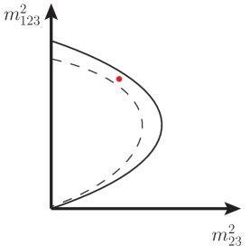
Figure 2: A two-dimensional slice of phase space for the decay topology of figure 1. The solid curve indicates the boundary of the kinematically accessible phase space, and the dashed curve indicates the boundary obtained using an incorrect hypothesis about the unknown masses. The single dot stands for a single decay event.

The rest of this paper will be devoted to quantitatively studying this improvement in the precision of mass measurements at low statistics. We will do this by setting up a comparison between mass measurements for the same underlying physics using multiple endpoint analyses and a single multidimensional analysis (henceforth denoted as “phase space” analysis). In order to focus on the core issue, we will set up this comparison such that many complications that would arise in a realistic study are removed. We will argue below that these simplifying assumptions are not expected to give an advantage to either method of mass measurement and therefore a significant difference in the performance of the methods should persist even as one moves toward a more realistic analysis. The assumptions we make as we set up our analysis are as follows:

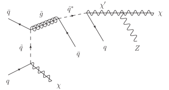
(a)

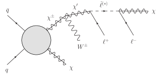
(b)

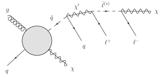
(c)

Figure 3: Production mechanisms in supersymmetric scenarios for which the formalism presented in this paper will be directly applicable.

• For the majority of beyond the SM (BSM) scenarios, the ${\mathbb{Z}}_{2}$ ensures that the particles in the new sector are produced in pairs rather than singly. In order to present as simple an implementation of our methods as possible, we will focus on models where one of the produced particles is the lowest-lying stable particle (LSP) while the other side involves a longer cascade. This choice also reduces the combinatoric background. There are a variety of motivated BSM processes for which such final states are relevant. Here we mention a few examples from supersymmetry:

  1. A spectrum where all scalars super-partners are heavy, and the gluino is light enough to be singly produced in association with the LSP, but too heavy for the pair production to be observable. This is illustrated in figure 3a. Such a spectrum can for instance arise in models of split supersymmetry Arkani-Hamed and Dimopoulos (2005); Giudice and Romanino (2004); Arkani-Hamed et al. (2005, 2012).

  2. A spectrum where all colored states are heavy, but where chargino-neutralino production can allow one to access the electroweak sector. This is illustrated in figure 3b. Here we assume that the chargino is moderately heavy such that the $W$ produced in the cascade is somewhat boosted and can be reconstructed as a single particle. This spectrum can also arise in moderately split models of supersymmetry.

  3. A spectrum where the gluino is very heavy, but squarks are light enough to be produced singly in association with the LSP. If there are further electroweak states between the squark and the LSP, one can easily get longer cascades. This is illustrated in figure 3c.

  In contrast to these asymmetric event topologies, pair production of a heavy particle with long cascade chains on both sides of the event may allow for the events to be fully reconstructed Cheng et al. (2010), or failing that, it is still possible to measure all unknown masses using the methods of ref. Cheng et al. (2007, 2009); Matchev et al. (2009); Autermann et al. (2009); Webber (2009); Nojiri et al. (2010). However, we concentrate on an event topology in this paper that is not easily handled by either one of these methods.

  Finally, there are additional subtleties in the analysis we present when there are cascades on both sides of the event, as additional Lorentz-invariant observables become relevant that are constructed from the momenta coming from opposite sides of the event, thus the phase space distributions of the two mother particles become further correlated with one another. While these subtleties can indeed be addressed within our formalism, this will be left for future work.

• In order to highlight the importance of the phase space density in the mass measurement, we will neglect the effects of spin and assume that all particles in the decay chain decay isotropically. Clearly, this will not be the case for motivated extensions of the SM. We will mention in section V however how spin information could be incorporated for specific models, and may actually be used for the determination of all spins in the cascade, similar to the original Dalitz analysis. In this paper we focus on the determination of the boundary of phase space, while spin determination will deal with the distribution of events throughout phase space, not just the events close to the boundary. The simplifying assumption we make in this paper will allow us to separate these two issues and address the effects of spin in future work.

• We will assume an ideal detector with perfect energy resolution. This is an unrealistic assumption for final state jets, however if the final state particles are leptons or photons, the approximation may be acceptable. In section V we will comment on how the effects of finite energy resolution can be incorporated into the analysis described in section III.

• We will assume that the final state particles are distinguishable. Since we will be dealing with one side of the event only, which contains three visible particles, this assumption is not entirely unrealistic. Nevertheless, we will comment in section V how the analysis may be modified in order to take combinatoric backgrounds into account.

• We will assume that the analysis starts out with the correct hypothesis for the decay topology. This is only a mild assumption, as there are only a few possible topologies in any case. Since our analysis relies on likelihoods, it can in fact be used to compare the quality of fit of alternative hypotheses (see also Bai and Cheng (2011); Birkedal et al. (2005); Costanzo and Tovey (2009); Rajaraman and Yu (2011); Baringer et al. (2011); Choi et al. (2011)). Indeed, multibody phase space correlations are ideal for uncovering the presence of intermediate on-shell particles, since in the narrow-width approximation only certain (hyper)planes of the full phase space will be populated, which can be used to identify the underlying decay topology.

• We will work with a signal-only sample. Clearly, in any realistic analysis, we will need to include SM processes as background that can mimic the relevant final state. Nevertheless, the LHC has already pushed spectra of BSM models to high enough masses that it is plausible to expect that analysis cuts on the transverse momentum of final state particles can yield signal samples with high purity. Furthermore, the likelihood-based analysis we present will not be significantly affected by the presence of such analysis cuts, whereas traditional methods that rely on finding kinematic edges and endpoints may be biased when such cuts are made.

  In any case, it is relatively straightforward to modify our methods to account for the possibility that any given event may have been produced from a background process, and this will be addressed in future work. There is no reason to expect the background to exhibit an enhancement near the boundary of phase space for the signal. Thus the background distribution will be smoothly varying at the boundary of the kinematically allowed phase space, where the signal sample will have an enhancement. This should minimize the impact of background on the applicability of our methods.

We begin by describing in section II the Lorentz-invariant parametrization of phase space for more than three final state particles that is relevant for the rest of our analysis. Then, in section III we describe in detail how we set up the mass measurement, both for the phase space and the endpoint analysis that we use as a reference. We present the results of our analysis for the case of a specific benchmark spectrum in section IV. We conclude in section V, and discuss future directions.

II Description of Four-Particle Phase Space

Our claim that higher precision in mass measurements is possible relies strongly on the fact that the boundary of kinematically accessible phase space is well populated for a single particle decaying to four final states. In order to show that this is indeed the case, this section will be devoted to the description of four-body phase space.

The description of general $n$-particle phase space in terms of Lorentz-invariants was derived in Byers and Yang (1964) and is surprisingly nontrivial. The phase space is described in terms of its boundary and the phase space density. Both of these are written most conveniently by using the following formalism. For final state particles with four momenta $p_{i}^{\mu}$ one begins by introducing the matrix ${\mathcal{Z}}=\{z_{ij}\}$ with $z_{ij}=p_{i}\cdot p_{j}$.

Label by $\Delta_{i}$ the coefficients of the characteristic polynomial of ${\mathcal{Z}}$, namely the equation

$$0 = {\rm Det}\left[\lambda{\rm I}_{n\times n}-{\mathcal{Z}}\right]$$ (3)

$$= \lambda^{n}-\left(\sum_{i=1}^{n}\Delta_{i}\lambda^{n-i}\right).$$

For example, $\Delta_{1}={\rm Tr}[{\mathcal{Z}}]=\sum_{i=1}^{n}m_{i}^{2}$ for any n, and $\Delta_{4}=-{\rm Det}[{\mathcal{Z}}]$ for $n=4$. It is straightforward to show that this definition of $\Delta_{i}$ can also be formulated as

$$\Delta_{l}=(-1)^{l-1}\sum{\rm determinant\ of\ all\ }l\times l{\rm\ diagonal\ minors\ of\ }{\mathcal{Z}}.$$ (4)

The kinematically accessible region for any number $n\geq 4$ particles is then defined by the conditions

$$\begin{array}[]{rl}\Delta_{l}>0&{\rm for\ }l\leq 4\\ \Delta_{l}=0&{\rm for\ }l>4,\end{array}$$ (5)

the boundary of the physical region corresponding to $\Delta_{4}=0$.

The $z_{ij}$ are not all independent variables. For any given set of masses for the initial particle that decays and the final state particles, it is straightforward to count the number of independent phase space coordinates. The energy of each final state particle is fixed by its three-momentum, and there are a total of $3n$ components in the three momenta of the final state particles. The conservation of total energy and momentum for the system allows four of these components to be expressed in terms of the rest, and finally in situations where the decaying particle is a scalar (or its spin states are averaged over), the rotational invariance of the system can be used to eliminate three more degrees of freedom, leaving one with $3n-7$ independent degrees of freedom.

The phase space density is then expressed in terms of the differential volume element $\prod_{i<j}dz_{ij}$, and the reduction to the $3n-7$ independent degrees of freedom proceeds through the inclusion of a number of Dirac-$\delta$ functions. While the form of these $\delta$ functions is rather complicated for arbitrary $n$, it is very simple for $n=4$. For all $n\geq 4$, the volume element includes one $\delta$ function that enforces total energy-momentum conservation in terms of Lorentz-invariant variables. In the case of $n=4$, this is the only $\delta$ function present in the volume element. Indeed, there are 6 $z_{ij}$ with $i<j$, one of which can be eliminated using this $\delta$ function, leaving us with precisely 5 degrees of freedom, the correct number for $3n-7$ when $n=4$.

Before we write down the exact form of the volume element for $n=4$, let us for future convenience switch from the set of variables $z_{ij}$, to $m_{ij}^{2}=(p_{i}+p_{j})^{2}$. Since this is a linear transformation, the functional form of the volume element is unaffected. Without further ado, the volume element of four-body phase space written in terms of Lorentz-invariant observables is

$$d\Pi_{4} =\left(\prod_{i<j}dm_{ij}^{2}\right)\frac{{\rm C}}{M_{X}^{2}\Delta_{4}^{1/2}}\ \delta\left(\sum_{i<j}m_{ij}^{2}-{\rm K}\right),$$ (6)

where $M_{X}$ is the mass of the original particle that decays to the four final states and

$$C=\frac{8}{(4\pi)^{10}}\ ,\qquad K=M_{X}^{2}+2\sum_{i=1}^{4}m_{i}^{2}\ .$$ (7)

As mentioned, this volume element is not flat as in the case of the three-body phase space, but instead depends on the phase space coordinates through the factor of $\Delta_{4}^{-1/2}$ which is a function of the $m_{ij}^{2}$. Since the boundary of the kinematically allowed region is defined by $\Delta_{4}=0$, this means that the phase space density is enhanced near the boundary of the physical region. The apparent singularity is an integrable one, and it is not canceled by the presence of the $\delta$-function enforcing momentum conservation, as its argument is linear in the $m_{ij}^{2}$ and does not lead to any nontrivial Jacobian factors. Of course, in calculating any physical rate, the phase space density is multiplied by the square of the matrix element $|{\mathcal{M}}|^{2}$, and one may worry that on-shell intermediate particles in the cascade, in the narrow width approximation, may manifest themselves as $\delta$-functions in $|{\mathcal{M}}|^{2}$ that may change our conclusions. However, it is easily seen that the momentum going through any on-shell propagator will be a linear combination of the $m_{ij}^{2}$, thus once again these $\delta$ functions will not give rise to any Jacobians that change the functional form of the volume element, and thus cannot modify the enhancement at the boundary of the physical region.

III Analysis Methods

In this section we will outline our analysis strategy and the setup for the comparison with traditional endpoint methods for mass determination. Note that there are only a few possibilities for how a cascade decay to four final state particles may proceed in stages. Denoting the initial particle by $X$, any intermediate resonances by $Y$, $Z$ etc., and the final state particles as 1 through 4, particle 4 always being the invisible one, the possibilities are:

• $X\to 1+Y,\ Y\to 2+Z,\ Z\to 3+4$
  This is a three stage cascade decay, each stage being a two-body decay. We will refer to this possibility as the “2+2+2” topology.

• $X\to 1+Y,\ Y\to 2+3+4$
  This is a two stage cascade decay, with a two-body decay followed by a three-body decay, and is referred to as the “2+3” decay topology.

• $X\to 1+2+Y,\ Y\to 3+4$
  This is a two stage cascade decay, with a three-body decay followed by a two-body decay, and is referred to as the “3+2” decay topology.

• $X\to 1+2+3+4$
  A genuine four-body decay with no intermediate resonances.

The last possibility is essentially never encountered in either the SM or any well-studied BSM scenario, so we will not dwell on it. Furthermore, the third possibility is qualitatively very similar to the second, as we assumed distinguishability of the final state particles. Thus we will not discuss the third possibility separately, and focus our attention on the first two possibilities. These decay topologies are shown in Figure 4. Note that we do not include in our list the “antler” topology, $X\to Y+Z,\ Y\to 1+2,\ Z\to 3+4$. In the literature this topology is only of interest when there are two invisible final state particles, such as particles 2 and 4 for example. Since we are concentrating on the case of a single invisible particle at the end of the cascade, one of the particles $X$ and $Y$ occur as a resonance, and should be considered as a visible final state particle in its own right. Therefore this configuration should strictly speaking be considered a three-body final state rather than a four-body one, and we omit it in our list.

Figure 4: The “2+2+2” and “2+3” decay topologies.

Simply put, in both the phase space and the endpoint analyses, we will study how a set of observed events in the data will favor or disfavor each one of a large number of hypotheses for all unknown masses $\{\tilde{m}_{\sigma}\}\equiv\{\tilde{m}_{X},\tilde{m}_{Y},(\tilde{m}_{Z}),\tilde{m}_{4}\}$. In the case of the phase space analysis, this will be done by using a likelihood, while in the endpoint analysis we will rely on a quality-of fit of the data to any mass hypothesis that is similar to a $\chi^{2}$ variable. We will also study how the performance of the two competing mass determination methods will vary as the number of observed signal events changes, in particular we will be interested in how well the two analyses perform as one moves towards lower statistics.

It should be noted that due to the presence of two on-shell intermediate particles, an event in the 2+2+2 case only has three independent phase space degrees of freedom, and there are three independent observables in the event, namely $m_{12}^{2}$, $m_{13}^{2}$ and $m_{23}^{2}$. Thus for any given mass hypothesis, an event in the 2+2+2 topology can be entirely reconstructed (or it may defy reconstruction, thereby rejecting the mass hypothesis in question). In fact, using information from a small number of events, the unknown masses can be analytically solved for Hinchliffe and Paige (1999); Nojiri et al. (2003); Kawagoe et al. (2005); Gjelsten et al. (2006); Cheng et al. (2007); Nojiri and Takeuchi (2008); Cheng et al. (2008, 2009); Matchev et al. (2009); Autermann et al. (2009); Kim (2010); Han et al. (2010); Kang et al. (2010a); Webber (2009); Nojiri et al. (2010); Kang et al. (2010b); Hubisz and Shao (2011); Cheng et al. (2010); Gripaios et al. (2011); Han et al. (2013a, b). Therefore, for this decay topology our phase space analysis is not particularly useful over the “polynomial method”. However, there is no similar argument for the $2+3$ decay topology, and indeed this is the case which will be our main focus. There is one added subtlety in the 2+3 topology however, which is why we choose to include a discussion of the 2+2+2 topology as a warm-up example to this more interesting case where our methods offer genuine improvement over existing mass determination methods.

In order to estimate the uncertainty in the results of the mass determination procedure, we rely on a large number of pseudoexperiments. Each pseudoexperiment is a data set with a fixed number of events generated with a true mass point $\{M_{\sigma}\}\equiv\{M_{X},M_{Y},(M_{Z}),M_{4}\}$. Based on such a data set, each mass hypothesis (distributed around the true mass point) is assigned a quality-of-fit, which as mentioned is a likelihood in the phase space analysis, and a $\chi^{2}$-like variable in the endpoint analysis. The mass hypothesis with the best quality-of-fit for a given data set is then chosen as the “winner” for that pseudoexperiment. As we repeat this procedure over a large number of pseudoexperiments, a distribution of winning hypotheses emerges. We use the statistical properties of this distribution of winners in order to determine both the central value and the uncertainty of the mass determination procedure.

III.1 Warming Up: The 2+2+2 topology

III.1.1 Analysis using four-body phase space

We set up the likelihood analysis based on the phase space volume element as follows: For an event with kinematic observables $m_{12}^{2},m_{13}^{2}$ and $m_{23}^{2}$ we first use the mass hypothesis $\{\tilde{m}_{\sigma}\}$ and overall energy momentum conservation to solve for $m_{i4}^{2}$. Note that unless the hypothesis used is the true mass point, these will not be the true values of $m_{i4}^{2}$. We then define the likelihood as the normalized probability of obtaining this event given the mass hypothesis $\{\tilde{m}_{\sigma}\}$

$$\mathcal{L}(\tilde{m}_{\sigma},m_{ij}^{2})=\frac{1}{\Gamma_{X}}\frac{1}{2\tilde{m}_{X}}\mu^{2}_{XY1}\mu^{2}_{YZ2}\mu^{2}_{Z34}\frac{\pi}{\tilde{m}_{Y}\Gamma_{Y}}\frac{\pi}{\tilde{m}_{Z}\Gamma_{Z}}\frac{1}{(4\pi)^{6}2\tilde{m}_{X}^{2}}\Theta(\Delta_{4})\frac{1}{\Delta_{4}^{1/2}}.$$ (8)

Several comments are in order. All widths $\Gamma$ as well as $\Delta_{4}$ appearing in this formula are computed with respect to the mass hypothesis $\{\tilde{m}_{\sigma}\}$. The first factor of $\frac{1}{\Gamma_{X}}$ simply ensures that the likelihood is normalized to one for any mass hypothesis

$$\int\mathcal{L}(\tilde{m}_{\sigma},m_{ij}^{2})\ dm_{12}^{2}dm_{13}^{2}dm_{23}^{2}=1.$$ (9)

The factor of $\frac{1}{2\tilde{m}_{X}}$ is simply the prefactor in the definition of a differential width. The trilinear couplings $\mu$ have been labeled in the obvious notation, and have mass dimension one. The factors of $\frac{\pi}{\tilde{m}_{Y}\Gamma_{Y}}$ and $\frac{\pi}{\tilde{m}_{Z}\Gamma_{Z}}$ are simply the remnants of the $Y$ and $Z$ propagators after the narrow width approximation,

$$\frac{1}{|\tilde{m}_{Y}^{2}-(p_{2}+p_{3}+p_{4})^{2}+i\,\tilde{m}_{Y}\Gamma_{Y}|^{2}} \simeq\delta(m_{23}^{2}+m_{24}^{2}+m_{34}^{2}-K_{Y})\frac{\pi}{\tilde{m}_{Y}\Gamma_{Y}},$$

$$\qquad K_{Y}=\tilde{m}_{Y}^{2}+m_{2}^{2}+m_{3}^{2}+m_{4}^{2},$$ (10)

$$\frac{1}{|\tilde{m}_{Z}^{2}-(p_{3}+p_{4})^{2}+i\,\tilde{m}_{Z}\Gamma_{Z}|^{2}} \simeq\delta(m_{34}^{2}-\tilde{m}_{Z}^{2})\frac{\pi}{\tilde{m}_{Z}\Gamma_{Z}}\ .$$ (11)

The factors of $\mu$ and these propagator remnants simply stand for the squared matrix element $|{\mathcal{M}}|^{2}$ when all involved particles are scalars. The remaining factors simply correspond to the phase space volume element given in equation 6. The step function $\Theta(\Delta_{4})$ appears because for an incorrect mass hypothesis, a given event may simply not reconstruct a physical solution, in which case the likelihood evaluates to zero. Note that when finite detector resolution effects are taken into account, the step function needs to be convoluted with the energy resolution of the detector, leading to a smoother turn-off when an event proves difficult to reconstruct. We will come back to this issue in section V.

It is easily seen that there are several cancellations in the likelihood formula between the factors of $\Gamma$ and $\mu^{2}$, leaving only dimensionless functions depending on the masses. In particular, using the respective two-body decay formulae for the widths of $X,Y,Z$, we obtain the final expression for the likelihood

$$\mathcal{L}(\tilde{m}_{\sigma},m_{ij}^{2}) \simeq\frac{1}{4\pi\tilde{m}_{X}^{2}}\left(1-\frac{\tilde{m}_{Y}^{2}}{\tilde{m}_{X}^{2}}\right)^{-1}\left(1-\frac{\tilde{m}_{Z}^{2}}{\tilde{m}_{Y}^{2}}\right)^{-1}\left(1-\frac{\tilde{m}_{4}^{2}}{\tilde{m}_{Z}^{2}}\right)^{-1}\Theta(\Delta_{4})\frac{1}{\Delta_{4}^{1/2}}\,$$ (12)

where we have chosen a simplified form for the dimensionless phase space functions by assuming $m_{1,2,3}\simeq 0$. We use this simpler expression in our analysis, however we do verify numerically that for $m_{1,2,3}\simeq$ few GeV, the difference with the exact result is negligible. The likelihood for the pseudoexperiment is simply the product of likelihoods of each event,

$$\mathcal{L}(\tilde{m}_{\sigma}) =\prod_{events}\mathcal{L}(\tilde{m}_{\sigma},m_{ij}^{2}).$$ (13)

For each pseudoexperiment, the winning mass hypothesis is then chosen as the one that maximizes the above likelihood. In practice we use the log-likeliood and sum over the events in the data sample.

III.1.2 Using edges and endpoints

We want to compare the results of this phase space analysis with those obtained from the endpoint analysis. As noted before, this is not the most optimal analysis for the 2+2+2 topology as the “polynomial method” lets us reconstruct the masses analytically. However, the comparison we set up in this topology will prepare us for the 2+3 topology considered in the next subsection.

The mass determination procedure of the endpoint analysis is based on comparing for each pseudoexperiment the measured position of kinematic features obtained from the data with those that are predicted based on the mass hypothesis being used. In appendix A, we list all the formulae the predicted positions of the kinematic edges and endpoints for this topology using a given mass hypothesis. For the 2+2+2 topology, $Y$ and $Z$ are on-shell, therefore the $m_{12}^{2}$ and $m_{23}^{2}$ distributions have an edge. In contrast, the $m_{13}^{2}$ and $m_{123}^{2}$ distributions have endpoints. The measured positions of the same kinematic edges and endpoints are defined simply as the highest value obtained for the observable in question using all the events in the data set.

We then define the quality-of-fit variable for any mass hypothesis based on a pseudoexperiment as

$$Q =\left(\sum_{i={\rm endpts.}}\left(\frac{\mathcal{O}_{i,predicted}-\mathcal{O}_{i,measured}}{\mathcal{O}_{i,measured}}\right)^{2}\right)\mathcal{F}\,,$$ (14)

where the observables $\mathcal{O}_{i}=\{(m_{123}^{2})_{max},(m_{12}^{2})_{max},(m_{23}^{2})_{max},(m_{13}^{2})_{max}\}$ represent the predicted and measured positions of each edge and endpoint, and the sum is taken over all relevant edges and endpoints. $\mathcal{F}=1$ if all measured endpoints are consistent with the predicted ones, meaning that they occur at smaller (or equal) values of $\mathcal{O}_{i}$. If any one of the measured endpoints exceeds the predicted value, the mass hypothesis is rejected (equivalently, $\mathcal{F}$ is taken to be $\infty$ in that case). As we remarked for the phase space analysis, this sharp step-function behavior will need to be softened once a more realistic model of the detector with finite resolution is used. It should also be remarked here that while it may appear somewhat arbitrary to assign the same weight in $Q$ to the contribution of all edges and endpoints, practically $Q$ is almost always dominated by the position of one of the edges or endpoints, thus the weighting has no significant impact. We dwell on this point in more detail in appendix C.

III.2 Focus Case: The 2+3 topology

We now consider the case where $Y$ has a 3-body decay to $2,3,4$ without an intermediate resonance. The added complication compared to the 2+2+2 topology is that since we have lost the on-shell constraint of $Z$, this event topology is now impossible to reconstruct analytically. In other words, while there are still three observables $m_{ij}^{2}$ as in the 2+2+2 topology, there are now four independent degrees of freedom in the phase space, since only the $Y$ propagator can be used in the narrow width approximation to eliminate one of the phase space integration variables.

III.2.1 Analysis using four-body phase space

One unmeasured phase space variable, which we take to be $m^{2}_{34}$, can no longer be fixed given a mass hypothesis. Hence we integrate over this parameter in the definition of the likelihood. Following the same procedure as earlier, we can use momentum conservation and the on-shell $Y$ propagator to define the likelihood

$$\mathcal{L}(\tilde{m}_{\sigma},m_{ij}^{2})=\frac{1}{\Gamma_{X}}\int dm_{34}^{2}\frac{1}{2\tilde{m}_{X}}\mu^{2}_{XY1}\lambda^{2}_{Y234}\frac{\pi}{\tilde{m}_{Y}\Gamma_{Y}}\frac{1}{(4\pi)^{6}2\tilde{m}_{X}^{2}}\Theta(\Delta_{4})\frac{1}{\Delta_{4}^{1/2}}\ .$$ (15)

Note that $Y$ decays through a quartic scalar coupling which we have labeled as $\lambda$ since it is dimensionless. The factor of $\Theta(\Delta_{4})$ now determines the allowed range of $m_{34}^{2}$ integration, and for an incorrect mass hypothesis it is possible that no value of $m_{34}^{2}$ will lead to a possible reconstruction of the event. As in the 2+2+2 topology, in that case the mass hypothesis may be ruled out with a single event.

The $m_{34}^{2}$ integration can be performed analytically. We present the details of this calculation in appendix B and simply list the result here, which is

$$\mathcal{L}(\tilde{m}_{\sigma},m_{ij}^{2}) =\frac{1}{\Gamma_{X}}\frac{1}{2\tilde{m}_{X}}\mu^{2}_{XY1}\lambda^{2}_{Y234}\frac{\pi}{\tilde{m}_{Y}\Gamma_{Y}}\frac{1}{(4\pi)^{5}2\tilde{m}_{X}^{2}}\frac{1}{\sqrt{\lambda_{0}}}\Theta(-G_{1})\Theta(-G_{2})\,,$$ (16)

where

$$\lambda_{0} =\lambda\left(m_{1}^{2},m_{23}^{2},m_{123}^{2}\right),$$ (17)

$$G_{1} =G\left(m_{12}^{2},m_{23}^{2},m_{123}^{2},m_{2}^{2},m_{1}^{2},m_{3}^{2}\right),$$ (18)

$$G_{2} =G\left(m_{123}^{2},\tilde{m}_{Y}^{2},\tilde{m}_{X}^{2},m_{23}^{2},m_{1}^{2},\tilde{m}_{4}^{2}\right),$$ (19)

and the kinematic functions $\lambda$ and $G$ are defined as Byckling and Kajantie (1973).

$$\lambda(X,Y,Z) =X^{2}+Y^{2}+Z^{2}-2XY-2YZ-2ZX,$$

$$G(X,Y,Z,U,V,W) =XY(X+Y-Z-U-V-W)+ZU(Z+U-X-Y-V-W)$$

$$+VW(V+W-X-Y-Z-U)+XZW+XUV+YZV+YUW.$$ (20)

The likelihood is normalized to 1 as in the 2+2+2 case.

Again using a somewhat more simplified expression assuming $m_{1,2,3}\simeq 0$, and canceling factors of $\Gamma$ against $\mu^{2}$ and $\lambda^{2}$, we can rewrite this as

$$\mathcal{L}(\tilde{m}_{\sigma},m_{ij}^{2}) \simeq\frac{1}{2\tilde{m}_{X}^{2}}\left(1-\frac{\tilde{m}_{Y}^{2}}{\tilde{m}_{X}^{2}}\right)^{-1}\frac{1}{\tilde{m}_{Y}^{2}}\left(1-\frac{\tilde{m}_{4}^{4}}{\tilde{m}_{Y}^{4}}-2\frac{\tilde{m}_{4}^{2}}{\tilde{m}_{Y}^{2}}\log\left(\frac{\tilde{m}_{Y}^{2}}{\tilde{m}_{4}^{2}}\right)\right)^{-1}\times$$

$$\qquad\qquad\qquad\qquad\qquad\qquad\qquad\qquad\qquad\Theta(-G1)\Theta(-G2)\frac{1}{\sqrt{\lambda_{0}}}.$$ (21)

As before, the likelihood for the pseudoexperiment is simply the product of the likelihoods for each event,

$$\mathcal{L}(\tilde{m}_{\sigma}) =\prod_{events}\mathcal{L}(\tilde{m}_{\sigma},m_{ij}^{2}).$$ (22)

III.2.2 Using edges and endpoints

Unlike the case of the phase space analysis, the endpoint analysis for the 2+3 topology is not significantly different than in the 2+2+2 topology. The absence of $Z$ as an on-shell state demotes the edges in the $m_{12}^{2}$ and $m_{23}^{2}$ distributions to endpoints, but the quality-of-fit variable $Q$ is defined in the same way as in equation 14. Since our focus is on situations with low statistics, this often means that the endpoint is not well populated, leading to a large underestimation of the measured endpoint position. Therefore, we expect the results in this case to be less accurate than those for the 2+2+2 topology.

We discuss the results for all analyses described above in detail in the next section using a specific choice of true mass point $\{M_{\sigma}\}$.

IV Results

After having outlined the theoretical details of the analysis we wish to set up, we now turn to the practical implementation and report our results in this section.

The data samples on which we run both the endpoint and the phase space analyses are generated at the parton level using MadGraph 5 Alwall et al. (2011b). As mentioned in the introduction, in order to separate the effects of spin-correlations from the effects of the phase space density, we choose all particles as scalars in the MadGraph model, and we choose one specific mass spectra to use as benchmarks in the analysis of each one of the two decay topologies. All analyses rely on parton-level events as we have chosen to work with a detector with perfect resolution.

IV.1 The 2+2+2 Topology

We work with the benchmark spectrum

$$M_{X} =500\textrm{ GeV}\,,\qquad M_{Y}=350\textrm{ GeV}\,,$$

$$M_{Z} =200\textrm{ GeV}\,,\qquad M_{4}=100\textrm{ GeV}\,,$$

$$m_{1}=m_{2}=m_{3}=5\textrm{ GeV}\,,$$ (23)

and for each pseudoexperiment we use data samples with $N_{events}=100$.

In both the phase space and the endpoint analyses, we also need a set of mass hypotheses $\{\tilde{m}_{\sigma}\}$ from which one is chosen as the winner of each pseudoexperiment. In order to get an accurate picture of the uncertainty in the mass measurement, we check that the range of the set of mass hypotheses is large enough such that a further enlargement would have no effect. In particular, we verify that the flat direction does not extend past the boundaries of the chosen set of mass hypotheses. Below we list how we choose the set of mass hypotheses for both analysis methods, and we later confirm as we list the results of our analysis that the chosen sets indeed satisfy this criterion.

We choose a set of mass hypotheses for the analysis such that the expected flat direction, where all hypothesis masses are raised or lowered together, is well populated and finely scanned. Thus, instead of generating a set of mass hypotheses that lie on a (hyper)cubic lattice in the $\{\tilde{m}_{X},\tilde{m}_{Y},\tilde{m}_{Z},\tilde{m}_{4}\}$ basis, we generate a lattice along a different set of axes, namely:

$$\tilde{m}_{\sigma}=M_{\sigma}+(100~{}{\rm GeV})\left(\alpha V_{\sigma}^{(1)}+\beta V_{\sigma}^{(2)}+\gamma V_{\sigma}^{(3)}+\delta V_{\sigma}^{(4)}\right)\qquad\sigma=\{X,Y,Z,4\}\,,$$ (24)

where

$$V_{\sigma}^{(1)} = \{1,1,1,1\},$$

$$V_{\sigma}^{(2)} = \{1,-1,0,0\},$$

$$V_{\sigma}^{(3)} = \{1,1,-1,-1\},$$

$$V_{\sigma}^{(4)} = \{0,0,1,-1\}\,.$$ (25)

Note that these vectors are chosen to give an orthogonal basis. $V_{\sigma}^{(1)}$ is the vector that corresponds to the flat direction. For the endpoint analysis, we use the following scan for $\alpha,\beta,\gamma,\delta$,

$$\alpha \in[-1,7],$$

$$\beta,\gamma,\delta \in[-0.3,0.3],$$

$$\Delta\alpha =\Delta\beta=\Delta\gamma=\Delta\delta=0.02\,.$$ (26)

Any choice of $(\alpha,\beta,\gamma,\delta)$ is discarded for which the inequality $\tilde{m}_{X}>\tilde{m}_{Y}>\tilde{m}_{Z}>\tilde{m}_{4}>0$ is violated. We have chosen to scan a much wider interval for $\alpha$ in order to accurately sample the flat direction.

For the phase space analysis, we provide results from a much finer scan in a narrow range (after verifying that all winning hypotheses indeed lie in this narrow range). For this case we choose

$$\alpha \in[-1.5\times 10^{-2},1.5\times 10^{-2}] \Delta\alpha =10^{-3},$$

$$\beta,\gamma,\delta \in[-1.5\times 10^{-3},1.5\times 10^{-3}] \Delta\beta =\Delta\gamma=\Delta\delta=10^{-4}.$$ (27)

Mass (GeV)	Phase space	End-points
$m_{X}$	$499.89\pm 0.60$	$677.41\pm 157.47$
$m_{Y}$	$349.90\pm 0.59$	$527.19\pm 155.96$
$m_{Z}$	$199.92\pm 0.59$	$380.11\pm 160.57$
$m_{4}$	$99.93\pm 0.65$	$277.87\pm 156.42$
$\alpha$	$(-0.87\pm 6.03)\times 10^{-3}$	$1.78\pm 1.58$
$\beta$	$(-0.07\pm 0.38)\times 10^{-3}$	$(0.11\pm 1.54)\times 10^{-2}$
$\gamma$	$(-0.17\pm 0.44)\times 10^{-3}$	$(-0.84\pm 1.44)\times 10^{-2}$
$\delta$	$(-0.09\pm 0.66)\times 10^{-3}$	$(1.12\pm 3.08)\times 10^{-2}$

Table 1: Mean and standard deviation of the distribution of winning mass hypotheses across pseudoexperiments using the phase space and endpoint analyses for the 2+2+2 topology. The number of events in each pseudoexperiment was chosen to be $N_{events}=100$.

Having chosen a benchmark spectrum and a set of mass hypotheses, we proceed to run both the phase space and endpoint analyses on ${\mathcal{O}}(10^{3})$ pseudoexperiments. The winner of each pseudoexperiment is chosen in the two analyses as explained in detail in the previous section. In figure 5 and 6 we plot the distribution of winning mass hypotheses in the two analyses. We also list the mean and standard deviation in the distribution of these quantities in table 1. The difference in sensitivity between the two analysis methods is dramatic. Perhaps most importantly, one can observe that the phase space analysis based on the four-body phase space has much better resolution along the flat direction that causes the endpoint analysis results to acquire an enormous spread and bias.

We should note that the standard deviations of the distribution of winners in the $(\alpha,\beta,\gamma,\delta)$ parametrization give a clearer indication of the inherent uncertainty in the mass determination between these two methods. The standard deviations in the distribution of winners in the $\{\tilde{m}_{X},\tilde{m}_{Y},\tilde{m}_{Z},\tilde{m}_{4}\}$ parametrization on the other hand should not be regarded as independent measurement uncertainties since they are all dominated by the spread along the flat direction scanned by $\alpha$.

In appendix C we investigate the endpoint analysis along the flat direction in further detail, and show why it produces a poor result at low statistics, and furthermore exhibits a bias towards higher mass values.

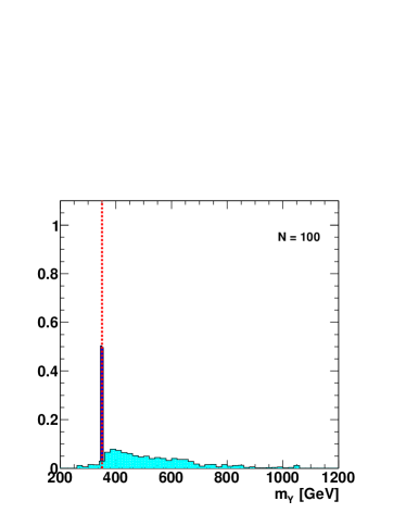
Figure 5: The distribution of winning mass hypotheses across pseudoexperiments using the phase space analysis (blue) and endpoint analysis (cyan) for the “2+2+2” topology. The true mass values in the benchmark spectrum used to generate the data are shown by dashed red lines.

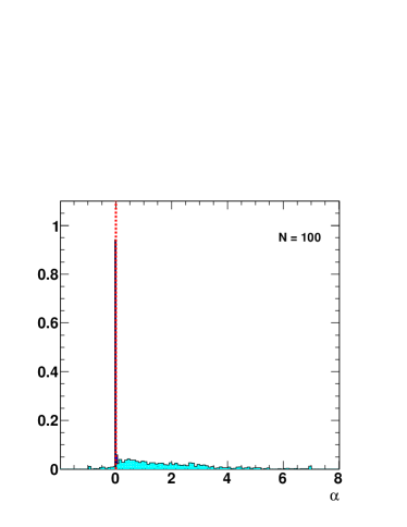
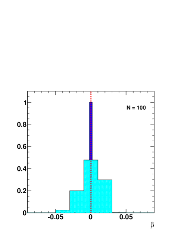
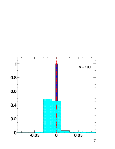
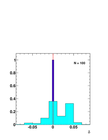
Figure 6: The distribution of winning mass hypotheses across pseudoexperiments using the phase space analysis (blue) and endpoint analysis (cyan) for the “2+2+2” topology in terms of $\{\alpha,\beta,\gamma,\delta\}$. The true mass values in the benchmark spectrum used to generate the data are shown by dashed red lines.

IV.2 The 2+3 Topology

For the 2+3 topology we choose to work with the benchmark spectrum

$$m_{X} =500\textrm{ GeV}\,,\qquad m_{Y}=350\textrm{ GeV}\,,\qquad m_{4}=100\textrm{ GeV}\,,$$

$$\qquad\qquad m_{1}=m_{2}=m_{3}=5\textrm{ GeV}\,.$$ (28)

which follows from the benchmark spectrum we used for the 2+2+2 topology by making $Z$ very heavy, so that it is always off-shell.

We use the following set of mass hypotheses for both the phase space and the endpoint analyses:

$$\tilde{m}_{\sigma}=M_{\sigma}+(100~{}{\rm GeV})\left(\alpha V_{\sigma}^{(1)}+\beta V_{\sigma}^{(2)}+\gamma V_{\sigma}^{(3)}\right)\qquad\sigma=\{X,Y,4\}\,,$$ (29)

where

$$V_{\sigma}^{(1)} =\{1,1,1\}$$

$$V_{\sigma}^{(2)} =\{0,1,-1\}$$

$$V_{\sigma}^{(3)} =\{2,-1,-1\}\,.$$ (30)

Once again, $V_{\sigma}^{(1)}$ corresponds to the flat direction. For the phase space analysis, we choose the scan

$$\alpha \in[-1,1] \Delta\alpha =0.01,$$

$$\beta \in[-0.1,0.1] \Delta\beta =0.005,$$

$$\gamma \in[-0.05,0.05] \Delta\gamma =0.0025\,.$$ (31)

As before, choices of $(\alpha,\beta,\gamma)$ are discarded for which the inequality $\tilde{m}_{X}>\tilde{m}_{Y}>\tilde{m}_{4}>0$ is violated. For the endpoint analysis, we scale this grid up by a factor of 2, since in this case a wider range of mass hypotheses can be picked as the winners.

As in the 2+2+2 topology, we run the phase space and endpoint analyses on a large number of pseudoexperiments of 100 events each. Furthermore, in order to study the robustness of our conclusions, we choose to run a parallel study, this time with 1000 events in each pseudoexperiment. In figures 7 and 8 we plot the distribution of winners in these two runs in both the $(\alpha,\beta,\gamma)$ and $\{\tilde{m}_{X},\tilde{m}_{Y},\tilde{m}_{4}\}$ parameterizations. The mean and standard deviations of the mass parameters in both runs are reported in table 2.

Once again, it is very easy to observe stark difference in sensitivity between the two analysis methods. As in the 2+2+2 topology, the phase space analysis can resolve the flat direction. Note that while the spread along the flat direction in the endpoint analysis does not appear as broad in this case as in the 2+2+2 topology, this is partly due to the fact that the analysis is biased towards lower values of $\tilde{m}_{\sigma}$ and thus the flat direction is cut off by the physical requirement that $\tilde{m}_{4}\geq 0$. This bias can be understood quantitatively, as discussed in detail in appendix C.

Mass (GeV)	$N_{events}=100$		$N_{events}=1000$
	Phase space	Endpoints	Phase space	Endpoints
$m_{X}$	$495.84\pm 11.95$	$434.32\pm 25.93$	$499.40\pm 0.96$	$463.32\pm 11.66$
$m_{Y}$	$345.69\pm 12.13$	$284.11\pm 28.48$	$349.39\pm 0.97$	$312.94\pm 12.08$
$m_{4}$	$96.86\pm 13.97$	$37.61\pm 27.45$	$99.56\pm 1.08$	$63.83\pm 11.91$
$\alpha$	$-0.039\pm 0.127$	$-0.647\pm 0.272$	$(-5.49\pm 9.97)\times 10^{-3}$	$-0.37\pm 0.12$
$\beta$	$-0.006\pm 0.013$	$-0.017\pm 0.020$	$(0.89\pm 1.05)\times 10^{-3}$	$(-4.4\pm 3.9)\times 10^{-3}$
$\gamma$	$-0.001\pm 0.005$	$-0.005\pm 0.012$	$(0.23\pm 0.38)\times 10^{-3}$	$(-0.2\pm 3.0)\times 10^{-3}$

Table 2: Mean and standard deviation of the distribution of winning mass hypotheses across all pseudoexperiments using the phase space and endpoint analyses for the 2+3 topology, for different sample sizes.

Since we have higher statistics in the $N_{events}=1000$ run, we refine our scan range for this case. For the phase space analysis, the scan parameters were

$$\alpha \in[-3.5\times 10^{-2},1.0\times 10^{-2}]\qquad\Delta\alpha=5\times 10^{-4},$$

$$\beta \in[-4.0\times 10^{-3},1.0\times 10^{-3}]\qquad\Delta\beta=2\times 10^{-4},$$

$$\gamma \in[-1.5\times 10^{-3},0.5\times 10^{-3}]\qquad\Delta\gamma=10^{-4}.$$ (32)

For the endpoint analysis, the corresponding numbers chosen were,

$$\alpha \in[-2.0,2.0] \Delta\alpha =0.02,$$

$$\beta \in[-4.0\times 10^{-2},4.0\times 10^{-2}] \Delta\beta =2\times 10^{-3},$$

$$\gamma \in[-2.0\times 10^{-2},2.0\times 10^{-2}] \Delta\gamma =10^{-3}.$$ (33)

Indeed, the endpoint analysis in this case gives a reasonable estimate of the masses, with a precision of less than $10\%$, and a smaller bias (within $\sim 3\sigma$ of the true value). In contrast, however, the endpoint analysis with $N_{events}=100$ gives very inaccurate results, whereas the phase space analysis still performs well. This makes it clear that while the phase space analysis is still preferred at high statistics due to reduced errors, it becomes indispensable at low statistics.

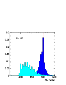
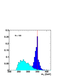
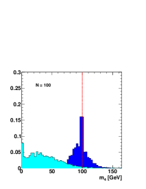
(a)

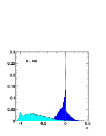
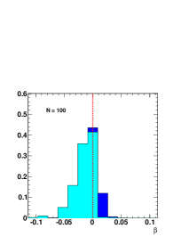
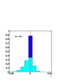
(b)

Figure 7: The distribution of winning mass hypotheses across pseudoexperiments with 100 events each using the phase space analysis (blue) and endpoint analysis (cyan) for the “2+3” topology, both in terms of the physical masses and also parameterized by $(\alpha,\beta,\gamma)$ as explained in the text. The true values in the benchmark spectrum used to generate the data are shown by dashed red lines. The sawtooth-like shape in the $m_{X}$ histogram is an artifact of the finite grid size.

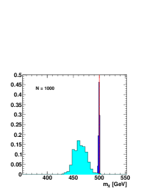
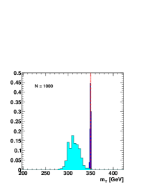
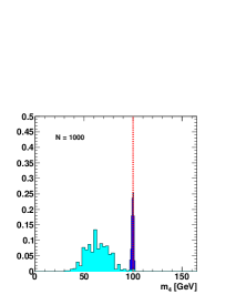
(a)

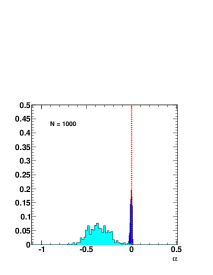
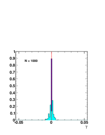
(b)

Figure 8: The distribution of winning mass hypotheses across pseudoexperiments with 1000 events each using the phase space analysis (blue) and endpoint analysis (cyan) for the “2+3” topology, both in terms of the physical masses and also parameterized by $(\alpha,\beta,\gamma)$ as explained in the text. The true values in the benchmark spectrum used to generate the data are shown by dashed red lines.

V Outlook and Conclusions

Given that the LHC has not already observed signs of new physics, there is a significant probability that even if we find new physics, we will have only a small number of signal events available to study its properties. We have demonstrated that in a low statistics environment, mass determination in cascade decays can be significantly improved by determining the boundary of the kinematically accessible phase space in its full dimensionality. This yields better results than traditional methods based on the presence of edges and endpoint in one-dimensional kinematic distributions because:

1. There are correlations in the distribution of events in the full phase space that are lost when the phase space is projected onto any one-dimensional observable.

2. For cascade decays with more than three final state particles, the phase space density is enhanced near the edge of the kinematically accessible region, allowing one to map the boundary with better resolution and utilize the aforementioned correlations.

By focusing on an event topology with one particle decaying to three visible and one invisible final state particle through a two-stage decay, we were able to demonstrate this improvement in mass determination quantitatively. Not only were the the best fit values for the unknown masses found to be closer to the true values used in the generation of the data, but the uncertainties in the measurement were also shown to be smaller when the analysis was performed on the full phase space in a likelihood-based analysis. Finally, while mass determination methods based on kinematic edges and endpoints exhibit a weakness in that they are sensitive to differences of masses in the spectrum but insensitive to the overall scale, the phase space analysis allows one to measure all unknown masses in the decay chain accurately.

While we demonstrated the applicability of our results on a reasonably simple event topology, our conclusions have wider applicability. The polynomial method may fail to apply even for a longer decay chains, if the cascade proceeds through three-body decays, in which case the system remains underconstrained. The phase space methods on the other hand become more powerful in this case since the shape of the phase space boundary in higher dimensions carries all the necessary information about the masses of the unknown particles occurring in the cascade. It should be noted however that the functional form of the phase space density is complicated for more than four final state particles and we leave the study of a more general class of decay topologies to future work.

In conclusion, we wish to briefly address future directions of study and also dwell on how the simplifying assumptions made in this study can be relaxed such that the validity of our conclusions can be tested in a more realistic collider analysis.

• The phase space analysis can be extended to cases where both sides of the event contain a cascade. The main added complication in this case is the inclusion of the additional constraint due to the measurement of the missing transverse energy (MET) into the analysis. This can be done in terms of Lorentz-invariant variables by introducing “reference” momenta (for example the four-momenta of the beams) which can be used in order to construct projection operators onto the transverse plane.

  For cascades on either side of the event which have fewer than four final state particles (one of which is invisible), there is at most one Lorentz invariant observable for that side of the event, thus it is not possible to go beyond an edge or endpoint analysis on either side alone. It is in these cases where it may be of interest to consider the full phase space distribution of the entire event, rather than each side of the event separately, which necessitates the inclusion of the MET constraint into the likelihood method. In the extreme case of only one visible final state on either side, there is only a single Lorentz invariant observable for the entire event. This is consistent with the conclusion of ref. Cheng and Han (2008) that a single variable, $m_{T2}$, captures all available information about the kinematics for this decay topology.

• While we have focused solely on the properties of the phase space density in this work, given a particular model, it is straightforward to incorporate the full matrix element for specific processes as well into the likelihood analysis as well. Such an analysis will not only differentiate between mass hypotheses, but it can also yield information about the spins and interactions of the particles involved.

• In our study, we have assumed an ideal detector with perfect energy resolution. As a result, even a single event that were incompatible with a given mass hypothesis could rule it out. In a study with a more realistic detector model, the effects of finite energy resolution will need to be taken into account. This can be accomplished by convoluting the likelihood with the response of the detector. The likelihood will then have a tail beyond the boundary of phase space. This will almost certainly reduce the precision of the mass measurement, however it should be kept in mind that a similar degradation will occur in the edge and endpoint based measurements as well.

• We have ignored the issue of combinatoric ambiguity. This can be particularly unrealistic when there are a large number of identical final states. The definition of the likelihood can be extended to sum over all possible ways that the observed particles can be assigned to the final state particles in the decay topology.

• We have assumed that the correct decay topology is used in the analysis. One can imagine relaxing this assumption without greatly modifying the analysis, by comparing the likelihoods based on a range of applicable decay topologies. This way, a likelihood analysis based on the full dimensionality of phase space can be used effectively not only to measure the masses of unknown particles but also to determine the correct underlying decay topology among a number of alternatives.

• We have ignored the presence of SM backgrounds in our study. In order to remove this assumption, one needs to model the background distribution in the multidimensional phase space and assign a likelihood to each event as having arisen from signal or from background based upon this model. Similar statistical techniques are used in likelihood-based analyses in new physics searches by ATLAS and CMS, though in a different context. It may in general be difficult to obtain an accurate model of the full background distribution, which will reduce the precision of the mass measurement. While a degradation will also occur as background is included in edge and endpoint based analyses, the degree to which the two analyses will be impacted is difficult to predict. On one hand, a multidimensional background model is more arbitrary and may therefore lead to greater loss of precision in the result of the mass measurement. On the other hand, due to the enhancement of the signal phase space distribution near the boundary of phase space, which is absent for the background, the details of the background model away from the boundary may not be as important as it would at first appear. One way to visualize this is to imagine an extreme limit where the signal events all lie on the boundary, while the background will vary smoothly in the direction orthogonal to the boundary, but the precise way in which the distribution of the background is modeled along this direction would not be important.

A more detailed study is necessary in order to more exactly quantify the impact of removing these simplifying assumptions on the precision of the mass measurements based on the likelihood based method vs. the edge and endpoint based methods. This will be further explored in future work.

Appendix A Formulae for edges and end-points

In this appendix we present the list of analytical formulae for the position of edges and endpoints in one-dimensional kinematic distributions that we use in our analysis. These have been well studied in the literature Hinchliffe et al. (1997); Allanach et al. (2000); Gjelsten et al. (2004, 2005); Miller et al. (2006); Burns et al. (2009b); Matchev et al. (2009). Throughout this section, we work in the approximation $m_{1}=m_{2}=m_{3}\simeq 0$. We have verified numerically that this approximation is valid for our purposes.

A.1 2+2+2 Topology

$$(m_{123}^{2})_{max} =\begin{cases}\frac{(m_{X}^{2}-m_{Y}^{2})(m_{Y}^{2}-m_{4}^{2})}{m_{Y}^{2}}&\frac{m_{X}}{m_{Y}}>\frac{m_{Y}}{m_{Z}}\frac{m_{Z}}{m_{4}}\\ \frac{(m_{X}^{2}m_{Z}^{2}-m_{Y}^{2}m_{4}^{2})(m_{Y}^{2}-m_{Z}^{2})}{m_{Y}^{2}m_{Z}^{2}}&\frac{m_{Y}}{m_{Z}}>\frac{m_{Z}}{m_{4}}\frac{m_{X}}{m_{Y}}\\ \frac{(m_{X}^{2}-m_{Z}^{2})(m_{Z}^{2}-m_{4}^{2})}{m_{Z}^{2}}&\frac{m_{Z}}{m_{4}}>\frac{m_{X}}{m_{Y}}\frac{m_{Y}}{m_{Z}}\\ (m_{X}-m_{4})^{2}&\mathrm{otherwise}\end{cases}$$ (34)

$$(m_{23}^{2})_{max} =(m_{Y}^{2}-m_{Z}^{2})(m_{Z}^{2}-m_{4}^{2})/m_{Z}^{2},$$ (35)

$$(m_{12}^{2})_{max} =(m_{X}^{2}-m_{Y}^{2})(m_{Y}^{2}-m_{Z}^{2})/m_{Y}^{2},$$ (36)

$$(m_{13}^{2})_{max} =(m_{X}^{2}-m_{Y}^{2})(m_{Z}^{2}-m_{4}^{2})/m_{Z}^{2}\,.$$ (37)

In cases where some of the final state particles are not distinguishable, it can be more convenient to use endpoints in the distribution of the higher and lower invariant mass of certain combinations of final states. For example, if the visible final states contain one lepton and two jets, the two possible lepton-jet pair invariant masses can be labeled event-by-event as $m^{2}_{lj,high}$ and $m^{2}_{lj,low}$, rather than $m^{2}_{lj_{1}}$ and $m^{2}_{lj_{2}}$. Since we assume that we can identify the final states, this issue does not arise in our study.

A.2 2+3 Topology

Since for the 2+3 Topology, there is no intrinsic distinction that sets particles 2 and 3 apart, the kinematic distributions respect the discrete symmetry $2\leftrightarrow 3$.

$$(m_{123}^{2})_{max} =\begin{cases}\frac{(m_{X}^{2}-m_{Y}^{2})(m_{Y}^{2}-m_{Z}^{2})}{m_{Y}^{2}}&\frac{m_{X}}{m_{Y}}>\frac{m_{Y}}{m_{4}}\\ (m_{X}-m_{4})^{2}&\mathrm{otherwise}\end{cases}$$ (38)

$$(m_{23}^{2})_{max} =(m_{Y}-m_{4})^{2},$$ (39)

$$(m_{12}^{2})_{max} =(m_{13}^{2})_{max}=(m_{X}^{2}-m_{Y}^{2})(m_{Y}^{2}-m_{4}^{2})/m_{Y}^{2}\,.$$ (40)

Appendix B $m_{34}^{2}$ Integral for the 2+3 Topology

In this appendix we provide additional details about how to analytically take the $m_{34}^{2}$ integration necessary for the likelihood analysis in the 2+3 topology. The integral is performed most easily by switching from the $m_{ij}^{2}$ variables to the set $\{m_{12},m_{23},m_{123},m_{34}\}$, which are linearly related to each other. In this basis, $\Delta_{4}$ is quadratic in $m_{34}^{2}$, and can be therefore written as

$$\Delta_{4} =\frac{1}{16}(am_{34}^{4}+bm_{34}^{2}+c),$$

$$=\frac{1}{16}a(m_{34}^{2}-s_{34}^{+})(m_{34}^{2}-s_{34}^{-}),$$ (41)

where,

$$s_{34}^{\pm}=-\frac{b}{2a}\pm\frac{\sqrt{b^{2}-4ac}}{2a}.$$ (42)

Since $\Delta_{4}>0$ defines the physical phase-space region, $s_{34}^{\pm}$ determine the range of the $m_{34}^{2}$ integration.

The constants $a$ and $b$ appearing above are,

$$a =\lambda\left(m_{1}^{2},m_{23}^{2},m_{123}^{2}\right),$$ (43)

$$b =2\ \mathrm{Det}\left|\begin{array}[]{ccc}2m_{23}^{2}&m_{123}^{2}+m_{23}^{2}-m_{1}^{2}&m_{23}^{2}-m_{Y}^{2}+m_{4}^{2}\\ m_{123}^{2}+m_{23}^{2}-m_{1}^{2}&2m_{123}^{2}&m_{123}^{2}-m_{X}^{2}+m_{4}^{2}\\ m_{23}^{2}-m_{2}^{2}+m_{3}^{2}&m_{123}^{2}-m_{12}^{2}+m_{3}^{2}&m_{3}^{2}+m_{4}^{2}\end{array}\right|,$$ (47)

$$b^{2}-4ac =16\ G\left(m_{12}^{2},m_{23}^{2},m_{123}^{2},m_{2}^{2},m_{1}^{2},m_{3}^{2}\right)G\left(m_{123}^{2},m_{Y}^{2},m_{X}^{2},m_{23}^{2},m_{1}^{2},m_{4}^{2}\right),$$ (48)

where the kinematic functions $\lambda$ and $G$ were defined in equation 20.

Using this expression for $\Delta_{4}$ quadratic in $m_{34}^{2}$ it is not too difficult to verify that equation 16 follows from equation 15.

Appendix C Understanding the edge/end-point results

This appendix is devoted to interpreting the performance of the endpoint analysis, and in particular its insensitivity along the flat direction parametrized by one parameter, say $\tilde{m}_{4}$ with the other masses chosen as $\tilde{m}_{\sigma}-\tilde{m}_{4}=M_{\sigma}-M_{4}$ where $M_{\sigma}$ correspond to the true mass point used to generate the data. Understanding this flat direction will also provide insight on the bias in the mass measurement that we observe in the endpoint analysis. In this appendix we will study the flat direction for the specific analysis that we describe in the main body of the paper but for a more general understanding of the flat direction the reader is also encouraged to consult references Cho et al. (2008a); Gripaios (2008); Cho et al. (2008c); Barr et al. (2008b, 2009b); Burns et al. (2009a, b).

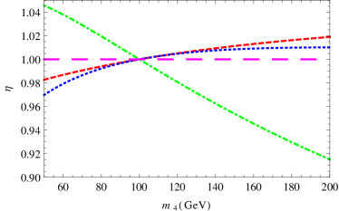
(a)

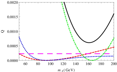
(b)

Figure 9: a) Ratio of predicted values (based on a mass hypothesis along the flat direction) to the true values of the endpoints in $m^{2}_{12}$ (red, dashed), $m^{2}_{23}$ (blue, dotted), $m^{2}_{13}$ (green, dot-dashed) and $m^{2}_{123}$ (magenta, long-dashed) in the 2+2+2 topology. b) The quality-of-fit variable (defined in equation 14) for each endpoint along the flat direction. A representative pseudoexperiment is chosen for illustration. The solid black curve corresponds to the total quality-of-fit variable $Q$ for the same pseudoexperiment.

C.1 2+2+2 Topology

In order to estimate the dependence of various edge positions along the flat direction, we plot the ratio of the predicted endpoint position as calculated with hypothetical masses to the true endpoint position, as a function of $\tilde{m}_{4}$. As can be seen from Figure 9, the endpoints are relatively insensitive to variation of masses along this direction. In fact, the mass measurement is driven by $(m_{13}^{2})_{max}$.

Moreover, in a low statistics sample, kinematic distributions are often not well populated at the maximal allowed values. This is especially the case for endpoints (rather than edges), where the approach to the maximal value is rather shallow. We use a representative pseudoexperiment to investigate this effect quantitatively. From figure 9, it is clear that a lower value for $m^{2}_{13}$ biases the winning hypothesis towards higher values of $m_{4}$. This has the effect of pushing the entire best fit spectrum to higher values.

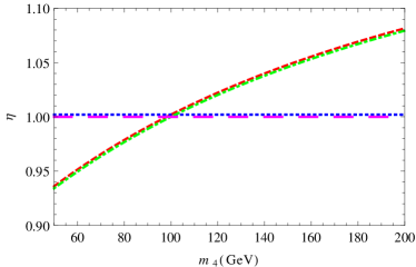
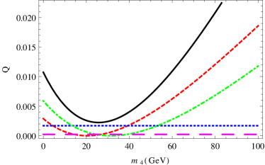
Figure 10: a) Ratio of predicted values (based on a mass hypothesis along the flat direction) to the true values of the endpoints in $m^{2}_{12}$ (red, dashed), $m^{2}_{23}$ (blue, dotted), $m^{2}_{13}$ (green, dot-dashed) and $m^{2}_{123}$ (magenta, long-dashed) in the 2+3 topology. b) The quality-of-fit variable (defined in equation 14) for each endpoint along the flat direction. A representative pseudoexperiment is chosen for illustration. The solid black curve corresponds to the total quality-of-fit variable $Q$ for the pseudoexperiment.

C.2 2+3 Topology

We also study the effect of the flat direction for the 2+3 topology. In this case, the kinematic distributions have only endpoints but no edges which are poorly populated, especially at low statistics.

As for the 2+2+2 topology, we plot the true value of endpoints in figure 10 for each kinematic distribution and compare them with the predicted endpoints for the hypothetical masses, varied along the flat direction. A representative pseudoexperiment is again chosen to illustrate the point. We see that $(m^{2}_{23})_{max}$ and $(m^{2}_{31})_{max}$ are the only endpoints which are sensitive along this direction, and consequently they drive the mass measurement.

Since these two distributions have relatively shallow tails, the measured endpoint of a low statistics sample falls fairly short of the true endpoint, leading to a large bias in the mass measurement. From figure 10, it is clear that the bias is towards smaller masses in this case.

References

- Beenakker et al. (1998) W. Beenakker, M. Kramer, T. Plehn, M. Spira, and P. Zerwas, Nucl.Phys. B515, 3 (1998), eprint hep-ph/9710451.
- Beenakker et al. (1999) W. Beenakker, M. Klasen, M. Kramer, T. Plehn, M. Spira, et al., Phys.Rev.Lett. 83, 3780 (1999), eprint hep-ph/9906298.
- Hinchliffe et al. (1997) I. Hinchliffe, F. Paige, M. Shapiro, J. Soderqvist, and W. Yao, Phys.Rev. D55, 5520 (1997), eprint hep-ph/9610544.
- Bachacou et al. (2000) H. Bachacou, I. Hinchliffe, and F. E. Paige, Phys.Rev. D62, 015009 (2000), eprint hep-ph/9907518.
- Allanach et al. (2000) B. Allanach, C. Lester, M. A. Parker, and B. Webber, JHEP 0009, 004 (2000), eprint hep-ph/0007009.
- Lester (2001) C. G. Lester, Ph.D. thesis, University of Cambridge (2001).
- Gjelsten et al. (2004) B. Gjelsten, . Miller, D.J., and P. Osland, JHEP 0412, 003 (2004), eprint hep-ph/0410303.
- Gjelsten et al. (2005) B. Gjelsten, . Miller, D.J., and P. Osland, JHEP 0506, 015 (2005), eprint hep-ph/0501033.
- Lester et al. (2006) C. G. Lester, M. A. Parker, and M. J. White, JHEP 0601, 080 (2006), eprint hep-ph/0508143.
- Miller et al. (2006) . Miller, D.J., P. Osland, and A. Raklev, JHEP 0603, 034 (2006), eprint hep-ph/0510356.
- Lester (2007) C. G. Lester, Phys.Lett. B655, 39 (2007), eprint hep-ph/0603171.
- Ross and Serna (2008) G. G. Ross and M. Serna, Phys.Lett. B665, 212 (2008), eprint 0712.0943.
- Tovey (2008) D. R. Tovey, JHEP 0804, 034 (2008), eprint 0802.2879.
- Barr et al. (2008a) A. J. Barr, G. G. Ross, and M. Serna, Phys.Rev. D78, 056006 (2008a), eprint 0806.3224.
- Barr et al. (2009a) A. J. Barr, A. Pinder, and M. Serna, Phys.Rev. D79, 074005 (2009a), eprint 0811.2138.
- Webber (2009) B. Webber, JHEP 0909, 124 (2009), eprint 0907.5307.
- Hinchliffe and Paige (1999) I. Hinchliffe and F. Paige, Phys.Rev. D60, 095002 (1999), eprint hep-ph/9812233.
- Nojiri et al. (2003) M. Nojiri, G. Polesello, and D. Tovey (2003), eprint hep-ph/0312317.
- Kawagoe et al. (2005) K. Kawagoe, M. Nojiri, and G. Polesello, Phys.Rev. D71, 035008 (2005), eprint hep-ph/0410160.
- Gjelsten et al. (2006) B. Gjelsten, . Miller, D.J., P. Osland, and A. Raklev, Conf.Proc. C060726, 1171 (2006), eprint hep-ph/0611080.
- Cheng et al. (2007) H.-C. Cheng, J. F. Gunion, Z. Han, G. Marandella, and B. McElrath, JHEP 0712, 076 (2007), eprint 0707.0030.
- Nojiri and Takeuchi (2008) M. M. Nojiri and M. Takeuchi, JHEP 0810, 025 (2008), eprint 0802.4142.
- Cheng et al. (2008) H.-C. Cheng, D. Engelhardt, J. F. Gunion, Z. Han, and B. McElrath, Phys.Rev.Lett. 100, 252001 (2008), eprint 0802.4290.
- Cheng et al. (2009) H.-C. Cheng, J. F. Gunion, Z. Han, and B. McElrath, Phys.Rev. D80, 035020 (2009), eprint 0905.1344.
- Matchev et al. (2009) K. T. Matchev, F. Moortgat, L. Pape, and M. Park, JHEP 0908, 104 (2009), eprint 0906.2417.
- Autermann et al. (2009) C. Autermann, B. Mura, C. Sander, H. Schettler, and P. Schleper (2009), eprint 0911.2607.
- Kim (2010) I.-W. Kim, Phys.Rev.Lett. 104, 081601 (2010), eprint 0910.1149.
- Han et al. (2010) T. Han, I.-W. Kim, and J. Song, Phys.Lett. B693, 575 (2010), eprint 0906.5009.
- Kang et al. (2010a) Z. Kang, N. Kersting, S. Kraml, A. Raklev, and M. White, Eur.Phys.J. C70, 271 (2010a), eprint 0908.1550.
- Nojiri et al. (2010) M. M. Nojiri, K. Sakurai, and B. R. Webber, JHEP 1006, 069 (2010), eprint 1005.2532.
- Kang et al. (2010b) Z. Kang, N. Kersting, and M. White (2010b), eprint 1007.0382.
- Hubisz and Shao (2011) J. Hubisz and J. Shao, Phys.Rev. D84, 035031 (2011), eprint 1009.1148.
- Cheng et al. (2010) H.-C. Cheng, Z. Han, I.-W. Kim, and L.-T. Wang, JHEP 1011, 122 (2010), eprint 1008.0405.
- Gripaios et al. (2011) B. Gripaios, K. Sakurai, and B. Webber, JHEP 1109, 140 (2011), eprint 1103.3438.
- Han et al. (2013a) T. Han, I.-W. Kim, and J. Song, Phys.Rev. D87, 035003 (2013a), eprint 1206.5633.
- Han et al. (2013b) T. Han, I.-W. Kim, and J. Song, Phys.Rev. D87, 035004 (2013b), eprint 1206.5641.
- Lester and Summers (1999) C. Lester and D. Summers, Phys.Lett. B463, 99 (1999), eprint hep-ph/9906349.
- Barr et al. (2003) A. Barr, C. Lester, and P. Stephens, J.Phys. G29, 2343 (2003), eprint hep-ph/0304226.
- Meade and Reece (2006) P. Meade and M. Reece, Phys.Rev. D74, 015010 (2006), eprint hep-ph/0601124.
- Baumgart et al. (2007) M. Baumgart, T. Hartman, C. Kilic, and L.-T. Wang, JHEP 0711, 084 (2007), eprint hep-ph/0608172.
- Matsumoto et al. (2007) S. Matsumoto, M. M. Nojiri, and D. Nomura, Phys.Rev. D75, 055006 (2007), eprint hep-ph/0612249.
- Lester and Barr (2007) C. Lester and A. Barr, JHEP 0712, 102 (2007), eprint 0708.1028.
- Cho et al. (2008a) W. S. Cho, K. Choi, Y. G. Kim, and C. B. Park, Phys.Rev.Lett. 100, 171801 (2008a), eprint 0709.0288.
- Gripaios (2008) B. Gripaios, JHEP 0802, 053 (2008), eprint 0709.2740.
- Nojiri et al. (2008a) M. M. Nojiri, Y. Shimizu, S. Okada, and K. Kawagoe, JHEP 0806, 035 (2008a), eprint 0802.2412.
- Cho et al. (2008b) W. S. Cho, K. Choi, Y. G. Kim, and C. B. Park, Phys.Rev. D78, 034019 (2008b), eprint 0804.2185.
- Serna (2008) M. Serna, JHEP 0806, 004 (2008), eprint 0804.3344.
- Nojiri et al. (2008b) M. M. Nojiri, K. Sakurai, Y. Shimizu, and M. Takeuchi, JHEP 0810, 100 (2008b), eprint 0808.1094.
- Cho et al. (2009a) W. S. Cho, K. Choi, Y. G. Kim, and C. B. Park, Phys.Rev. D79, 031701 (2009a), eprint 0810.4853.
- Cheng and Han (2008) H.-C. Cheng and Z. Han, JHEP 0812, 063 (2008), eprint 0810.5178.
- Choi et al. (2009) K. Choi, S. Choi, J. S. Lee, and C. B. Park, Phys.Rev. D80, 073010 (2009), eprint 0908.0079.
- Matchev and Park (2011) K. T. Matchev and M. Park, Phys.Rev.Lett. 107, 061801 (2011), eprint 0910.1584.
- Cohen et al. (2010) T. Cohen, E. Kuflik, and K. M. Zurek, JHEP 1011, 008 (2010), eprint 1003.2204.
- Polesello and Tovey (2010) G. Polesello and D. R. Tovey, JHEP 1003, 030 (2010), eprint 0910.0174.
- Konar et al. (2010a) P. Konar, K. Kong, K. T. Matchev, and M. Park, Phys.Rev.Lett. 105, 051802 (2010a), eprint 0910.3679.
- Konar et al. (2010b) P. Konar, K. Kong, K. T. Matchev, and M. Park, JHEP 1004, 086 (2010b), eprint 0911.4126.
- Curtin (2012) D. Curtin, Phys.Rev. D85, 075004 (2012), eprint 1112.1095.
- Nojiri and Sakurai (2010) M. M. Nojiri and K. Sakurai, Phys.Rev. D82, 115026 (2010), eprint 1008.1813.
- Lester (2011) C. G. Lester, JHEP 1105, 076 (2011), eprint 1103.5682.
- Mahbubani et al. (2013) R. Mahbubani, K. T. Matchev, and M. Park, JHEP 1303, 134 (2013), eprint 1212.1720.
- Agashe et al. (2013a) K. Agashe, R. Franceschini, and D. Kim, Phys.Rev. D88, 057701 (2013a), eprint 1209.0772.
- Agashe et al. (2013b) K. Agashe, R. Franceschini, and D. Kim (2013b), eprint 1309.4776.
- Kondo (1988) K. Kondo, J.Phys.Soc.Jap. 57, 4126 (1988).
- Dalitz and Goldstein (1992) R. Dalitz and G. R. Goldstein, Phys.Rev. D45, 1531 (1992).
- Abazov et al. (2004) V. Abazov et al. (D0 Collaboration), Nature 429, 638 (2004), eprint hep-ex/0406031.
- Artoisenet et al. (2010) P. Artoisenet, V. Lemaitre, F. Maltoni, and O. Mattelaer, JHEP 1012, 068 (2010), eprint 1007.3300.
- Alwall et al. (2011a) J. Alwall, A. Freitas, and O. Mattelaer, Phys.Rev. D83, 074010 (2011a), eprint 1010.2263.
- Fiedler et al. (2010) F. Fiedler, A. Grohsjean, P. Haefner, and P. Schieferdecker, Nucl.Instrum.Meth. A624, 203 (2010), eprint 1003.1316.
- Gainer et al. (2013) J. S. Gainer, J. Lykken, K. T. Matchev, S. Mrenna, and M. Park (2013), eprint 1307.3546.
- Alwall et al. (2010) J. Alwall, A. Freitas, and O. Mattelaer, AIP Conf.Proc. 1200, 442 (2010), eprint 0910.2522.
- Cho et al. (2008c) W. S. Cho, K. Choi, Y. G. Kim, and C. B. Park, JHEP 0802, 035 (2008c), eprint 0711.4526.
- Barr et al. (2008b) A. J. Barr, B. Gripaios, and C. G. Lester, JHEP 0802, 014 (2008b), eprint 0711.4008.
- Barr et al. (2009b) A. J. Barr, B. Gripaios, and C. G. Lester, JHEP 0911, 096 (2009b), eprint 0908.3779.
- Burns et al. (2009a) M. Burns, K. Kong, K. T. Matchev, and M. Park, JHEP 0903, 143 (2009a), eprint 0810.5576.
- Burns et al. (2009b) M. Burns, K. T. Matchev, and M. Park, JHEP 0905, 094 (2009b), eprint 0903.4371.
- Cho et al. (2009b) W. Cho, K. Choi, Y. Kim, and C. Park, AIP Conf.Proc. 1078, 274 (2009b).
- Arkani-Hamed and Dimopoulos (2005) N. Arkani-Hamed and S. Dimopoulos, JHEP 0506, 073 (2005), eprint hep-th/0405159.
- Giudice and Romanino (2004) G. Giudice and A. Romanino, Nucl.Phys. B699, 65 (2004), eprint hep-ph/0406088.
- Arkani-Hamed et al. (2005) N. Arkani-Hamed, S. Dimopoulos, G. Giudice, and A. Romanino, Nucl.Phys. B709, 3 (2005), eprint hep-ph/0409232.
- Arkani-Hamed et al. (2012) N. Arkani-Hamed, A. Gupta, D. E. Kaplan, N. Weiner, and T. Zorawski (2012), eprint 1212.6971.
- Bai and Cheng (2011) Y. Bai and H.-C. Cheng, JHEP 1106, 021 (2011), eprint 1012.1863.
- Birkedal et al. (2005) A. Birkedal, R. Group, and K. Matchev, eConf C050318, 0210 (2005), eprint hep-ph/0507002.
- Costanzo and Tovey (2009) D. Costanzo and D. R. Tovey, JHEP 0904, 084 (2009), eprint 0902.2331.
- Rajaraman and Yu (2011) A. Rajaraman and F. Yu, Phys.Lett. B700, 126 (2011), eprint 1009.2751.
- Baringer et al. (2011) P. Baringer, K. Kong, M. McCaskey, and D. Noonan, JHEP 1110, 101 (2011), eprint 1109.1563.
- Choi et al. (2011) K. Choi, D. Guadagnoli, and C. B. Park, JHEP 1111, 117 (2011), eprint 1109.2201.
- Byers and Yang (1964) N. Byers and C. N. Yang, Rev. Mod. Phys. 36, 595 (1964), URL http://link.aps.org/doi/10.1103/RevModPhys.36.595.
- Byckling and Kajantie (1973) E. Byckling and K. Kajantie, Particle Kinematics (John Wiley & Sons Ltd, 1973), ISBN 9780471128854.
- Alwall et al. (2011b) J. Alwall, M. Herquet, F. Maltoni, O. Mattelaer, and T. Stelzer, JHEP 1106, 128 (2011b), eprint 1106.0522.