The Main Sequence of three Red Supergiant Clusters

Abstract

Massive clusters in our Galaxy are an ideal testbed to investigate the properties and evolution of high mass stars. They provide statistically significant samples of massive stars of uniform ages. To accurately determine the intrinsic physical properties of these stars we need to establish the distances, ages and reddening of the clusters. One avenue to achieve this is the identification and characterisation of the main sequence members of red supergiant rich clusters.

Here we utilise publicly available data from the UKIDSS galactic plane survey. We show that point spread function photometry in conjunction with standard photometric decontamination techniques allows us to identify the most likely main sequence members in the 10-20 Myr old clusters RSGC 1, 2, and 3. We confirm the previous detection of the main sequence in RSGC 2 and provide the first main sequence detection in RSGC 1 and RSGC 3. There are in excess of 100 stars with more than 8 $M_{\odot}$ identified in each cluster. These main sequence members are concentrated towards the spectroscopically confirmed red supergiant stars. We utilise the $J$$-$$K$ colours of the bright main sequence stars to determine the $K$-band extinction towards the clusters. The differential reddening is three times as large in the youngest cluster RSGC 1 compared to the two older clusters RSGC 2 and RSGC 3. Spectroscopic follow up of the cluster main sequence stars should lead to more precise distance and age estimates for these clusters as well as the determination of the stellar mass function in these high mass environments.

1 Introduction

Massive stars are most commonly formed in clusters and associations (Gvaramadze et al., 2012), even if there are potential exceptions (e.g. Oey et al. (2013)). These building blocks are the sole observational characteristic of star formation that is observable in more distant galaxies. It is thus of importance to investigate the details of such massive clusters locally in our own Galaxy.

The identification of local examples of clusters and associations of massive stars is complicated by a number of facts. Such objects are generally rare in the Milky Way and are thus typically at large distances. The Sun’s position near the Galactic Plane, hence makes it difficult to identify and investigate these objects due to the large amounts of extinction along the line of sight. Furthermore, most massive star formation is projected towards the general direction of the Galactic Centre, which causes additional difficulties due to crowding.

Thus, the identification and characterisation of massive star clusters in our own Galaxy has only recently gained considerable momentum due to advances in infrared astronomy that allow us to probe these distant and obscured objects. Many of them have been known for a considerable time, but have not been recognised as massive star clusters. For example Westerlund 1 was discovered by Westerlund (1961) but only recognised as young, very massive cluster more than 30 yrs later (Clark et al., 1998; Piatti et al., 1998). Similarly, the cluster Stephenson 2 (Stephenson, 1990) had been known for many years until its true nature as Red Supergiant Cluster 2 (RSGC 2) was uncovered (Ortolani et al., 2002; Davies et al., 2007). Further, more systematic searches to uncover the population of the most massive clustes in the Galaxy are ongoing, e.g. Rahman et al. (2013).

Clusters at the top end of the mass distribution in our Galaxy (above $10^{4}$ M$\odot$) have, depending on their age, a sizable number of evolved massive stars. These are either Wolf-Rayet stars, or blue/yellow/red supergiants. There are now a number of galactic clusters with a large population of Red Supergiant (RSG) stars known, many of which are in a region confined to where the Scutum spiral arm meets the near side of the Galactic Bar. These are e.g. RSGC 1 to RSGC 5 (Figer et al., 2006; Davies et al., 2007; Clark et al., 2009; Alexander et al., 2009; Negueruela et al., 2010; Negueruela et al., 2011). All these clusters are about 6 kpc from the Sun, highly extincted, between 7 Myr and 20 Myr old and have masses in excess of 10.000 $M_{\odot}$. These clusters are thus an ideal testbed to study the formation and evolution of massive stars as well as their influence on the environment in great detail. However, it is important in the context of understanding the formation and evolution of massive clusters to investigate the distribution and properties of the lower mass stars as well as the bright supergiants and Wolf Rayet stars. In particular since the intrinsic properties of lower mass stars are much better understood, this should enable us to determine the distances, ages and reddening of these clusters more accurately.

The main sequence (MS) stars of these clusters have so far, however, not been investigated (though the slightly less massive and less reddened cluster NGC 7419 has recently been studied by Marco & Negueruela (2013)). Given that the RSG cluster members have an apparent brightness of about $K$ = 6 mag, one would expect to detect the MS in deep near-infrared (NIR) images, in particular the Galactic Plane Survey (GPS, Lucas et al. (2008)) data from the UK Deep Sky Survey (UKIDSS, Lawrence et al. (2007)) seems to be ideal to detect the fainter members of the RSG clusters mentioned above. But even data from the 2–Micron All Sky Survey (2MASS, Skrutskie et al. (2006)) should be deep enough to detect the brightest main sequence stars in these clusters.

Only for the cluster RSGC 2 has the main sequence been detected so far (Froebrich, 2013). The author uses 2MASS and GPS data to identify the top of the MS at colours of about $J$$-$$K$ = 1.5 mag and at a brightness of slightly fainter than $K$ = 10 mag. The author also investigates the data for RSGC 1 and RSGC 3 with the same methods but is unable to detect the main sequence for these clusters. It is speculated that this is caused by problems with accurate aperture photometry in the vicinity of the bright RSG stars in those objects. The main sequence in RSGC 2 is the easiest to detect due to the spatial extent of the cluster, which is the largest amongst the RSG clusters. Here we hence try to identify the main sequences of other known and candidate RSG clusters by means of point spread function (PSF) photometry in the JHK images of the UKIDSS GPS data. This will include some of the new RSG cluster candidates (F 3 and F 4) identified by (Froebrich, 2013) based on colour selected star density maps from 2MASS.

This paper is structured as follows. In Sect. 2 we briefly outline the data and analysis methods employed. We then discuss our results in Sect. 3 with focus on the properties of the main sequences detected in RSGC 1, 2, 3.

Table 1: Here we list the clusters and candidates investigated and their central coordinates. We also indicate the total number of stars in the 10′ $\times$ 10′ field around each cluster position in our input catalogue and the number of stars with good PSF photometry in all three bands that are brighter than the completeness limit in each filter (see text for details). We also list the $rms$ scatter of the photometric calibration of our PSF photometry into the UKIDSS system. The $min$ and $max$ columns give the range of magnitudes for which the calibration was performed. The $\sigma$ values denote the $rms$ scatter for each field, filter and specified magnitude range.

Field	RA	DEC	Number of stars		$J_{min}$	$J_{max}$	$\sigma_{J}$	$H_{min}$	$H_{max}$	$\sigma_{H}$	$K_{min}$	$K_{max}$	$\sigma_{K}$
	[deg] (J2000)		Input	Output	[mag]	[mag]	[mag]	[mag]	[mag]	[mag]	[mag]	[mag]	[mag]
RSGC 1	279.488	$-$6.880	31562	11976	14.0	17.0	0.024	13.0	16.0	0.034	12.0	15.0	0.045
RSGC 2	279.838	$-$6.029	42313	17872	13.0	16.0	0.021	12.0	15.0	0.024	11.0	14.0	0.028
RSGC 3	281.350	$-$3.387	43557	20960	13.0	16.0	0.021	12.0	15.0	0.026	12.0	15.0	0.046
F 3	274.910	$-$14.340	34837	15312	13.0	16.0	0.022	12.5	15.0	0.027	12.0	15.0	0.045
F 4	276.030	$-$13.330	43445	19664	13.0	16.0	0.036	12.0	15.0	0.029	11.0	14.0	0.035

2 Data and Analysis Methods

2.1 UKIDSS data

In Froebrich (2013) the main sequence of RSGC 2 has been detected in aperture photometry of UKIDSS GPS data between $K$ = 11 mag and $K$ = 14.5 mag. All stars brighter than this are saturated. Tentatively, this main sequence was also visible in 2MASS data starting from about $K$ = 10 mag. The red supergiants in this cluster are between 5^th and 6^th magnitude in the $K$-band (Davies et al., 2007). Thus, the brightest main sequence members in this cluster are five or six magnitudes fainter than the red supergiants. Given that several of the other known RSG clusters are in a similar position on the sky and potentially have similar ages, distances and reddening (Figer et al. (2006), Davies et al. (2007), Davies et al. (2008), Clark et al. (2009), Alexander et al. (2009)) one can assume that their main sequences should have analogue properties, i.e. should have similarly bright members. However, for none of the other investigated RSG clusters or candidates in Froebrich (2013) has the main sequence been detected in the GPS aperture photomety data. This was attributed to crowding in the clusters, and thus low quality aperture photometry of potential main sequence stars in the vicinity of the bright RSG cluster members. In other words, the GPS aperture photometry catalogue is highly incomplete near the bright RSG cluster stars. We hence selected RSGC 1 – 5 and the cluster candidates F 3 and F 4 from Froebrich (2013) for further investigations, i.e. PSF-photometry, to reveal their main sequences.

We downloaded 10′ $\times$ 10′ cut-outs of the JHK images from the UKIDSS GPS around the nominal position of each of these clusters via the Widefield Camera Science Archive webpage. We further obtained a complete list of all source detections (independent of the photometric quality) in each field. Typically there are about 30 – 45,000 detections in each of the fields. We then manually removed all detections which were obvious image artefacts (detector cross talk, persistence, etc.) and added all visible real stars missed by the source detection software to these catalogues. In particular near the bright red supergiant cluster members a number of real stars is missing. Several hundred detections have been removed/added for each field by visually inspecting the $K$-band images and manually deleting all obvious false detections and appending every object that has the appearance of a star but was missing in the photometric catalogue. In Table 1 we list the number of objects in these input catalogues for each cluster field.

2.2 PSF Photometry

We performed PSF fitting photometry in each image at all positions from the above generated input catalogue. For this purpose, we used the standard routines from DAOPHOT, as implemented in IRAF (Stetson, 1987). To define the PSF for a given frame, about 10 – 15 isolated reference stars distributed across the images were selected. Since the crowding was significant near the field center, most of these reference stars are located in the outskirts of the clusters. We did not notice any sign of a spatially varying PSF. The average PSF of these reference stars is modelled in DAOPHOT with a combination of an analytical function and an empirical image, which better represents the wings of the PSF. This model PSF was then fit to all objects in the catalogue, to create the final list of magnitudes. As measured by the $\chi^{2}$ and the PSF subtracted images, the PSF fitting performs well in the UKIDSS GPS images. Only in one case, the $K$-band image of the cluster candidate F 3, is the PSF undersampled and larger residuals are visible in the PSF subtracted images. However, the quality of the photometry is not significantly degraded in this image (see Table 1).

We merged the photometric catalogues for each of the JHK filters and used the GPS aperture photometry of sources in each field to calibrate the instrumental magnitudes. Only objects with pstar $\geq$ 0.99965 (see Lucas et al. (2008) for details on how this is defined) are used in the calibration and a nominal shift of the magnitudes and no colour terms are considered. The root mean square (rms) scatter of the calibrated magnitudes is listed in Table 1 together with the magnitude range in which the calibration was performed. There are some images where we detect a clear non-linearity for bright sources. This is expected, since the PSF fitting should be reliable over a wider range of the nonlinear regime. Thus, the colours and magnitudes for the bright stars could be systematically off. Note that this only influences the very top of the potential cluster main sequences and will have no influence on our analysis.

All point sources which did lack a detection by the PSF fitting routine in at least one of the three NIR bands were removed from the final catalogues. We also removed all stars which were fainter than the completeness limit (determined as the peak in the magnitude distribution) in at least one filter. Finally all objects that had a photometric uncertainty which differed by more than 2 $\sigma$ from the average of stars with the same apparent magnitude were removed. The number of stars in this output catalogue for each cluster is listed in Table 1.

2.3 Photometric Decontamination

Using the calibrated JHK PSF-photometry we performed a photometric decontamination of the stars in the cluster field to establish which stars are the most likely cluster members. The method is based on the technique described in Bonatto & Bica (2007) and references therein. It uses the $J$-band magnitudes and $J$$-$$H$ and $J$$-$$K$ colours to distinguish field stars from cluster members based on their apparent magnitudes and colours. This particular choice of colours provides the maximum variance among stellar cluster’s colour-magnitude sequences for open clusters of various ages (Bonatto et al., 2004; Bonatto & Bica, 2007). We use a slight adaptation of this method, outlined in detail in Froebrich et al. (2010). For each cluster we define as cluster area everything closer than the radius ($r$, as specified in Table 2) around the nominal cluster centre. Note that the radii for the clusters are based either on literature estimates or are chosen by us to include most of the confirmed or suspected RSG stars in each object. The actual value of the radius will not influence our conclusions. As control field we use all objects within the entire 10′ $\times$ 10′ field but further away than two cluster radii from the centre of the cluster. See Fig. B1 in the Appendix for a $K$-band and Glimpse 8 $\mu$m image of RSGC 1, 2, 3 with circles indicating the cluster and control fields. We also show the $J$ $-$ $K$ vs $K$ colour magnitude diagrams of the cluster and control fields for these clusters in Fig. C1 in the Appendix. For each star ($i$) in the cluster field we then determine the colour-colour-magnitude distance ($r_{ccm}$) to every other star ($j$) in the cluster field as:

$$r_{ccm}=\sqrt{\frac{1}{2}\left(J_{i}-J_{j}\right)^{2}+\left(JK_{i}-JK_{j}\right)^{2}+\left(JH_{i}-JH_{j}\right)^{2}}$$ (1)

Where $JK=J-K$ and $JH=J-H$ are the above mentioned near infrared colours. The $r_{ccm}$ distance in which there are 20 stars in the cluster area is denoted as $r^{20}_{ccm}$. It essentially defines the local density of stars in the near infrared colour-colour-magnitude space. Note that the specific choice of 20 stars does not influence any of our results and is a compromise between the accuracy of the membership probabilities (see below) and the ’resolution’ at which we can determine the position of the main sequence. We then determine the number of stars ($N^{con}_{ccm}$) at the same position and within the same radius of the colour-colour-magnitude space but for the stars in the control field. With this number, as well as the respective surface area of the control field ($A_{con}$) and cluster area ($A_{cl}$), we can determine the membership-likelihood index or cluster membership probability ($P^{i}_{cl}$) of the star $i$ as:

$$P^{i}_{cl}=1.0-\frac{N^{con}_{ccm}}{20}\frac{A_{cl}}{A_{con}}.$$ (2)

Note that these cluster membership probabilities are strictly speaking not real probabilities (Buckner & Froebrich 2013, subm.), since fluctuations of the field star density in principle allow negative values for $P^{i}_{cl}$. If this occurs in our analysis the $P^{i}_{cl}$ value is set to zero. However, the sum of all $P^{i}_{cl}$ values equals the excess number of stars in the cluster area compared to the control field. High values of $P^{i}_{cl}$ identify the stars in the cluster field which are the most likely members and thus allow us to establish the overall population of cluster stars statistically. Typically this method identifies a few hundred stars in the fields of the clusters RSGC 1 – 3 which have a membership probability above 50 % (see later).

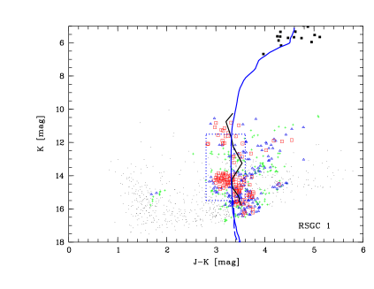
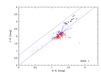
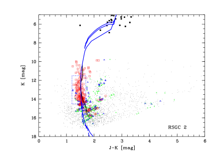
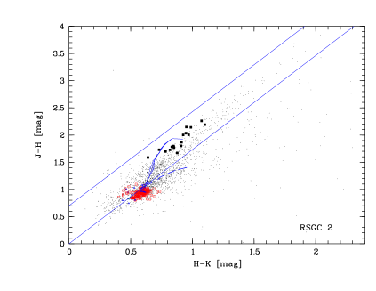
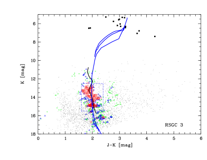
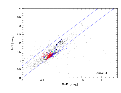
Figure 1: Colour-Magnitude (left) and Colour-Colour (right) diagrams for RSGC 1 (top), RSGC 2 (middle) and RSGC 3 (bottom). Objects brighter than $K$ = 8 mag are stars detected by 2MASS within 3′ of the cluster centre and are shown as black filled squares. The remaining stars are from our PSF photometry. The colour coding indicates the photometric cluster membership probability of the stars: $P^{i}_{cl}>70\,\%$ red squares; $60\,\%\leq P^{i}_{cl}<70\,\%$ blue triangles; $50\,\%\leq P^{i}_{cl}<60\,\%$ green plus signs; $P^{i}_{cl}<50\,\%$ black dots. In the CMDs, the black solid line indicates the average position of the most likely cluster members, the blue solid line an isochrone from Lejeune & Schaerer (2001) (using the ages listed in Table 2) and the blue dashed line an isochrone from Siess et al. (2000). The dotted boxes indicate the region of stars overplotted on the CCDs. The reddening band in the CCDs is based on the extinction laws from Indebetouw et al. (2005).

Table 2: Here we list the properties of the RSGC clusters and the parameters of the isochrones overplotted on the CMDs and CCDs. We list the radius $r$ out to which we include stars in the photometric decontamination, the adopted distance and age of the cluster, as well as the $K$-band extinction determined in the literature $A^{Lit}_{K}$ for the cluster RSGs and the extinction $A^{MS}_{K}$ determined from our isochrone fit to the cluster main sequences. $\Delta A^{MS}_{K}$ indicates the width of the main sequence, i.e. the differential reddening. In $K^{3}_{MS}$ and $K^{10}_{MS}$ we list the apparent $K$-band magnitude for which there are at least 3 (or 10) main sequence members (weighted by their membership probability) per 0.5 mag bin. The numbers in brackets indicate the absolute magnitudes of these objects de-reddened with our extinction. $N_{MS}^{>8\,M_{\odot}}$ is the number of potential massive main sequence stars (weighted by their membership probability) brighter than $M_{K}$ = -0.9 mag and $N_{RSG}$ the number of spectroscopically confirmed RSGs in the cluster from the literature. See text for details.

Name	r	d	age	$A^{Lit}_{K}$	$A^{MS}_{K}$	$\Delta$$A^{MS}_{K}$	$K^{3}_{MS}$	$K^{10}_{MS}$	$N_{MS}^{>8\,M_{\odot}}$	$N_{RSG}$
	[  ′ ]	[kpc]	[Myrs]	[mag]	[mag]	[mag]	[mag]	[mag]
RSGC 1	1.5	6	10	2.74	2.3	0.75	10.5 (-5.9)	12.5 (-3.7)	210	14
RSGC 2	1.8	6	17	1.47	1.0	0.25	10.0 (-5.0)	11.0 (-4.0)	115	26
RSGC 3	1.8	6	20	1.50	1.4	0.25	11.5 (-3.6)	13.0 (-2.1)	115	16

3 Results

Here we discuss the results obtained for all the investigated clusters. Some further details on the individual objects can be found in Appendix A.

3.1 General

Theoretically one would expect the main sequence of these massive clusters to appear as a vertical accumulation of high probability cluster members in a $K$ vs. $J$$-$$K$ colour-magnitude diagram (CMD), since most stars visible should be of high mass and thus have similar intrinsic near infrared colours. Some scatter in colour is expected due to differential reddening along the line of sight. Furthermore, these high mass main sequence stars should be situated at the bottom of the reddening band in a near infrared $H$$-$$K$ vs. $J$$-$$H$ colour-colour diagram (CCD) and not in the middle/top, which is usually occupied by giant stars.

In the left column of panels in Fig. 1 we show as examples the decontaminated $K$ vs. $J$$-$$K$ CMD of RSGC 1, 2, 3. All stars fainter than 8^th magnitude in $K$ are from our PSF photometry. All bright, potential RSGs (large black squares) are taken from 2MASS since they are saturated in the UKIDSS images. All small black dot symbols are stars in the cluster area with less than 50 % cluster membership probability $P^{i}_{cl}$. Green plus signs indicate stars with $50\,\%\leq P^{i}_{cl}<60\,\%$, blue triangles stars with $60\,\%\leq P^{i}_{cl}<70\,\%$ and red squares $P^{i}_{cl}>70\,\%$.

We determined a running weighted average of the $J$$-$$K$ colours of the most likely cluster members along the detected main sequence. This is indicated by the solid black line in the CMDs in Fig. 1. As weighting factor for each star we used the square of the membership probability $P^{i}_{cl}$. To compare the cluster data with model isochrones, we utilise the Geneva isochrones by Lejeune & Schaerer (2001) which are overplotted in each panel as a blue solid line, using the parameters specified in Table 2. We also overplot as a dashed line the isochrones for low and intermediate mass stars from Siess et al. (2000).

In the right column of panels in Fig. 1 we show the corresponding $H$$-$$K$ vs. $J$$-$$H$ CCDs for the same three clusters. Symbols and colours are identical in their meaning to the CMDs. However, we plot all stars in the field as small black dots and only high probability cluster members ($P^{i}_{cl}>50\,\%$) from the potential main sequences (as indicated by the dotted boxes in the CMDs) are shown in large coloured symbols. These boxes exclude bright, potentially saturated stars as well as faint, low signal to noise objects and obvious background giants. The indicated reddening band for each cluster indicated, is based on the reddening law by Indebetouw et al. (2005).

From all the clusters investigated, we can detect a main sequence only in the known objects RSGC 1, 2 and 3 (see Fig. 1). We also investigated the fields around RSGC 4 (Negueruela et al., 2010) and RSGC 5 (Negueruela et al., 2011) but there are no apparent overdensities of stars, in particular none that would indicate a main sequence (see Fig. D1 in the Appendix). There are several possibilities that could explain this. i) These clusters have less mass, i.e. fewer members, than the other objects and thus they do not manifest themselves as overdensities in colour magnitude space. ii) The clusters are much more extended spatially than our search area for potential main sequence stars; they are more association like in appearance than cluster like. Both points seem to contribute, since both clusters have fewer confirmed members than the brighter RSGCs and they seem to be embedded in more extended regions of massive young stars (Negueruela et al., 2010; Negueruela et al., 2011).

For the new cluster candidates F 3 and F 4 from Froebrich (2013) only features that look like a tentative MS in the CMDs are found (see Fig. D2 in the Appendix). For F 3, a clump of stars at $K$ = 13 mag and $J$$-$$K$ = 2.4 mag can be identified, while for F 4 a more MS like feature can be seen at $J$$-$$K$ = 2.6 mag. Both of these features contain a few hundred high probability members. However, when utilising the CCDs for both cluster candidates, one can identify that these features are not caused by main sequence stars. The high probability members clearly are not situated near the bottom of the reddening band, indicating they are giants. Only in the case of F 3, there are some potential main sequence stars. Thus, both candidates are most likely holes in the general extinction and not real clusters.

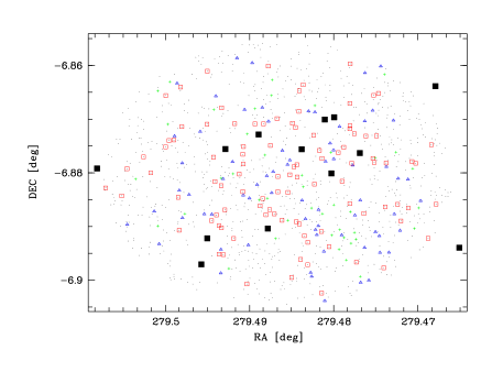
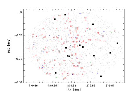
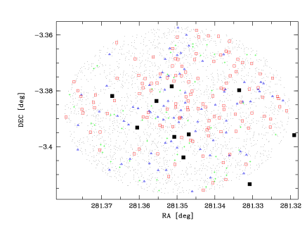
Figure 2: Positions of the stars in RSGC 1 (top), RSGC 2 (middle) and RSGC 3 (bottom). Colour coding is the same as in Fig. 1. Only stars which are suspected MS stars (objects in the blue dotted boxes in the CMDs in Fig. 1) are plotted as coloured symbols while the remaining stars in the field are represented by black dots and confirmed RSGs are shown as black filled squares.

3.2 Main Sequence Properties

Here we will concentrate on determining the principle properties of the detected main sequences for RSGC 1, 2 and 3. The isochrones overplotted to the CMDs and CCDs use age and distance estimates from the literature (see Table 2 for these parameters). We adopt a distance of 6 kpc for all clusters, which seems an appropriate average of the published values (Figer et al., 2006; Davies et al., 2008; Davies et al., 2007; Clark et al., 2009; Alexander et al., 2009). The ages are taken for each individual cluster from the same references. We only vary the extinction in the $K$-band to shift the isochrone onto the detected main sequence. Since the upper end of the MS is almost vertical in the $K$ vs. $J$$-$$K$ CMDs, the actual choise of age and distance will not influence the required extinction value.

All main sequences are ’vertical’ in the CMDs for the top 2 – 4 mag in the $K$-band. Hence, these are clearly massive MS stars and we can try to estimate the colour excess towards the cluster by shifting an isochrone until it fits the MS. This will determine the extinction towards potential cluster members, i.e. the column density of material along the line of sight that is not associated with the cluster itself, and is independent of the actual age chosen for the isochrone. Utilising an extinction law (we use Indebetouw et al. (2005)), we can convert this to a foreground extinction value. These are the values we used to overplot the isochrones in Fig. 1 and which are listed as $A_{K}^{MS}$ in Table 2. In the colour-colour diagrams in the right hand side panels of Fig. 1 one can see that the reddening direction of the background giants confirms the validity of this reddening law. In essence the reddening law in these fields is in agreement with Indebetouw et al. (2005) or Stead & Hoare (2009), but using a less steep dependence of extinction on wavelength such as in Mathis (1990) or Rieke & Lebofsky (1985) can be ruled out from the CCDs. Thus, please note that the use of an extinction law in agreement with the CCDs will change the infered $K$-band extinction by only about 0.1 mag. However, larger differences are expected when a less steep extinction law is applied. The cluster RSGC 1 has the largest extinction of 2.4 mag in the $K$-band, while the other two clusters have about half this value of reddening, i.e. $A_{K}$ $\approx$ 1.2 mag. Compared to the literature values (listed as $A_{K}^{Lit}$ in Table 2), our isochrone fit to the main sequence systematically finds smaller extinction values. This could be caused by the fact that: i) the literature extinction values are estimated using a different extinction law (such as by Davies et al. (2007) for RSGC 2); ii) the observations are taken in different filters, e.g. 2MASS $K_{S}$ vs. UKIDSS $K$; iii) the extinction values are determined from the spectral types of the red supergiants in the cluster and not by the better understood main sequence stars. Recently Davies et al. (2013) have shown that there can indeed by issues with the RSG temperature scale.

We further estimate the amount of material associated with the cluster itself. This can be done by measuring the width of the main sequence in $J$$-$$K$ and convert this to a value of differential reddening. We list these values in the $\Delta A_{K}$ column in Table 2. As for the general interstellar extinction, RSGC 1 shows the highest amount of differential reddening with about 0.75 mag in the $K$-band. This is about three times as high as for the other two clusters, but comparable to, or even smaller than for other young embedded clusters (e.g. the Orion Nebula Cluster (Scandariato et al., 2011)). There are several possible explanations for the differences: i) This cluster is younger and thus still more deeply embedded in its parental molecular cloud – however this is unlikely given the age of the cluster. ii) The differential reddening is not caused by intrinsic dust, but by the variations in extinction of the foreground material. The larger value for $A^{MS}_{K}$ for this cluster could support this.

In order to investigate the number of potential main sequence stars in each cluster we defined a colour range in $J$$-$$K$ for each cluster (as indicated in the CMDs in Fig. 1) that encloses all the potential MS stars. We select all stars within this colour range and determine the $K$-band luminosity function along the main sequence. These are shown as dotted blue lines in Fig. E1 in the Appendix. If we only count the membership probabilities $P^{i}_{cl}$ for each star, then we obtain a more realistic luminosity function which is shown as solid red line in Fig. E1. The smallest difference between the two luminosity functions is evident for RSGC 2. Thus, this is the cluster where the MS stands out most significantly from the field stars. This is in agreement with the fact that this is the only cluster where the main sequence has been detected previously (Froebrich, 2013). The typical membership probability for the MS cluster members is about 80 % for RSGC 2, while it is of the order of 60 % for the other two clusters.

We investigate the brightest MS stars in each cluster and define $K^{3}_{MS}$ as the apparent $K$-band magnitude where there are at least three stars per 0.5 mag bin along the MS. In other words we treat this as the top of the main sequence. Similarly we define $K^{10}_{MS}$ and list both values in Table 2. The most populated cluster main sequence at bright $K$-band magnitudes occurs in RSGC 2. There, $K^{10}_{MS}$ = 11 mag, while $K^{3}_{MS}$ is one magnitude brighter. RSGC 3 has by far the fewest bright cluster main sequence stars, or the MS starts only at fainter magnitudes. The absolute magnitudes for $K^{3}_{MS}$ and $K^{10}_{MS}$ are determined from our adopted distance and de-reddened with $A_{K}^{MS}$. They are listed in brackets in Table 2 and show that RSGC 1 has the brightest ($M_{K}$ = -5.9 mag) end of the MS while RSGC 3 has intrinsically the faintest end of the MS ($M_{K}$ = -3.7 mag). This is in good agreement with the ages for the clusters determined in the literature, which range from 8 – 12 Myrs for RSGC 1 (Figer et al., 2006; Davies et al., 2008) to about 20 Myrs for RSGC 3 (Alexander et al., 2009). Note that according to the isochrones used (Lejeune & Schaerer, 2001), stars with a mass above 20 M_⊙ (or O-type stars) have $M_{K}$ = -2.9 mag or brighter on the MS. Thus, in particular RSGC 1 and RSGC 2, could contain a significant number of massive MS or post-MS objects, that can easily be verified spectroscopically. Note that the total number of these cluster members is likely to be larger by about 50 %, since we have only analysed the stars within one cluster radius. There are spectroscopically confirmed cluster members in the region between one a two cluster radii; typically only about 2/3^rd of the known members are within one cluster radius.

The completeness limit determined as the peak of the $K$-band luminosity function, for all clusters is between $K$ = 15 mag and 16 mag. In all cases, this is fainter than stars of about 8 M_⊙ which have $M_{K}$ = -0.9 mag (Lejeune & Schaerer, 2001) or an apparent magnitude of $K$ = 13.0 mag at our adopted distance and without considering extinction. We thus can compare the total number of stars along the main sequence, brighter than these stars. The numbers are weighted by the membership probabilities and are listed as $N_{MS}^{>8\,M_{\odot}}$ in Table 2. We find that RSGC 1 has about twice as many of these OB-type stars than RSGC 2 and 3. Please note that we expect increased crowding in the cluster centres and thus the estimated OB-type cluster member numbers should be treated as lower limits. Since RSGC 1 is the most compact of the three clusters, its numbers should be most affected. The number of confirmed RSGs (see column $N_{RSG}$ in Table 2) in RSGC 2 is much higher than in RSGC 1, which might be due to the lower age of the latter. Hence, out of the three clusters, RSGC 1 seems to be the most massive object as estimated in Figer et al. (2006) and Davies et al. (2008). Based on the number of stars along the main sequence and the age, RSGC 2 and 3 might be less massive, partly (for RSGC 3) in agreement with the predictions from Alexander et al. (2009) and at the lower end of the mass range suggested in Clark et al. (2009).

In Fig.2 we show the spatial distribution of all stars along the MS for the three clusters. Only stars within the cluster radius are shown, since we have not determined membership probabilities outside this area. In all three cases the most likely MS stars are concentrated towards the nominal centre of the clusters. However, the distribution seems not be centrally condensed, but rather filamentary, especially for RSCG 2. If this is a real effect, or caused by crowding in the cluster centre and ’missing’ objects near the bright RSGs is unclear. The spatial density of the main sequence cluster members (each star is weighted by its membership probability) is between two and three times higher in the cluster centre compared to the outer regions as defined by the cluster radius.

4 Conclusions

We have used PSF photometry on deep NIR JHK imaging data from the UKIDSS GPS to investigate the fields of known and candidate red supergiant clusters. We confirm the detection by Froebrich (2013) of the upper main sequence of the cluster RSGC 2 and for the first time detect the main sequence for RSGC 1 and RSGC 3.

We use the age and distance estimates from the literature to overplot isochrones on the NIR colour-magnitude diagrams for all clusters in order to establish the reddening of the main sequences by utilising the reddening law from Indebetouw et al. (2005). In all cases the infered $K$-band extinction values for the main sequences are smaller than the quoted values in the literature, which are determined for the red supergiant stars. We also infer the differential reddening towards each cluster based on the width of the detected main sequence. The youngest of the clusters (RSGC 1) has the highest extinction and differential reddening in accordance with its evolutionary status. It also contains the most number of stars (about 200) with masses above 8 $M_{\odot}$.

The spatial distribution of the candidate main sequence stars in all clusters shows a concentration towards the nominal cluster centre. However, there is no indication of a centrally condensed distribution, which could either be real or caused by increased crowding and blending effects from the bright red supergiant cluster members.

We also investigated fields near the clusters RSGC 4 and RSGC 5, as well as the candidate RSG clusters F 3 and F 4 from Froebrich (2013). In all cases no main sequence could be detected. In the case of the already known clusters this could be caused by them having less members or being spatially more extended, i.e. more association like. Our results indicate that the new candidates can most likely be interpreted as holes in the background extinction.

References

- Alexander et al. (2009) Alexander M. J., Kobulnicky H. A., Clemens D. P., Jameson K., Pinnick A., Pavel M., 2009, Astronomical Journal, 137, 4824
- Bonatto & Bica (2007) Bonatto C., Bica E., 2007, Monthly Notices of the RAS, 377, 1301
- Bonatto et al. (2004) Bonatto C., Bica E., Girardi L., 2004, Astronomy and Astrophysics, 415, 571
- Clark et al. (1998) Clark J. S., Fender R. P., Waters L. B. F. M., Dougherty S. M., Koornneef J., Steele I. A., van Blokland A., 1998, Monthly Notices of the RAS, 299, L43
- Clark et al. (2009) Clark J. S., Negueruela I., Davies B., Larionov V. M., Ritchie B. W., Figer D. F., Messineo M., Crowther P. A., Arkharov A. A., 2009, Astronomy and Astrophysics, 498, 109
- Davies et al. (2007) Davies B., Figer D. F., Kudritzki R.-P., MacKenty J., Najarro F., Herrero A., 2007, Astrophysical Journal, 671, 781
- Davies et al. (2008) Davies B., Figer D. F., Law C. J., Kudritzki R.-P., Najarro F., Herrero A., MacKenty J. W., 2008, Astrophysical Journal, 676, 1016
- Davies et al. (2013) Davies B., Kudritzki R.-P., Plez B., Trager S., Lançon A., Gazak Z., Bergemann M., Evans C., Chiavassa A., 2013, Astrophysical Journal, 767, 3
- Figer et al. (2006) Figer D. F., MacKenty J. W., Robberto M., Smith K., Najarro F., Kudritzki R. P., Herrero A., 2006, Astrophysical Journal, 643, 1166
- Froebrich (2013) Froebrich D., 2013, International Journal of Astronomy and Astrophysics, 3, 161
- Froebrich et al. (2010) Froebrich D., Schmeja S., Samuel D., Lucas P. W., 2010, Monthly Notices of the RAS, 409, 1281
- Gvaramadze et al. (2012) Gvaramadze V. V., Weidner C., Kroupa P., Pflamm-Altenburg J., 2012, Monthly Notices of the RAS, 424, 3037
- Indebetouw et al. (2005) Indebetouw R., Mathis J. S., Babler B. L., Meade M. R., Watson C., Whitney B. A., Wolff M. J., Wolfire M. G., 2005, Astrophysical Journal, 619, 931
- Lawrence et al. (2007) Lawrence A., Warren S. J., Almaini O., Edge A. C., Hambly N. C., Jameson R. F., Lucas P., Casali M. E., 2007, Monthly Notices of the RAS, 379, 1599
- Lejeune & Schaerer (2001) Lejeune T., Schaerer D., 2001, Astronomy and Astrophysics, 366, 538
- Lucas et al. (2008) Lucas P. W., Hoare M. G., Longmore A., Schröder A. C., Davis C. J., Adamson A., Bandyopadhyay R. M., de Grijs R., 2008, Monthly Notices of the RAS, 391, 136
- Marco & Negueruela (2013) Marco A., Negueruela I., 2013, Astronomy and Astrophysics, 552, A92
- Mathis (1990) Mathis J. S., 1990, Annual Review of Astron and Astrophysics, 28, 37
- Negueruela et al. (2011) Negueruela I., González-Fernández C., Marco A., Clark J. S., 2011, Astronomy and Astrophysics, 528, A59
- Negueruela et al. (2010) Negueruela I., González-Fernández C., Marco A., Clark J. S., Martínez-Núñez S., 2010, Astronomy and Astrophysics, 513, A74
- Oey et al. (2013) Oey M. S., Lamb J. B., Kushner C. T., Pellegrini E. W., Graus A. S., 2013, Astrophysical Journal, 768, 66
- Ortolani et al. (2002) Ortolani S., Bica E., Barbuy B., Momany Y., 2002, Astronomy and Astrophysics, 390, 931
- Piatti et al. (1998) Piatti A. E., Bica E., Claria J. J., 1998, Astronomy and Astrophysics, Supplement, 127, 423
- Rahman et al. (2013) Rahman M., Matzner C. D., Moon D.-S., 2013, Astrophysical Journal, 766, 135
- Rieke & Lebofsky (1985) Rieke G. H., Lebofsky M. J., 1985, Astrophysical Journal, 288, 618
- Scandariato et al. (2011) Scandariato G., Robberto M., Pagano I., Hillenbrand L. A., 2011, Astronomy and Astrophysics, 533, A38
- Siess et al. (2000) Siess L., Dufour E., Forestini M., 2000, Astronomy and Astrophysics, 358, 593
- Skrutskie et al. (2006) Skrutskie M. F., Cutri R. M., Stiening R., Weinberg M. D., Schneider S., Carpenter J. M., Beichman C., Capps R., 2006, Astronomical Journal, 131, 1163
- Stead & Hoare (2009) Stead J. J., Hoare M. G., 2009, Monthly Notices of the RAS, 400, 731
- Stephenson (1990) Stephenson C. B., 1990, Astronomical Journal, 99, 1867
- Stetson (1987) Stetson P. B., 1987, Publications of the ASP, 99, 191
- Westerlund (1961) Westerlund B., 1961, Publications of the ASP, 73, 51