Cavity polariton in a quasi-lattice of qubits and its selective radiation

Abstract

In a circuit quantum eletrodynamic system, a chain of $N$ qubits inhomogeneously coupled to a cavity field forms a mesoscopic quasi-lattice, which is characterized by its degree of deformation from a normal lattice. This deformation is a function of the relative spacing, that is the ratio of the qubit spacing to the cavity wavelength. A polariton mode arise in the quasi-lattice as the dressed mode of the lattice excitation by the cavity photon. We show that the transition probability of the polariton mode is either enhanced or decreased compared to that of a single qubit by the deformation, giving a selective spontaneous radiation spectrum. Further, unlike a microscopic lattice with large-$N$ limit and nearly zero relative spacing, the polariton in the quasi-lattice has uneven decay rate over the relative spacing. We show that this unevenness coincides with the cooperative emission effect expected from the superradiance model, where alternative excitations in the qubits of the lattice result in maximum decay.

I Introduction

I.1 Quasi-lattices of qubits

Superconducting qubits are a class of two-level systems based on the superconducting Josephson junctions clarke08 . When interacting with a microwave field stalled in a stripline resonator, they act like artificial atoms in optical cavities with coherent exchange of photon energy modeled on the Jaynes-Cummings Hamiltonian wallraff04 ; majer07 . This combination gives rise to circuit quantum electrodynamics (QED) blais04 , an emulation of cavity QED. Circuit QED systems with superconducting qubits can therefore emulates, in many aspects, quantum optical effects similar to those originally discovered on real atoms or atomic media jqyou11 and can be regarded as a type of quantum simulators buluta09 .

So far, studies of circuit QED only concerns with circuits of a few superconducting qubits and each qubit is considered acting separately with the stripline resonator. To understand their collective behavior, a many-qubit theory is wanted. However, traditional many-atom theories such as the Frenkel model for excitons cannot not be applied because circuit QED systems contain only a finite number of artificial atoms, i.e., large-$N$ limit is not taken. Neither do models for finite $N$, such as the Tavis-Cummings (TC) model tavis68 apply because the mesoscopic sizes of the qubits and of the spacings between the qubits in a circuit make their dipole-field interaction to the stripline resonator inhomogeneous. To remedy the inapplicability, we have proposed a projection-deformation model that generalizes the TC-model to work on inhomogeneous coupling scenarios ian12 ; ian13 .

The basic idea is that while real atoms form a lattice, the superconducting qubits form a quasi-lattice, whose “quasi-ness” is measured by the degree of deformation it departs from a normal lattice. This deformation is related to a deformed SU(2) algebra sun89 obeyed by the collective spin operators of the quasi-lattice and is quantified by a c-number deformation factor. This factor is parametrized by the ratio of the uniform lattice spacing $L_{\mathrm{q}}$ to the wavelength $\lambda_{\mathrm{p}}$ of the interacting photon. We call this ratio the relative spacing $\ell$ of the qubits. The analytical excitation spectrum of the quasi-lattice can then be computed by diagonalizing the deformation-dependent interaction Hamiltonian.

I.2 Polariton and the radiation problem

The excited states of the quasi-lattice ought to spontaneously radiate microwave photons into the circuit waveguide. But in a circuit QED system, the excitation mode of the quasi-lattice is coherently coupled to a stripline resonator mode, where the mixed mode of the two forms a cavity polariton. Therefore, unlike the conventional radiation problems treated in atomic physics, such as the Dicke radiation dicke54 ; ernst68 , the radiation in the mesoscopic circuit cavity is associated with the dynamics of the polariton, i.e. a dressed quasi-lattice excitation mode, instead of a bare lattice excitation mode.

It is known that, in a dielectric, the polariton mode is generated by the recombination of the collective atomic excitations with the radiated photons knoester89 . The polariton mode we treat here, on the other hand, is generated by the dressing through the cavity photon. The definition is similar to that given in semiconductor cavity QED systems keeling07 ; savona94 . The radiated photon modes are designated in a separate Hilbert space from that of the cavity photon mode. Therefore, even though the radiation processes are both polariton-mediated, the case for a quasi-lattice of qubits is vastly different from the case of a dielectric.

Besides, the energies and the eigenstates of the quasi-lattice excitation modes are modified by the deformation described above. The composition of the Fock number states of the polariton depends thus not only on the eigenenergy of the qubits, but also on the deformation of the quasi-lattice. It was shown that the structure of the underlying medium has a large influence on the pattern and form of the radiation. For example, the spontaneous emission is found directionally dependent on the incident photon scully06 in an extended medium; uneven decay rates is found in a spherical symmetric medium by including virtual photon processes svidz10 ; and nonlocal effect arises for single-photon cooperative emission svidz12 . The purpose of this paper is to investigate how the structural change introduced by the deformation of the quasi-lattice affects the radiation spectrum and the polariton decay.

We find that the cavity polariton has an acutely selective distribution of its radiated microwave photon based on the deformation. This is shown by the varying amplitude of the interaction coefficient between the polariton and the continuum of photon modes in the momentum space. This amplitude depends on the relative spacing and has a quasi-periodicity that matches this relative spacing with the wavelength of the cavity photon, demonstrating the selectiveness of the quasi-lattice about its radiation. Specifically, at the exact periodic positions where the radiated photon resonates with the cavity, the magnitude of the interaction will obtain its maximum value.

Moreover, we find that the polariton decay is also deformation-dependent on the relative spacing. In fact, as predicted by Dicke, the decay rate of an $N$-atom lattice would increase to $N^{2}$ when the spin moment of the lattice is at the maximum cooperation number of $N/2$, giving rise to superradiance rehler71 ; macgill76 ; ressayre77 and superfluorescence bonifacio75 ; glauber78 ; polder79 . For the quasi-lattice of qubits, it is found that the maximum decay rate is obtained when the relative spacing is set to one half, where only every other qubit couples to the cavity photon. This alternate pattern of coupling excites half of the qubits while leaving the other half unaffected, giving an effective spin moment of $N/2$ to the quasi-lattice and having the decay rate match with the Dicke model of cooperated radiation.

The article is organized as follows. The formation of cavity polariton in a quasi-lattice is given in Sec. II, where the transition matrices for the quasi-lattice as deformed SU(2) spin is derived in the polariton basis. By writing the qubit operators terms of these matrices using a discrete Fourier transform, we derive the expression of the quasi-periodic interaction coefficient for radiation in Sec. IIIA. As an example, the simplest non-trivial case with $N=4$ is plotted especially to illustrate the uneven distribution of radiation of the mesoscopic system. With the derived interaction coefficient, the equation of motion for the low-energy polariton states are derived in Sec. IIIB. The decay rate of the polariton is subsequently computed under the Markov and the Wigner-Weisskopf approximations in Sec. IV. The conclusion and relevant discussions are given in Sec. V.

II Polaritons

II.1 System state space

Consider the circuit QED system illustrated in Fig. 1 with $N$ superconducting qubits (indicated by gray squares), where two neighboring ones are spaced at a uniform distance $L_{\mathrm{q}}$. Each qubit can be modeled as a two-level system $\sigma_{j,z}$ in the diagonalized basis of the Josephson and charge energies of the junctions that it contains. Depending on the type of the qubit, the diagonalized eigenenergy is tunable through magnetic flux, gate charge, phase, etc. and we consider the $N$ qubits are tuned uniform with level spacing $\omega_{\mathrm{q}}$ in our study here.

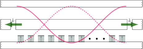
Figure 1: (Color online) Schematic of a quasi-lattice chain of qubits coupled to a cavity field. The arrow $k$ indicates the direction of photons radiated by the polaritons formed from the excitation of the quasi-lattice and the cavity field.

The middle rectangular strip indicates the coplanar waveguide or stripline resonator, which is equivalent to a cavity and contains multiple modes of a standing microwave field. However, when the qubits are all tuned resonant with the fundamental mode, the cavity field can be effectively regarded as a single-mode field fink09 ; macha13 . We describe this fundamental mode (the red curve in the figure) by the annihilation operator $\bar{a}$ and denote its frequency and wavelength by $\omega_{\mathrm{C}}$ and $\lambda_{\mathrm{C}}$, respectively. Note that even though the dimensions of a qubit are negligible compared to the wavelength $\lambda_{\mathrm{C}}$, the spacings between the qubits are non-negligible and the coupling of each qubit to the cavity field depends on the relative spacing $\ell=2L_{\mathrm{q}}/\lambda_{\mathrm{C}}$ described above through a sinusoidal factor $\cos(j\pi\ell)$. The variable $j$ consequently can be regarded as a relative coordinate for the qubits along the one-dimensional chain of qubits. This chain of qubits can be regarded as a quasi-lattice, which resembles an atomic lattice but has an inhomogeneous coupling due to its mesoscopic nature.

This quasi-lattice of qubits is also environmentally coupled to a reservoir, represented by a continuum of quantum oscillators $\{a_{k}\}$ with frequency spectrum $\omega_{k}$, which gives rise to spontaneous radiation in and out of the waveguide. These radiated photons carry momentum $k$ and are illustrated as the green arrows in Fig. 1. Their propagations in the waveguide are indicated by the wave functions $e^{ikr_{j}}$, where $r_{j}$ is the coordinate of the associated qubit. Note that, unlike the treatments for radiation in atomic media where confinements in pencil-shape geometries are usually assumed ressayre77 ; bonifacio75 , the waveguide in superconducting circuits are strictly one-dimensional and thus $k$ is regarded as a wave number, not a wave vector.

The total system Hamiltonian is therefore divided into three parts and can be written as follows (assuming $\hbar=c=1$)

$$H = H_{\mathrm{sys}}+V_{\mathrm{cav}}+V_{\mathrm{rad}},$$ (1)

$$H_{\mathrm{sys}} = \omega_{\mathrm{q}}\sum_{j=0}^{N-1}\sigma_{j,z}+\omega_{\mathrm{C}}\bar{a}^{\dagger}\bar{a},$$ (2)

$$V_{\mathrm{cav}} = \eta\sum_{j=0}^{N-1}\cos(j\pi\ell)\left[\sigma_{j,+}\bar{a}+\sigma_{j,-}\bar{a}^{\dagger}\right],$$ (3)

$$V_{\mathrm{rad}} = \sum_{j=0}^{N-1}\sum_{k}g_{k}\left(a_{k}\sigma_{j,+}e^{ikr_{j}}+a_{k}^{\dagger}\sigma_{j,-}e^{-ikr_{j}}\right).$$ (4)

Note that the forms taken by Eqs. (2)-(3) assumes a strong coupling operation regime for the qubits, where each qubit has a maximal coupling strengh $\eta$ much greater than the linewidth of the circuit cavity, to ensure coherent exchange of photons with the circuit cavity while the non-rotating wave terms for the virtual photons can be ignored majer07 . Further, based on the current experiment setups macha13 , the magnitude of $\eta$ is much smaller than $\omega_{\mathrm{q}}$ such that the quasi-lattice system on the other hand does not enter into the ultra-strong coupling (USC) regime. When $\eta$ is comparable to $\omega_{\mathrm{q}}$, USC operation will dominate and squeezing terms of $a$ and $a^{\dagger}$ have to be taken into considerations deliberato14 . These terms entail complex implications to Dicke phase transitions on circuit QED systems nataf10 ; viehmann11 .

The relevant Hilbert space is tripartite:

$$\mathcal{H}=\mathcal{Q}^{\otimes N}\times\mathcal{U}\times\prod^{\otimes k}\mathcal{V}_{k},$$ (5)

where each $\mathcal{Q}=\mathrm{span}\{\left|\uparrow\right\rangle,\left|\downarrow\right\rangle\}$ is the internal energy eigenspace for a qubit, $\mathcal{U}=\mathrm{span}\{\left|0\right\rangle,\left|1\right\rangle,\left|2\right\rangle,\dots\}$ is the Fock eigenspace for the cavity photon, and each $\mathcal{V}_{k}=\mathrm{span}\{\left|0\right\rangle_{k},\left|1\right\rangle_{k},\left|2\right\rangle_{k},\dots\}$ is the Fock eigenspace for spontaneous emitted photon of wave number $k$. A specific system state vector, for example, in this tripartite Hilbert space can be written as

$$\left|\downarrow\uparrow\downarrow\downarrow\cdots\uparrow\right\rangle\otimes\left|n\right\rangle\otimes\left|\{k_{j}\}\right\rangle,$$ (6)

where the first subvector denotes the configuration of the quasi-lattice of qubits, the second that of cavity photon number, and the third that of the photon momentum radiated by each qubit in the quasi-lattice.

Following the idea of either Dicke or Tavis-Cummings, the quasi-lattice can be equally expressed in the angular momentum space $\left|r,m\right\rangle$ where $r=N/2=\frac{1}{2}(n_{\uparrow}+n_{\downarrow})$ is the total quantized spin and $m$ the magnetic moment. $m$ is also the difference between the number of spin-up qubits and the number of spin-down qubits in the quasi-lattice, i.e. $m=\frac{1}{2}(n_{\uparrow}-n_{\downarrow})\in\{-r,-r+1,\dots,r\}$. Hence, a quasi-lattice state expressed in $\left|r,m\right\rangle$ space has the following correspondence to the qubit spin states

$$\left|r,m\right\rangle=\sqrt{\frac{(r+m)!(r-m)!}{2r!}}\sum_{p}\Pi_{p}\left|\underbrace{\uparrow\uparrow\cdots\uparrow}_{r+m}\underbrace{\downarrow\downarrow\cdots\downarrow}_{r-m}\right\rangle,$$ (7)

where $\Pi_{p}$ is a permutation operation on the ordered spin state $\left|\uparrow\uparrow\cdots\uparrow\downarrow\downarrow\cdots\downarrow\right\rangle$ and the summation is over all permutations of the same $m$. In other words, the number of permutations is the degeneracy of the state $\left|r,m\right\rangle$, which is just the reciprocal of the constant in front of the summation in Eq. (7).

Corresponding to this angular momentum space representation of the state of the quasi-lattice, we introduce a set of total angular momentum operators

$$S_{z} = \sum_{j=0}^{N-1}\sigma_{j,z},$$ (8)

$$S_{+} = \sum_{j=0}^{N-1}\cos(j\pi\ell)\sigma_{j,+},$$ (9)

and $S_{-}=(S_{+})^{\dagger}$ to replace the Pauli operators for the individual qubits. These operators obey the structure of a deformed SU(2) algebra sun03 , i.e. we have the commutator become

$$[S_{+},S_{-}]=2\Sigma_{z}$$ (10)

where $\Sigma_{z}$ is an operator function of $S_{z}$ and $\sigma_{j,z}$ with coefficients depending on $N$ and the relative spacing $\ell$ ian12 . When $N\to\infty$ and $\ell\to 0$, the coefficients in front of $\sigma_{j,z}$ vanish and $\Sigma_{z}=S_{z}$, for which the normal SU(2) algebra is reinstalled. With the introduction of these operators, the expressions for Hamiltonians (2)-(3) can be simplified to

$$H_{\mathrm{sys}} = \omega_{\mathrm{q}}S_{z}+\omega_{\mathrm{C}}\bar{a}^{\dagger}\bar{a}$$ (11)

$$V_{\mathrm{cav}} = \eta(S_{+}\bar{a}+S_{-}\bar{a}^{\dagger})$$ (12)

II.2 Diagonalizing for polariton

The polariton state is the eigenstate that diagonlizes $H_{\mathrm{sys}}+V_{\mathrm{cav}}$ by transforming the first two product spaces in Eq. (5). It arises as the dressed state the quasi-lattice excitation by the cavity field.

Since the coupling of the quasi-lattice to the cavity is inhomogeneous, the polariton state contains implicitly a dependence on the relative spacing $\ell$. Following the projection-deformation (PD) method we have introduced ian12 ; ian13 , it can be written as the eigenstate

$$\left|u,r\right\rangle=\sum_{n}c_{n}^{(u)}\left|r,u-n;n\right\rangle,$$ (13)

where $u$ denotes the total excitation number. This number $u$ is shared between $n$ for the photon energy part and $m=u-n$ for the quasi-lattice excitation part. It can take either integer or half-integer values since $m$ can be half-integer for odd $N$ of qubits. The implicit dependence on $\ell$ is reflected in the expansion coefficients

$$c_{n}^{(u)}=\mathscr{P}_{n}^{(u)}\sum_{q=0}^{n/2}\mathfrak{f}^{q-\frac{n}{2}}\mathscr{C}_{q}^{(u)},$$ (14)

through the deformation factor

$$\mathfrak{f}=\frac{1}{2}+\frac{1}{4N}\left(1+\frac{\sin(2N-1)\pi\ell}{\sin\pi\ell}\right).$$ (15)

The expression for coefficients in Eq. (14) is found by solving a recursive relation. Recursively expanding the relation, each iteration gives a term that has the same factor

$$\mathscr{P}_{n}^{(u)}=\frac{\prod_{j=0}^{n-1}\left[\varepsilon-j\Delta\omega\right]}{\sqrt{n!(r+u)^{\underline{n}}(r-u+1)^{\bar{n}}}},$$ (16)

where $\varepsilon$ is eigenvalue for the interaction $V_{\mathrm{cav}}$ in Eq. (3) and $\Delta\omega=\omega_{\mathrm{C}}-\omega_{\mathrm{q}}$ is the qubit-cavity detuning. We have used the Pochhammer symbols $x^{\underline{n}}=x(x-1)\cdots(x-n+1)$ and $x^{\bar{n}}=x(x+1)\cdots(x+n-1)$ to simplify the notation. The factor $\mathscr{C}_{q}^{(u)}$ with a fixed $q$ can be regarded as the contribution to a $u$-number excitation mode with $q$ parts of excitation from in the quasi-lattice alone. Written explicitly, it reads

$$\mathscr{C}_{q}^{(u)}=\underset{\langle j_{1}\dots j_{k}\dots j_{n/2}\rangle}{\sum\cdots\sum}\prod_{k=1}^{q}(-\eta^{2})(j_{k}+1)\times\\ \frac{r+u-j_{k}}{v-j_{k}\Delta\omega}\cdot\frac{r-u+j_{k}+1}{v-(j_{k}+1)\Delta\omega},$$ (17)

where ,under the multi-dimensional summation, $\langle j_{1}\dots j_{k}\dots j_{n/2}\rangle$ represents the descending index set $\{\forall k<l:0\leq j_{l}\leq j_{k}-2\}$. For example, for $\frac{n}{2}=2$, the summation is two dimensional, with the first index $j_{1}\in\{0,1,2\}$ and the second index $j_{2}\in\{0\}$. Appendices B and C of Ref. ian12 gives the detailed derivation.

II.3 Excitation operators in polariton basis

The vector $\left|r,m;n\right\rangle$ represents the state of the quasi-lattice and cavity system by denoting the lattice excitation and the photon state, separately. Whereas the vector $\left|u,r\right\rangle$ represents the same combination by denoting the polariton state. Consequently, the part of the total Hamiltonian not relating to spontaneous radiation, i.e. Eqs. (11)-(12), can be written in the polariton basis

$$H_{\mathrm{sys}}+V{}_{\mathrm{cav}}=\sum_{u}\Omega_{u}\left|u,r\right\rangle\left\langle u,r\right|$$ (18)

where the eigenfrequency $\Omega_{u}$ is determined a posteriori by a recursive relation ian13 . The ladder operators $S_{+}$ and $S_{-}$ in $V_{\mathrm{cav}}$, originally indicating the collective excitation from individual qubits, should now be written as the off-diagonal elements of the transition matrix in the transformed basis as well.

To find the expression of the matrix elements, we expand the bra’s and ket’s of the polariton state vector into the two-partite form in Eq. (13). We can observe that, even though there is exchange of energy between the quasi-lattice and the cavity field, the total number $u$ of excitations is preserved over the exchange process when we disregard the energy gain and loss due to spontaneous radiation, as reflected in the interaction of Eq. (4). As a result, the diagonal elements of the transition matrices for operators $S_{+}$ and $S_{-}$ are zero in the polariton basis, as we have verified in App. A.

For the non-diagonal elements, we first observe that the non-uniformity of the quasi-lattice has the effect of reducing transition amplitudes as photons are more difficult to be either absorbed or emitted with $\mathfrak{f}\leq 1$:

$$S_{+}\left|r,u-n;n\right\rangle\\ =\sqrt{\mathfrak{f}(r-u+n)(r+u-n+1)}\left|r,u-n+1;n\right\rangle,$$ (19)

$$S_{-}\left|r,u-n;n\right\rangle\\ =\sqrt{\mathfrak{f}(r+u-n)(r-u+n+1)}\left|r,u-n-1;n\right\rangle.$$ (20)

Applying the two operation rules above, the matrix elements in the polariton basis vanish except for the first off-diagonal line because of the conservation of energy in the total excitation number $u$. This gives the raising operator as a lower off-diagonal matrix

$$[S_{+}]_{u,u-1}=\sum_{n}c_{n}^{(u)}c_{n}^{(u-1)}\sqrt{\mathfrak{f}(r+u-n)(r-u+n+1)},$$ (21)

and the lowering operator as an upper off-diagonal matrix

$$[S_{-}]_{u,u+1}=\sum_{n}c_{n}^{(u)}c_{n}^{(u+1)}\sqrt{\mathfrak{f}(r-u+n)(r+u-n+1)}.$$ (22)

Since each polariton consists of a series of combinations of photons and quasi-lattice excitations that sum up to the same total excitation number, the $(u,u-1)$-th non-zero element of $S_{+}$ in the polariton basis can be expanded as a $u+1$ by $u$ block submatrix in the photon basis of $n$. This submatrix resides under the $(u,u)$-th block matrix along the diagonal, making the transition matrix $S_{+}$ lower block off-diagonal. Corresponding, $S_{-}$ in the photon basis is upper block off-diagonal, where the $(u,u+1)$-th element expands to a $u+1$ by $u+2$ submatrix, as shown in Fig. 2.

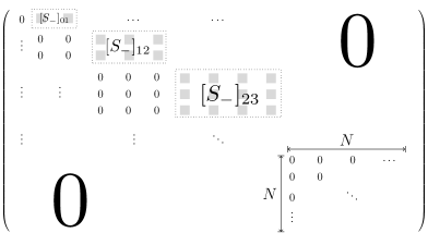
Figure 2: Matrix representation of the ladder operator $S_{-}$ in the photon basis, where the non-zero elements are clustered in blocks off the block-diagonal line.

III Equations of motion

III.1 Discrete Fourier transform and coupling coefficients

Equipped with Eqs. (21)-(22), we are ready to deal with the Hamiltonian (4) responsible for radiation. First, we need to consider the qubit operators $\sigma_{j,+}$ and $\sigma_{j,-}$ in the polariton space. This can be done by regarding the operator $S_{+}$ defined in Eq. (9) as a discrete cosine transform of $\{\sigma_{j,+}\}$. Each $\sigma_{j,+}$ can then be written as the inverse transform

$$\sigma_{j,+}=\frac{1}{N}\sum_{Nl=0}^{N-1}\cos(j\pi l)S_{l,+},$$ (23)

where we have used $Nl\in\{0,\cdots,N-1\}$ to denote the index $l\in\{0,\frac{1}{N},\dots,\frac{N-1}{N}\}$. $j$ and $l$ hence become a pair of conjugate variables for the discrete Fourier transforms such that (9) and (23) satisfy the orthonormality and unitarity conditions imposed by Parseval’s theorem.

Interpreted physically, the forward transform regards that the individual qubit excitations over all $j$ positions constitute the collective excitation, where those with $j$ at the antinodes of the cavity field contribute most to the amplitude of the collective excitation. Whereas, the inverse transform implies that the collective excitations over a set of particular $l$ constitute an individual excitation at $j$, where the more $l$ matches with $j$, the more it will contribute to the amplitude of the individual excitation.

We should emphasize that even though $l$ designates length, its meaning is distinct from $\ell$. While $\ell=2L_{\mathrm{q}}/\lambda_{\mathrm{p}}$ is a fixed value determined by the physical circuit layout, $l$ is only an indexing or transform variable that takes value from a discrete set of numbers.

Substituting the inverse transform of Eq. (23) into Eq. (4), we have the Hamiltonian in the polariton basis

$$H=\sum_{u}\Omega_{u}\left|u,r\right\rangle\left\langle u,r\right|+\sum_{k}\omega_{k}a_{k}^{\dagger}a_{k}+\\ \sum_{j,Nl=0}^{N-1}\sum_{k}\frac{g_{k}}{N}\left[a_{k}S_{l,+}\cos(j\pi l)e^{ikr_{j}}+\mathrm{h.c.}\right],$$ (24)

for which the system now essentially consists of two parts: the polaritons and the radiated photons from the polaritons. Since the collective excitation operator $S_{l,+}$ has no dependence on the relative coordinate $j$, the functions involving $j$ in the second line of the equation can be summed. Writing the coordinates $r_{j}=jL_{\mathrm{q}}=j\ell\pi/k_{0}$ where $k_{0}=2\pi/\lambda_{\mathrm{C}}$ is the momentum of the cavity photon, we find the radiation part of the Hamiltonian become

$$V_{\mathrm{rad}}=\sum_{Nl=0}^{N-1}\sum_{k}\frac{g_{k}}{N}\left[\chi_{l}(k)a_{k}S_{l,+}+\mathrm{h.c.}\right]$$ (25)

where the coefficient

$$\chi_{l}(k)=\biggl{[}1+e^{i\ell\pi(N+1)k/k_{0}}\cos l(N-1)\pi\\ -e^{i\ell N\pi k/k_{0}}\cos Nl\pi-e^{i\ell\pi k/k_{0}}\cos l\pi\biggr{]}\Bigl{/}\\ \biggl{[}1+e^{2i\ell\pi k/k_{0}}-2e^{i\ell\pi k/k_{0}}\cos l\pi\biggr{]}$$ (26)

is a function of the momentum $k$ of the radiation photon.

Comparing the interaction term of Eq. (25) with that of Eq. (4), we observe the original interaction between the individual qubits and the radiation is quantified by the dipole-field coupling amplitude $g_{k}$ only, which depends on the dipole moment of the qubits and the volume of the cavity. The coefficient $\chi_{l}(k)$ shows that an extra gain factor is introduced because the photons here are radiated from the polaritons instead of the individual qubits. Since the polaritons arises from the resonance between the quasi-lattice and the cavity, this factor $\chi_{l}(k)$ is determined by the geometric structure of the underlying quasi-lattice: the total number of qubits $N$ and the relative spacing $\ell$.

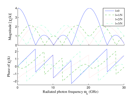
Figure 3: (Color online) (a) The magnitude and (b) the phase of the periodic coupling coefficient $\chi_{l}(k)$, for photons radiated by polaritons in the circuit QED system over a frequency range $0<\omega_{k}=ck<30$GHz. A quasi-lattice of $N=4$ qubits with relative spacing $\ell=2/3$ is assumed, for which $l$ can take four values $0$, $1/4$, $1/2$, and $3/4$.

How $N$ and $\ell$ determines the radiation character of the mesoscopic system can be illustrated from the simplest non-trivial example with an $N=4$ quasi-lattice, which is experimentally realizable in circuit QED fink09 . We take $\ell$ to be $2/3$ for a typical inhomogeneous coupling. Since $\chi_{l}$ is a complex number, its magnitude and phase are plotted separately against the radiated photon frequency in Fig. 3. In the Figure, we have assumed $k_{0}$ adopt the value based on the first harmonic given in the multi-qubit circuit by Fink et al fink09 , where $\omega_{\mathrm{C}}=ck_{0}=6.729$GHz.

We observe that the periodicity of the many exponentials in Eq. (26) makes $\chi_{l}(k)$ quasi-periodic. The quasi-period is

$$K=\frac{2k_{0}}{\ell}=\frac{\lambda_{\mathrm{C}}}{L_{\mathrm{q}}}k_{0}.$$ (27)

For the $\ell=2/3$ case plotted in the figure, the period in terms of frequency is $\omega_{K}=20.2$GHz. This quasi-periodicity matches the zeros of $|\chi_{l}|$ with the discontinuities of the phase of $\chi_{l}$ and the local maxima of $|\chi_{l}|$ with the zero phase of $\chi_{l}$. In fact, since $\chi_{l}(k)$ is an entire function of the real variable $k$, the real and the imaginary parts of $\chi_{l}(k)$ obey the Kramers-Kronig relations if we extend $k$ to the complex plane. This implies an anomalous absorption and dispersion relation of the radiation spectrum of the polariton due to the inhomogeneous coupling stephen64 .

The radiation process is therefore either enhanced or surpressed, depending on whether how well the radiation photon of frequency $\omega_{k}$ matches with the resonance between the cavity of frequency $\omega_{\mathrm{C}}$ and the quasi-lattice of relative spacing $\ell$. The fact that certain radiation range can be enhanced is because the photons emitted from these ranges are reabsorbed by the quasi-lattice before reemitting into the waveguide. From Eqs. (26)-(27), the number of extrema in $\chi_{l}$, indicating the exact matching and the exact mismatching, is determined by the number of qubits $N$ while the distance in $k$ between two such extrema is determined by the relative spacing $\ell$.

In other words, we expect the polariton radiation on a quasi-lattice of superconducting qubits provides a selective spectrum of radiation according not only to the eigenenergy of the qubits, but also to their geometric layout in the circuit. The quasi-periodic character is unique to the mesoscopic nature of the circuit QED system. For in an atomic lattice, the equivalent inter-atom spacing $L_{\mathrm{q}}$ approaches zero. The corresponding quasi-period $K$ defined by Eq. (27) will approach infinity and the periodicity vanishes.

III.2 Equations of motion

To study how exactly the varying interaction coefficient affects the radiation spectrum, we derive the equation of motion of the polariton here and compute its decay rate in the following section.

Introducing the eigenfrequency $\omega_{k}=ck$ for the radiation photon, the Hamiltonian in the interaction picture between the polariton and the radiation photon reads (see App. B for discussion)

$$H^{\prime}_{\mathrm{int}}(t)=\sum_{Nl=0}^{N-1}\sum_{k}\frac{g_{k}}{N}\left[\chi_{l}(k)a_{k}S_{l,+}e^{-i(\omega_{\mathrm{q}}-\omega_{k})t}+\mathrm{h.c.}\right].$$ (28)

To study the low-energy dynamics of multi-atom systems with weak coupling, it is customary to look at the Schroedinger equations of the lowest excited product states: states with either one excited atom across the lattice and zero photon or no excited atom and one photon scully06 ; svidz10 ; svidz12 . In the polariton basis, these two states translate into the $\mathbf{0}$-excitation state and the $\mathbf{1}$-excitation state of the dressed quasi-lattice

$$\left|\psi(t)\right\rangle=\alpha(t)\left|\mathbf{1},r\right\rangle\otimes\left|0\right\rangle+\sum_{k}\beta_{k}(t)\left|\mathbf{0},r\right\rangle\otimes\left|1_{k}\right\rangle,$$ (29)

which couple, respectively, to the zero and the one radiated photon state. The radiated photons are indexed by their momentum $k$.

Applying Schrödinger equation with the Hamiltonian (28) to this state, we find a pair of coupled equations of motion for the two coefficients of the state vector

$$\frac{\mathrm{d}\alpha}{\mathrm{d}t} = -i\sum_{Nl=0}^{N-1}\sum_{k}\frac{g_{k}}{N}\beta_{k}\chi_{l}(k)[S_{l,+}]e^{-i(\omega_{\mathrm{q}}-\omega_{k})t}$$ (30)

$$\frac{\mathrm{d}\beta_{k}}{\mathrm{d}t} = -i\sum_{Nl=0}^{N-1}\frac{g_{k}}{N}\alpha\chi_{l}^{\ast}(k)[S_{l,-}]e^{i(\omega_{\mathrm{q}}-\omega_{k})t}$$ (31)

where $[S_{+}]$ and $[S_{-}]$ are the matrix elements given by Eq. (21)-(22) for the transitions between $\mathbf{0}$-excitation state and $\mathbf{1}$-excitation state.

We note here that the coupled equations of motion are not dissimilar to those originally given for the radiation of atomic lattices. The fact that it is the polaritons undergoing the radiation is reflected by two changes to the original equations: (i) the amplitude of radiation is controlled by the extra factor $\chi_{l}(k)$ and (ii) the radiated photon is not contributed by a single excitation, but by a group of them with non-zero transition probabilities distributed in $[S_{l,\pm}]$. The weight of each contribution is determined by the deformation factor $\mathfrak{f}$ and thus by the relative spacing $\ell$ of the quasi-lattice.

To solve the coupled equations of polariton dynamics, consider that the dipole-field exchange of excitation of each qubit is a much slower process than the photon oscillation in the cavity. That means mathematically the variation of the function $\alpha(t)$ is adiabatic compared to the propagating functions $e^{i\omega_{k}t}$ and $e^{i\omega_{\mathrm{q}}t}$ of the photons. In other words, the change of $\alpha(t)$ can be computed from the average of the temporal exponentials. We hence combine Eqs. (30)-(31) and apply Markov approximation to arrive at the equation

$$\dot{\alpha}=-\sum_{k}g_{k}^{2}|\mathfrak{s}(k)|^{2}\alpha(t)\int_{0}^{t}\mathrm{d}\tau\,e^{-i(\omega_{\mathrm{q}}-\omega_{k})(t-\tau)},$$ (32)

where we have used the notation

$$\mathfrak{s}(k)=\frac{1}{N}\sum_{Nl=0}^{N-1}\chi_{l}(k)[S_{l,+}].$$ (33)

The application of Markov approximation also accords with Wigner-Weisskopf’s original treatment of atomic decay, by assuming the decaying function be exponential. That is, the exponetial function $\alpha(\tau)\approx e^{-\gamma\tau/2}$ would be a much slower process than the oscillating function $e^{-i\omega\tau}$. We follow this line of thought and derive the decay of polariton in the next section.

IV Wigner-Weisskopf approximation and decay rate

IV.1 Wigner-Weisskopf approximation

The approximation of Wigner-Weisskopf assumes a continuous radiation spectrum, so the summation over momentum $k$ can be extended to an integral and Eq. (32) reads

$$\frac{\mathrm{d}}{\mathrm{d}t}\alpha(t)=-\frac{\lambda_{\mathrm{C}}}{2\pi}\int\mathrm{d}k\,g_{k}^{2}|\mathfrak{s}(k)|^{2}\alpha(t)\frac{1-e^{-i(\omega_{\mathrm{q}}-\omega_{k})t}}{i(\omega_{\mathrm{q}}-\omega_{k})}.$$ (34)

At steady state ($t\to\infty$), the last factor with the exponential can be replaced by a principal value and a delta function

$$\frac{1-e^{-i(\omega_{\mathrm{q}}-\omega_{k})t}}{i(\omega_{\mathrm{q}}-\omega_{k})}=-i\frac{\mathscr{P}}{\omega_{\mathrm{q}}-\omega_{k}}+\pi\delta(\omega_{\mathrm{q}}-\omega_{k}).$$ (35)

Replacing this factor into Eq. (34), we get

$$\frac{\mathrm{d}}{\mathrm{d}t}\alpha(t)=\alpha(t)\frac{\lambda_{\mathrm{C}}}{2\pi c}\left\{i\mathscr{P}\negthickspace\int\mathrm{d}k\frac{g_{k}^{2}|\mathfrak{s}(k)|^{2}}{k_{\mathrm{q}}-k}-\pi g_{k_{\mathrm{q}}}^{2}|\mathfrak{s}(k_{\mathrm{q}})|^{2}\right\}$$ (36)

where the principle value of the first term integral is an integral avoiding the singularities, one of which resides at $k_{\mathrm{q}}$.

Since the matrix elements of $S_{+}$ and $S_{-}$ are independent of $k$ and $\chi_{l}(k)$ is an entire function of $k$, $\mathfrak{s}(k)$ in Eq. (33) will not contribute any singularity. The only other source of singularity is the interaction coefficient $g_{k}$. For atomic systems in semiclassical treatments for Wigner-Weisskopf approximation, $g_{k}$ can be regarded as a constant Cohen . But here, since we treat the spontaneous radiation field as a quantum field in Eq. (4), we adopt the coupling coefficient to be ($\hbar=1$) Mandel

$$g_{k}^{2}=\frac{\omega_{\mathrm{q}}^{2}\mu^{2}}{2\epsilon\omega_{k}V}=\frac{ck_{\mathrm{q}}^{2}\mu^{2}}{2\epsilon kV},$$ (37)

where, for the circuit QED system, $\mu$ denotes the dipole moment of each qubit and $\epsilon$ the dielectric constant of the waveguide. $V$ originally designates the volume of the cavity photon, roughly the box size of the optical cavity. For a superconducting circuit, $V$ corresponds to the volume of the stripline resonator.

We see $g_{k}^{2}$ is an inverse function of $k$ and it contributes the other singularity $k=0$ to Eq. (36). Extending the real variable $k$ to the complex plane, we are able to compute the integral by replacing the principal value of an integral over the real line with a contour integral over a closed loop. Since the singularities only lie on the real line, the contour integral vanish except for the path along a small semicircle above the singularities. See App. C for the derivation and the proof that the integral converges. Finally, the equation of motion becomes

$$\frac{\mathrm{d}}{\mathrm{d}t}\alpha(t)=-\alpha(t)\frac{\lambda_{\mathrm{C}}k_{\mathrm{q}}\mu^{2}}{4\epsilon V}\left\{2\left|\mathfrak{s}(k_{\mathrm{q}})\right|^{2}-\left|\mathfrak{s}(0)\right|^{2}\right\}$$ (38)

IV.2 Decay rate

From Eq. (38), we derive the decay rate

$$\gamma=\frac{k_{\mathrm{q}}\mu^{2}}{4\epsilon A}\left\{2\left|\mathfrak{s}(k_{\mathrm{q}})\right|^{2}-\left|\mathfrak{s}(0)\right|^{2}\right\}$$ (39)

where $A$ denotes the cross-section area of the stripline resonator.

To interpret the expression of the decay rate, we look at its limiting form. Note that the factor $\mathfrak{s}(k)$, being a function of $\chi_{l}(k)$ and thus of $k$, also depends on $\ell$ when $k\neq 0$. If the polariton radiation was occurring on an atomic ensemble, this relative spacing $\ell$ would approach zero and $\mathfrak{s}(k_{\mathrm{q}})$ is identical to $\mathfrak{s}(0)$, which leaves the brace of Eq. (39) with only one term $|\mathfrak{s}(0)|^{2}$. Furthermore, for an atomic ensemble in a dielectric, the atomic number $N$ approaches infinity and $\chi_{l}(k)=1/2$ since the two cosines with $N$ in their arguments cancel out at the large-$N$ limit. Consequently, $|\mathfrak{s}(0)|^{2}$ becomes a summation of $[S_{l,+}][S_{l,-}]$ over all $l$. In other words, the decay rate $\gamma$ falls back to a sum rule summing all transitions back to the ground state, which is no different from the usual result we have for atomic radiation using Wigner-Weisskopf approximation.

When we have $\ell\neq 0$ for a quasi-lattice of qubits, $|\mathfrak{s}(k_{\mathrm{q}})|\neq\left|\mathfrak{s}(0)\right|$. Whether this mesoscopic system will have a larger or smaller decay rate than microscopic atomic ensemble depends on whether $|\mathfrak{s}(k_{\mathrm{q}})|$ is larger or smaller than $|\mathfrak{s}(0)|$. In other words, the decay is largely determined by the frequency $\omega_{\mathrm{q}}$ and the relative spacing $\ell$ of the qubits in the quasi-lattice. We illustrate the scenario through the four-qubit ($r=2$) quasi-lattice case in Fig. 4. The ground state $\left|\mathbf{0},r\right\rangle$ corresponds to $u=-2$ and the excited state $\left|\mathbf{1},r\right\rangle$ corresponds to $u=-1$. The former is composed of a single state $\left|r,u-n;n\right\rangle=\left|2,-2;0\right\rangle$ in the basis before the transformation of Eq. (13) and the latter is composed of two states: $\left|2,-2;1\right\rangle$, where the excitation resides in the cavity field, and $\left|2,-1;0\right\rangle$, where the excitation resides in the quasi-lattice.

Then according to Eq. (21), $S_{+}$ for the ground to the excited state transition consists of a single entity $2\sqrt{\mathfrak{f}}c_{0}^{(-1)}c_{0}^{(-2)}$. Using the method outline in App. D for finding $c_{0}^{(-1)}$ and $c_{0}^{(-2)}$, we have

$$[S_{l,+}]=\frac{4\eta\mathfrak{f}}{\sqrt{\varepsilon^{2}+4\eta^{2}\mathfrak{f}}}$$ (40)

where $\varepsilon$ is the Stark splitting, separating the substates in the one-polariton clustered state, i.e.

$$\varepsilon=\frac{1}{2}\left[\Delta\omega\pm\sqrt{\Delta\omega^{2}+16\eta^{2}\mathfrak{f}}\right].$$ (41)

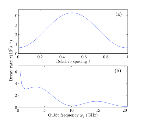
Figure 4: Plot of the decay rate of a function of (a) the relative spacing $\ell$ and (b) the qubit frequency $\omega_{\mathrm{q}}$.

Using Eq. (40) for $|\mathfrak{s}(k_{\mathrm{q}})|$ and $|\mathfrak{s}(0)|$, the decay rate as a function of both $\ell$ and $\omega_{\mathrm{q}}$ is plotted in Fig. 4. The plot in part (a) shows a symmetric decay rate about the qubit spacing. At the two limiting ends with $\ell=0$ and $\ell=1$ where the coupling factor $\cos(j\pi\ell)$ falls back to 1, all qubits in the quasi-lattice are maximally coupled to the cavity field. Under such a circumstance, each qubit is equally excited and has the least probability to reabsorb radiated photons, resulting in a minimal probability of spontaneous radiation and the slowest decay. On the contrary, at the middle ground with $\ell=1/2$, only half of the qubits (the qubits at the antinodes) are coupled to the cavity field while the other half (the qubits at the nodes) are never excited by the cavity photon. The latter half are all open to reabsorbed the photons emitted from the former half, maximizing the likelihood of spontaneous emission across the qubits and giving the largest decay rate for the quasi-lattice.

The inhomogeneous coupling here unevenly excites every other qubit. When the population of every other qubit is fully inverted, the spin moment $m$ of the entire quasi-lattice would become zero. Following Dicke’s argument dicke54 , this results in a radiated intensity proportional to $\frac{N}{2}(\frac{N}{2}+1)$, i.e. superradiance. The prediction of a strong but short radiation pulse matches the largest decay rate predicted here.

From the plot in Fig. 4(b), we see the decay also matches with the selective radiation we derived in Sec. IIIA. At the quasi-period $K$ of Eq. (27) or half of it, the quasi-lattice are resonant with the cavity where the emitted photons have the highest probability of being trapped in the cavity and reabsorbed by the quasi-lattice, giving a minimal decay rate. At the non-resonant cases, the photons emitting into the waveguide increase and thus the decay increases.

V Conclusion and discussions

We study the formation of polaritons in a quasi-lattice of superconducting qubits, that is a linear chain of qubits with inhomogeneous coupling to a cavity field in a stripline resonator. We show that the radiation of the quasi-lattice polariton is different from that of an atomic lattice: the radiation amplitude can be either enhanced or lowered over the radiation frequency, depending on the resonance between the polariton and the radiated photon. This amplitude shows a quasi-periodicity determined by the structure of the quasi-lattice. Further, we find that the decay of the polariton excited states also depends on the structure of the quasi-lattice, in particular its spacing $\ell$ between the qubits relative to the cavity wavelength. The decay obtains its maximum when the qubits in the quasi-lattice are alternatively excited by the cavity field. These unique features demonstrate the distinction of the mesocopic nature of superconducting qubit systems as opposed to the microscopic atoms they emulate.

In addition, since superconducting qubit circuits have played a great role in the development of quantum computation, the ability to filter quantum signals selectively using a set of such qubits will benefit the designs of sophisticated processing devices for quantum signals. For example, when the qubits are replaced by three-level systems fabricated on superconducting circuits, sophisticated photon detectors can be implemented romero09 ; peropadre11 . Further, it was shown coherent photon transport can be realized on coplanar waveguides with embedded atoms shen05 . Henceforth, if we regard the quasi-lattice as a mediating device in the coplanar waveguide, complex control over photon transports by the structure of the quasi-lattice is very likely to occur.

Overall, the study we present here aims to lay the groundwork for the physics of many-qubit systems in a circuit cavity. We expect that more interesting physical phenomena will be discovered when more variables are added to the system, especially those quantum optical effects emulatable in a superconducting qubit circuit jqyou11 . It was found that, for example, a single qubit can be dressed by the cavity field to form an effective three-level system. When a strong coherent field is added to drive this three-level system, tunable electromagnetically induced transparency and absorption can be achieved due to the tunable dressed relaxations ian10 . We can resonably expect that the situation would be much more complex if the quasi-lattice is driven by the coherent field. For example, while the current experiments only demonstrate the stimulated emission on a single qubit astafiev07 ; astafiev10 similar to those in atomic optics, the extension to a quasi-lattice of qubits might lead to new patterns of stimulated emission. And the quasi-lattice of qubits is experimentally accessible using current technologies.

Another direction worth investigating is to consider that the eigenfrequencies of the qubits are also non-uniform. In this case, the deformed SU(2) algebra formed by the quasi-lattice would need further generalizations. One way to include this non-uniformity into the deformed algebra is through the statistical approach similar to what we have adopted for quasi-lattices with non-uniform spacings in Ref. ian13 , where the variations are measured by a pair of mean variance. These two parameters can then be included in the deformation factor that describes the quasi-lattice. We hope to extend this consideration and give a more detailed study in a future paper.

Appendix A Matrix elements of the excitation operator

To verify that the diagonal elements of $S_{+}$ in the polariton basis vanish, consider for arbitrary $u$

$$[S_{+}]_{uu} = \left\langle u,r\right|S_{+}\left|u,r\right\rangle$$

$$= \sum_{m,n}c_{m}^{\ast}c_{n}\left\langle m;r,u-m\right|S_{+}\left|n;r,u-n\right\rangle$$

$$= \sum_{m,n}c_{m}^{\ast}c_{n}\sqrt{\mathfrak{f}(r-u+n)(r+u-n+1)}$$

$$\times\left\langle m;r,u-m|n;u-n+1\right\rangle$$

where the inner product in the last line equals to the Kronecker product $\delta_{mn}\delta_{u-m,u-n+1}$. Since $m$ cannot simultaneously equal to both $n$ and $n+1$, the diagonal elements $[S_{+}]_{uu}=0$ for any $u$. Similar arguments also apply to the conjugate $S_{-}$.

For the non-diagonal elements with $u\neq v$, we expand the bra’s and ket’s using Eq. (13) to get

$$[S_{+}]_{uv}= \left\langle u,r\right|S_{+}\left|v,r\right\rangle$$

$$= \sum_{m,n}c_{m}^{(u)\ast}c_{n}^{(v)}\left\langle r,u-m;m\right|S_{+}\left|r,v-n;n\right\rangle$$

$$= \sum_{m,n}c_{m}^{(u)\ast}c_{n}^{(v)}\sqrt{\mathfrak{f}(r-v+n)(r+v-n+1)}$$

$$\times\delta_{m,n}\delta_{u-m,v-n+1}$$

$$= \sum_{n}c_{n}^{(u)\ast}c_{n}^{(v)}\sqrt{\mathfrak{f}(r-v+n)(r+v-n+1)}\delta_{u,v+1}.$$

The last line in the expansion demands that except for the first off-diagonal, all other off-diagonal elements vanish, thus giving the expression in Eq. (21). Following the same logic, the lowering ladder operator has also only the first off-diagonal elements.

$$[S_{-}]_{uv}= \left\langle u,r\right|S_{-}\left|v,r\right\rangle$$

$$= \sum_{m,n}c_{m}^{(u)\ast}c_{n}^{(v)}\left\langle r,u-m;m\right|S_{-}\left|r,v-n;n\right\rangle$$

$$= \sum_{m,n}c_{m}^{(u)\ast}c_{n}^{(v)}\sqrt{\mathfrak{f}(r+v-n)(r-v+n+1)}$$

$$\times\delta_{m,n}\delta_{u-m,v-n-1}$$

$$= \sum_{n}c_{n}^{(u)\ast}c_{n}^{(v)}\sqrt{\mathfrak{f}(r+v-n)(r-v+n+1)}\delta_{u,v-1},$$

giving the expression of Eq. (22).

Appendix B Commutation relations of the deformed operators

For the operators $\{S_{z},S_{+},S_{-}\}$ of the collective excitations on the quasi-lattice, their structure of deformed SU(2) algebra breaks one of the commutation relation: $[S_{+},S_{-}]\neq 2S_{z}$. However, the other two commutation relations are preserved:

$$[S_{z},S_{\pm}]=\pm S_{\pm}.$$

See App. A of Ref. ian12 for a detailed derivation and discussion.

In the transformed polariton basis, $S_{+}$ is expressed using Eq. (19) and Eq. (21). We can see the commutation relation becomes

$$\left[\sum_{u}\Omega_{u}\left|u,r\right\rangle\left\langle u,r\right|,S_{+}\right]$$

$$= \sum_{u,v}\Omega_{u}[S_{+}]_{v,v-1}\left[\left|u,r\right\rangle\left\langle v-1,r\right|\delta_{u,v}-\left|v,r\right\rangle\left\langle u,r\right|\delta_{v-1,u}\right]$$

$$= \sum_{u}\Omega_{u}\biggl{\{}[S_{+}]_{u,u-1}\left|u,r\right\rangle\left\langle u-1,r\right|$$

$$-[S_{+}]_{u+1,u}\left|u+1,r\right\rangle\left\langle u,r\right|\biggr{\}}$$

$$= \sum_{u}(\Omega_{u}-\Omega_{u-1})[S_{+}]_{u,u-1}\left|u,r\right\rangle\left\langle u-1,r\right|$$

$$= \omega_{\mathrm{q}}S_{+}+\sum_{u}(\varepsilon_{u}-\varepsilon_{u-1})[S_{+}]_{u,u-1}\left|u,r\right\rangle\left\langle u-1,r\right|,$$

where we have broken up each polariton eigenfrequency $\Omega_{u}$ into two parts: the excitation energy part $u\omega_{\mathrm{q}}$ and the lattice-photon interaction part $\varepsilon_{u}$ ian13 . The latter accounts for fine splittings due to the interaction of each cluster energy level $u\omega_{\mathrm{q}}$. It is determined by the coupling strength $\eta$ and the detuning $\Delta\omega$. For low excitation number $u$, its value is less affected by the number $u$ and the difference between two consecutive ones is minimal as compared to $\omega_{\mathrm{q}}$, i.e. $\varepsilon_{u}-\varepsilon_{u-1}\ll\omega_{\mathrm{q}}$.

Therefore, we can consider the commutation relation for $S_{+}$ still preserves after the transformation to the polariton basis. Normal Baker-Hausdorff formula can then be applied to obtain the Hamiltonian in the interaction picture as in Eq. (28).

Appendix C Convergence in Wigner-Weisskopf approximation

First, substituting the expression of $g_{k}^{2}$ into Eq. (36), we have the equation of motion

$$\frac{\mathrm{d}}{\mathrm{d}t}\alpha(t)=\alpha(t)\frac{\lambda_{\mathrm{C}}k_{\mathrm{q}}^{2}\mu^{2}}{4\pi\epsilon V}\left[\mathscr{P}\negthickspace\int\negthickspace\mathrm{d}k\frac{|\mathfrak{s}(k)|^{2}}{ik(k-k_{\mathrm{q}})}-\frac{\pi}{k_{\mathrm{q}}}|\mathfrak{s}(k_{\mathrm{q}})|^{2}\right].$$ (42)

When extending the integration variable $k$ to the complex plane of variable $z$, the principal value avoids the singularity at $z=0$, effectively setting the integral as the difference of two integrals

$$\mathscr{P}\int\mathrm{d}z=\lim_{\epsilon\to 0}\left[\int_{-\infty}^{-\epsilon}+\int_{\epsilon}^{\infty}\right]\mathrm{d}z=\oint\mathrm{d}z-\int_{\mathrm{sc}}\mathrm{d}z$$ (43)

where $\mathrm{\oint}$ indicates a closed contour integral with an infinite-radius arc in the upper complex plane and $\int_{\mathrm{sc}}$ indicates a path integral along a small semi-circle over $z=0$.

To verify the path along the infinite-radius arc does not contribute to the integration, we can first decompose the fraction to have

$$\int\mathrm{d}k\frac{|\mathfrak{s}(k)|^{2}}{ik(k-k_{\mathrm{q}})}=\frac{i}{k_{\mathrm{q}}}\int\mathrm{d}k\left[\frac{|\mathfrak{s}(k)|^{2}}{k}-\frac{|\mathfrak{s}(k)|^{2}}{k-k_{\mathrm{q}}}\right]$$ (44)

where $|\mathfrak{s}(k)|^{2}$ is a sum of $|\chi_{l}(k)|^{2}$. It is not necessary to prove the convergence of the integral from $\chi_{l}(k)$ directly. Since $\chi_{l}(k)$ is a finite sum of the exponential $e^{ikr_{j}}$, we can simply verify that, in the modulus $|\chi_{l}(k)|^{2}$, each product term $e^{ik(r_{j}-r_{j^{\prime}})}$ be convergent with the integration along the infinite-radius arc. That is,

$$\int\mathrm{d}k\frac{e^{ik(j-j^{\prime})L_{\mathrm{q}}}}{k} = \int_{\mathrm{arc}}\mathrm{d}z\frac{e^{iz}}{z}$$

$$= \lim_{|z|\to\infty}\int_{\mathrm{0}}^{\pi}\mathrm{d}\theta|z|ie^{i\theta}\frac{\exp\{i|z|e^{i\theta}\}}{|z|e^{i\theta}}$$

$$= \lim_{|z|\to\infty}i\int_{\mathrm{0}}^{\pi}\mathrm{d}\theta\left[e^{i|z|\cos\theta}e^{-|z|\sin\theta}\right]$$

For Hölder’s inequality, we see the modulus is upper-bounded

$$\left|\int_{\mathrm{arc}}\right| \leq \lim_{|z|\to\infty}\int_{\mathrm{0}}^{\pi}\mathrm{d}\theta\left|e^{i|z|\cos\theta}\right|\cdot\left|e^{-|z|\sin\theta}\right|$$

$$= \lim_{|z|\to\infty}\int_{\mathrm{0}}^{\pi}\mathrm{d}\theta\left|e^{-|z|\sin\theta}\right|$$

$$= \lim_{|z|\to\infty}2\int_{\mathrm{0}}^{\pi/2}\mathrm{d}\theta e^{-|z|\sin\theta}.$$

Furthermore, the integral vanishes when the limit is taken. Observe that for $\theta\in(0,\pi/2)$, the exponential function above is monotonically non-decreasing. Since the sine function in the first quadrant is always greater than the diagonal line, i.e. $|z|\sin\theta>|z|\frac{\theta}{\pi/2}$, by exponentiating both sides, we have

$$e^{-|z|\sin\theta}<e^{-2|z|\theta/\pi}.$$

The right hand side can be easily integrated such that

$$\left|\int_{\mathrm{arc}}\right| < \lim_{|z|\to\infty}2\int_{0}^{\pi/2}e^{-2|z|\theta/\pi}$$

$$= \lim_{|z|\to\infty}\frac{\pi}{|z|}(1-e^{-|z|}).$$

When the limit is taken, we see the path integral vanishes.

For the second term in Eq. (44), we see it is identical to the first term up to an exponential factor:

$$\int\mathrm{d}k\frac{e^{ik(j-j^{\prime})L_{\mathrm{q}}}}{k-k_{\mathrm{q}}}=e^{ik_{\mathrm{q}}(j-j^{\prime})L_{\mathrm{q}}}\int_{\mathrm{arc}}\mathrm{d}z\frac{e^{iz}}{z}$$

where $z=k-k_{\mathrm{q}}$, i.e. $k$ is extended to the complex with a translated origin at $k=k_{\mathrm{q}}$. Similarly, it will also vanish at $|z|\to\infty$. The proof that the contour integral in Eq. (43) vanishes is now completed and the only contribution to the principal value is the second integral at $|z|\to 0$.

For this integral along a small semicircle above the singularities, we compute the contribution by each exponential in $|\mathfrak{s}(k)|^{2}$. For the first term in Eq. (44),

$$\int_{\mathrm{sc}}\mathrm{d}z\frac{e^{iz}}{z}=\lim_{|z|\to 0}i\int_{\mathrm{\pi}}^{0}\mathrm{d}\theta\left[e^{i|z|\cos\theta}e^{-|z|\sin\theta}\right]=-i\pi.$$

The second term has the identical result with the same extra exponential factor as above, hence

$$\int\mathrm{d}k\frac{e^{ik(r_{j}-r_{j^{\prime}})}}{ik(k-k_{\mathrm{q}})}=\frac{\pi}{k_{\mathrm{q}}}\left[1-e^{ik_{\mathrm{q}}(j-j^{\prime})L_{\mathrm{q}}}\right]$$

For the total contribution of $|\mathfrak{s}(k)|^{2}$, we then have

$$\mathscr{P}\int\mathrm{d}k\frac{|\mathfrak{s}(k)|^{2}}{ik(k-k_{\mathrm{q}})}$$

$$= \frac{\pi}{N^{2}k_{\mathrm{q}}}\sum_{Nl,Nl^{\prime}}^{N-1}\sum_{j,j^{\prime}}^{N-1}\cos(j\pi l)\cos(j\pi l^{\prime})\left[1-e^{ik_{\mathrm{q}}(j-j^{\prime})L_{\mathrm{q}}}\right]$$

$$[S_{l,+}]_{10}[S_{l^{\prime},-}]_{01}$$

$$= \frac{\pi}{N^{2}k_{\mathrm{q}}}\sum_{Nl,Nl^{\prime}}^{N-1}\left[\chi_{l}(0)\chi_{l^{\prime}}(0)-\chi_{l}(k_{\mathrm{q}})\chi_{l^{\prime}}^{\ast}(k_{\mathrm{q}})\right][S_{l,+}]_{10}[S_{l^{\prime},-}]_{01}$$

$$= \frac{\pi}{k_{\mathrm{q}}}\left\{|\mathfrak{s}(0)|^{2}-|\mathfrak{s}(k_{\mathrm{q}})|^{2}\right\}$$

Plugging the above result into Eq. (42), we see the terms about $k_{\mathrm{q}}$ will cancel out and arrive at the equation of motion (38).

Appendix D Deriving the coefficients for one-excitation in $N=4$ quasi-lattice

For a $N=4$ quasi-lattice, we have the total spin $r=2$ and the magnetic moment $m\in\{-2,-1,0,1,2\}$. Since we confine ourselves to the discussion of the ground and the first excited state, i.e. the excitation number $u$ being $-2$ and $-1$, respectively, there are three possible combinations of $n$ and $m$ that satisfies $n+m=u$. For the ground state $u=-2$, we have one configuration in the expansion of Eq. (13), so

$$c_{0}^{(-2)}=1.$$

For the coefficients in the expansion of the first excited polariton state, we can either plugging in the numbers into Eq. (14) or follow the routine of finding a set of difference equations ian12 . In this case, the latter is simpler and we have

$$c_{1}^{(-1)} = \frac{\varepsilon}{2\eta\sqrt{\mathfrak{f}}}c_{0}^{(-1)},$$

$$0 = \frac{\varepsilon-\Delta\omega}{\eta\sqrt{2\mathfrak{f}}}c_{1}^{(-1)}-\sqrt{2}c_{0}^{(-1)}.$$

Combining these two equations, we find a quadratic equation for $\varepsilon$

$$\varepsilon^{2}-\Delta\omega\varepsilon-4\eta^{2}\mathfrak{f}=0,$$

the solution of which is given in Eq. (41).

Further, using the normality condition for the superposition coefficients, we get

$$c_{0}^{(-1)} = \sqrt{\frac{4\eta^{2}\mathfrak{f}}{\varepsilon^{2}+4\eta^{2}\mathfrak{f}}},$$

$$c_{1}^{(-1)} = \sqrt{\frac{\varepsilon^{2}}{\varepsilon^{2}+4\eta^{2}\mathfrak{f}}}.$$

Then, substituting the coefficients into the expression $2\sqrt{\mathfrak{f}}c_{0}^{(-1)}c_{0}^{(-2)}$ for $[S_{l,+}]$, we arrive at Eq. (40).

References

- (1) J. Clarke and F. K. Wilhelm, Nature 453, 1031 (2008).
- (2) A. Wallraff, D. I. Schuster, A. Blais, L. Frunzio, R.-S. Huang, J. Majer, S. Kumar, S. M. Girvin, and R. J. Schoelkopf, Nature 431, 162 (2004).
- (3) J. Majer, J. M. Chow, J. M. Gambetta, J. Koch, B. R. Johnson, J. A. Schreier, L. Frunzio, D. I. Schuster, A. A. Houck, A. Wallraff, A. Blais, M. H. Devoret, S. M. Girvin, and R. J. Schoelkopf, Nature 449, 443 (2007).
- (4) A. Blais, R.-S. Huang, A. Wallraff, S. M. Girvin, and R. J. Schoelkopf, Phys. Rev. A 69, 062320 (2004).
- (5) J. Q. You and F. Nori, Nature 474, 589 (2011).
- (6) I. Buluta and F. Nori, Science 326, 108 (2009).
- (7) M. Tavis and F. W. Cummings, Phys. Rev. 170, 379 (1968).
- (8) H. Ian, Y.X. Liu, and F. Nori, Phys. Rev. A 85, 053833 (2012).
- (9) H. Ian, arXiv:1306.2757 (2013).
- (10) C.-P. Sun and H.-C. Fu, J. Phys. A: Math. Gen. 22, L983 (1989).
- (11) R. H. Dicke, Phys. Rev. 93, 99 (1954).
- (12) V. Ernst and P. Stehle, Phys. Rev. 176, 1456 (1968).
- (13) J. Knoester and S. Mukamel, Phys. Rev. A 40, 7065 (1989).
- (14) J. Keeling, F. M. Marchetti, M. H. Szymańska, and P. B. Littlewood, Semicond. Sci. Technol. 22, R1 (2007).
- (15) V. Savona, Z. Hradil, A. Quattropani, and P. Schwendimann, Phys. Rev. B 49, 8774 (1994).
- (16) M. O. Scully, E. S. Fry, C. H. R. Ooi, and K. Wodkiewicz, Phys. Rev. Lett. 96, 010501 (2006).
- (17) A. A. Svidzinsky, J.-T. Chang, and M. O. Scully, Phys. Rev. A 81, 053821 (2010).
- (18) A. A. Svidzinsky, Phys. Rev. A 85, 013821 (2012).
- (19) N. E. Rehler and J. H. Eberly, Phys. Rev. A 3, 1735 (1971).
- (20) J. C. MacGillivray and M. S. Feld, Phys. Rev. A 14, 1169 (1976).
- (21) E. Ressayre and A. Tallet, Phys. Rev. A 15, 2410 (1977).
- (22) R. Bonifacio and L. A. Lugiato, Phys. Rev. A 11, 1507 (1975).
- (23) R. Glauder and F. Haake, Phys. Lett. A 68, 29 (1978).
- (24) D. Polder, M. F. H. Schuurmans, and Q. H. F. Vrehen, Phys. Rev. A 19, 1192 (1979).
- (25) J. M. Fink, R. Bianchetti, M. Baur, M. Göppl, L. Steffen, S. Filipp, P. J. Leek, A. Blais, and A. Wallraff, Phys. Rev. Lett. 103, 083601 (2009).
- (26) P. Macha, G. Oelsner, J.-M. Reiner, M. Marthaler, S. André, G. Schön, U. Huebner, H.-G. Meyer, E. Il’ichev, and A. V. Ustinov, arXiv:1309.5268 (2013).
- (27) S. De Liberato, Phys. Rev. Lett. 112, 016401 (2014).
- (28) P. Nataf and C. Ciuti, Nat Commun 1, 72 (2010).
- (29) O. Viehmann, J. von Delft, and F. Marquardt, Phys. Rev. Lett. 107, 113602 (2011).
- (30) C. P. Sun, Y. Li, and X. F. Liu, Phys. Rev. Lett. 91, 147903 (2003).
- (31) M. J. Stephen, The Journal of Chemical Physics 40, 669 (1964).
- (32) C. Cohen-Tannoudji, J. Dupont-Roc, and G. Grynberg, Atom-Photon Interactions: Basic Processes and Applications (Wiley, 1998).
- (33) L. Mandel and E. Wolf, Optical Coherence and Quantum Optics (Cambridge University Press, 1995).
- (34) G. Romero, J. J. Garcia-Ripoll, and E. Solano, Phys. Rev. Lett. 102, 173602 (2009).
- (35) B. Peropadre, G. Romero, G. Johansson, C. M. Wilson, E. Solano, and J. J. Garcia-Ripoll, Phys. Rev. A 84, 063834 (2011).
- (36) J. T. Shen and S. Fan, Opt. Lett. 30, 2001 (2005).
- (37) H. Ian, Y.X. Liu, and F. Nori, Phys. Rev. A 81, 063823 (2010).
- (38) O. Astafiev, K. Inomata, A. O. Niskanen, T. Yamamoto, Y. A. Pashkin, Y. Nakamura, and J. S. Tsai, Nature 449, 588 (2007).
- (39) O. Astafiev, A. M. Zagoskin, A. A. Abdumalikov, Y. A. Pashkin, T. Yamamoto, K. Inomata, Y. Nakamura, and J. S. Tsai, Science 327, 840 (2010).