Using Volcano Plots and Regularized-Chi Statistics in Genetic Association Studies

Abstract

Labor intensive experiments are typically required to identify the causal disease variants from a list of disease associated variants in the genome. For designing such experiments, candidate variants are ranked by their strength of genetic association with the disease. However, the two commonly used measures of genetic association, the odds-ratio (OR) and $p$-value, may rank variants in different order. To integrate these two measures into a single analysis, here we transfer the volcano plot methodology from gene expression analysis to genetic association studies. In its original setting, volcano plots are scatter plots of fold-change and $t$-test statistic (or $-$log of the $p$-value), with the latter being more sensitive to sample size. In genetic association studies, the OR and Pearson’s chi-square statistic (or equivalently its square root, chi; or the standardized log(OR)) can be analogously used in a volcano plot, allowing for their visual inspection. Moreover, the geometric interpretation of these plots leads to an intuitive method for filtering results by a combination of both OR and chi-square statistic, which we term “regularized-chi”. This method selects associated markers by a smooth curve in the volcano plot instead of the right-angled lines which corresponds to independent cutoffs for OR and chi-square statistic. The regularized-chi incorporates relatively more signals from variants with lower minor-allele-frequencies than chi-square test statistic. As rare variants tend to have stronger functional effects, regularized-chi is better suited to the task of prioritization of candidate genes.

Keywords: volcano plot; regularized-chi; genetic association analysis; rare variants; SNPs; type-2 diabetes;

Introduction

Volcano plots are graphical tools that are commonly used in the analysis of mRNA expression levels as obtained from microarray technology (Jin et al., 2001, Cui and Churchill, 2003, Li, 2012). In principle, volcano plots are scatter plots, with each point representing a probe set or a gene, and the $x$-coordinate being the (log) fold-change (FC) and $y$ being the $t$-statistic or $-\log_{10}$ of the $p$-value from a $t$-test. The reason for the popularity of volcano plot in microarray data analysis is due to its simultaneous display of two, albeit correlated, pieces of information – fold-change and $t$-statistic. Ranking genes by fold-change and by $t$-test does not necessarily lead to the same order in the differential expressed gene list, and can give rise to different biological conclusions.

However, there is a fundamental relationship between log-fold-change and $t$-statistic: while $\log$(FC) is a measure of the magnitude of a “signal”, the $t$-statistic is approximately $\log$(FC) divided by its standard error, i.e., a signal-to-noise ratio (Zhang and Cao, 2009, Li, 2012). This means that the log(FC) is an unstandardized measure of differential expression, whereas $t$-statistic is a noise-level-adjusted standardized measure. The distinction between the two types of measures of differential expression has parallels to the long standing discussions in behavioral science, psychology, epidemiology, meta-analysis, and engineering under the theme of “effect size” (Cohen, 1988). As one possible strategy to address this issue, volcano plots display both measures simultaneously.

In genetic association study, there has been a similar issue on deciding which measure of association is more useful: odds-ratio (OR) or $\chi^{2}$ test (either the chi-square test statistic or the $p$-value from $\chi^{2}$ test) (Li, 2008). Currently, most association analyses apply a $\chi^{2}$ test as the primary single-nucleotide-polymorphism (SNP) selection criterion in the initial screening, and use the OR as a secondary measure in a re-examination. However, the distinction between the role of two measures and their connection has not always been explained. Because selecting candidate SNPs and regions from the first stage for the replication stage is of great practical importance, one would like to add more information in the screening stage. We believe the application of volcano plots can be beneficial towards this goal.

One particular advantage of volcano plot in microarray analysis is that it provides a natural context in addressing “joint gene filtering” (Zhang and Cao, 2009, Li, 2012), which are the measures of differential expressions using both log-FC and $t$-statistic. In comparison, the ad hoc selection criterion such as “FC $>1.5$, and $p$-value $<10^{-3}$” could be called “double gene filtering” (Zhang and Cao, 2009, Li, 2012). In a volcano plot, the discriminant lines for double filtering are right-angled lines formed by the vertical and the horizontal lines, whereas those in joint filtering are smooth curves. The well known significance analysis of microarray (SAM) (Tusher et al., 2001, Chu et al., 2007) has a discriminant line in the form of $y=c_{0}+c_{1}/tan(\theta)$, where $\theta$ is the angle between the $y$-axis and the line connecting the gene point and the plot origin, (Li, 2012).

Our goal in transferring volcano plots from expression analysis to genetic association analyses is to find SNP-filtering criteria that incorporate information from both OR and $\chi^{2}$ test results. This effort may help the prioritization of SNPs and chromosome regions in a genome-wide association study (Cantor et al., 2010). Prioritization of candidate genes has wide application in every “omics” field (Tranchevent et al., 2011, Moreau and Tranchevent 2012). Usually, the prioritization strategies rely on external information of gene products, such as protein-protein interaction (Pattin and Moore, 2009) and pathways (Chen et al., 2009, Wang et al., 2010, Peng et al., 2010). In contrast, our approach is purely statistical, with the underlying assumption that OR may provide more biological information than $\chi^{2}$-test $p$-value in a realistic setting (finite sample size and sample heterogeneity).

The questions that are discussed in this paper are as follows: (i) How does the minor allele frequency of markers appear in a volcano plot? (ii) How can one choose the penalty term in a regularized-chi statistic for genetic data, and is the choice of this term important? (iii) Do any other unstandardized and standardized measurements exist that may be used for $x$- and $y$-axes in the volcano plot, besides OR and $\chi^{2}$ test statistic?

Methods and Materials

Unstandardized and sample-size-insensitive measures of differential allele frequencies: Denote the $2\times 2$ allele count contingency table as $\{n_{ij}\}$ ($i,j$= 1,2) where row $i$ is the case ($i=1$) or control ($i=2$) label, and column $j$ is the minor ($j=1$) or major ($j=2$) allele label. The minor-allele-frequency (MAF) in the case (control) group is $p_{1}=n_{11}/(n_{11}+n_{12})=n_{11}/n_{1*}$ ($p_{2}=n_{21}/n_{2*}$). The major-allele-frequencies are $q_{1}=1-p_{1}$ ($q_{2}=1-p_{2}$) for the case (control) group.

One can define several “differential allele frequency” measures that are insensitive to the sample size, for instance, the odds-ratio (OR) which is defined as $n_{11}n_{22}/(n_{12}n_{21})$ or $p_{1}q_{2}/(p_{2}q_{1})$. It is well known that the log-transformed OR, $\log(OR)=\log(n_{11}n_{22})-\log(n_{12}n_{21})$, approximately follows a normal distribution (Woolf, 1955). Another unstandardized measure is the direct calculation of allele frequency difference between the case and control group: $d_{MAF}=p_{1}-p_{2}=n_{11}/n_{1*}-n_{21}/n_{2*}=(n_{11}n_{22}-n_{12}n_{21})/(n_{1*}n_{2*})$. Furthermore, Wright’s fixation index, $F_{st}=1-(p_{1}q_{1}+p_{2}q_{2})/(2\overline{p}\cdot\overline{q})=1-0.5n^{2}(n_{11}n_{12}/n_{1*}+n_{21}n_{22}/n_{2*})/(n_{*1}n_{*2})$ ($\overline{p}=(p_{1}+p_{2})/2,\overline{q}=(q_{1}+q_{2})/2=1-\overline{p}$) provides an unstandardized measure of differential allele frequency(Wright, 1951). $F_{st}$ is a measure of allele frequency difference between two subpopulations that is used in population genetics and estimates the proportion of variations explained by population stratification. Here we assume for simplicity the two subpopulations are case and control population, with a 50:50 mixing ratio.

Standardized and sample-size-sensitive measures of differential allele frequencies: As a standardized and sample-size sensitive measure of differential allele frequency, the $\chi^{2}$ statistic ($n=n_{**}=\sum_{ij}n_{ij}$) (e.g., (Yates, 1984, Suh and Li, 2007))

$$X^{2}=\frac{(n_{11}n_{22}-n_{12}n_{21})^{2}n}{n_{1*}n_{2*}n_{*1}n_{*2}}=n(p_{1}-p_{2})^{2}\frac{n_{1*}n_{2*}}{(p_{1}n_{1*}+p_{2}n_{2*})(q_{1}n_{1*}+q_{2}n_{2*})}$$ (1)

is clearly proportional to sample size $n$, in the asymptotic limit, given $p_{1}\neq p_{2}$. Alternatively, log-OR itself can be standardized by its standard error, $\log(OR)/SE(\log(OR))$, where (Woolf, 1955)

$$SE(\log(OR))=\sqrt{\frac{1}{n_{11}}+\frac{1}{n_{12}}+\frac{1}{n_{21}}+\frac{1}{n_{22}}}=\sqrt{\frac{1}{p_{1}q_{1}n_{1*}}+\frac{1}{p_{2}q_{2}n_{2*}}}.$$ (2)

The standardized $\log(OR)$ is of the form of a Wald statistic.

A SNP dataset for illustration: For illustration purpose, we first use a genotyping data of an autoimmune disease on one chromosome only (chromosome 6) with 809 cases and 505 controls (Freudenberg et al., 2011). The initial 38735 SNPs are reduced to 35855 SNPs by requiring that both the case and the control group to have at least one copy of the minor allele (which allele is the minor is defined by the control group). This removes many SNPs with minor allele frequency (MAF) less than 0.05, though many low-MAF SNPs remain. These data are used in Fig.1, Fig.2, and Fig.4.

Genome-wide association study (GWAS) case-control data for type 2 diabetes: We use The Wellcome Trust Case Control Consortium (WTCCC) data for the type 2 diabetes (T2D), with 1924 T2D cases and 2938 controls (The Wellcome Trust Case Control Consortium, 2007, Zeggini et al., 2007). Differing from several other autoimmune diseases including rheumatoid arthritis and type 1 diabetes, there is no major susceptibility locus in MHC region for type 2 diabetes. The genotyping was carried out by the Affymetrix GeneChip 500k array. There are 459,446 autosomal SNPs which had already passed a quality control (QC) procedure by WTCCC.

We impose a further filtering criterion: (i) $p$-value for testing unbiased typing ratio is larger than $10^{-4}$; (ii) $p$-value for testing Hardy-Weinberg equilibrium in both the control and the case group is larger than $10^{-4}$; (ii) MAF in both control and case group is larger than 0.005. This reduces the number of SNPs to 388,023 (84.45% of the original number).

Our MAF criterion is more relaxed than the 0.01 used in early analysis of these data (The Wellcome Trust Case Control Consortium, 2007, Zeggini et al., 2007), which leads to the inclusion of more rare variants. Although violation of HWE in the case group might be considered as part of disease signal (Feder et al., 1996, Nielsen et al., 1998, Song and Elston, 2006, Suh and Li, 2007, Li et al., 2008, Zheng et al., 2012), we noticed that in this data, it actually leads to SNPs with genotype distribution inconsistent between the case and the control group (e.g. the SNP rs3777582 on chromosome 6). This data is used in Fig.3.

Results

MAF of SNPs and angle in the volcano plot: To evaluate the role of the MAF of SNPs, we are using the volcano plots with $x=\log(OR)=\log(n_{11}n_{22})-\log(n_{12}n_{21})$, and $y=\log(OR)/SE(\log(OR))$. In microarray analysis, the angle $\theta$ between the $y$-axis and the line linking a gene dot and the origin is directly related to the standard error of the log-fold-change(Li, 2012), $\tan(\theta)=SE(\log(FC))$, and SE in turn is roughly the standard deviation of log-expression level divided by $\sqrt{n}$. Consequently, points closer to the $y$-axis are genes with low-variances. There is a parallel situation here by replacing fold-change with odds-ratio.

Using the formula in Eq.(2), we can write SE(log($OR$)) as (assuming equal number of case and control samples: $n_{1*}=n_{2*}=n/2$):

$$SE(\log(OR))=\sqrt{\frac{2}{n}}\sqrt{\frac{2+(1/p_{2}+1/q_{1})d_{MAF}}{p_{2}q_{1}(1+d_{MAF}/p_{2})(1+d_{MAF}/q_{1})}}$$ (3)

If MAF is approaching zero (e.g. $p_{2}\rightarrow 0$), then $SE(\log(OR))\sim 1/\sqrt{p_{2}}\rightarrow\infty$ and $\theta\rightarrow 90^{o}$. These are the points close to the $x$-axis which can have any OR values.

Fig.1 shows how the angle $\theta$ stratifies SNPs with different MAFs. The SNPs colored with red, orange, purple, blue correspond to those with control MAF $<0.01$, (0.01, 0.05), (0.05, 0.2), and $>0.2$. Note that the quality control step has already removed SNPs with very low MAFs and the control MAFs are greater than 0.00198. Also note that points with different colors may overlap, because according to Eq.(3), $\tan(\theta)$ is a function of both $p_{2}$ (control MAF) and $p_{1}$ (case MAF).

Regularized $\chi$-statistic: Later in this section, we will establish that standardized $\log(OR)$ is approximately equal to the square-root of $\chi^{2}$ statistic, or simply $\chi$. By following the similar definition of regularized $t$-statistic, or SAM for significance of analysis of microarray (Tusher et al., 2001, Chu et al., 2007), we define the regularized $\chi$-statistic as (through standardized $\log(OR)$):

$$\chi_{reg}=\frac{|\log(OR)|}{SE(\log(OR))+s_{0}}=\frac{|\log n_{11}n_{22}-\log n_{12}n_{21}|}{\sqrt{\frac{n_{1*}}{n_{11}n_{12}}+\frac{n_{2*}}{n_{21}n_{22}}}+s_{0}}=\frac{|\log p_{1}q_{2}-\log p_{2}q_{1}|}{\sqrt{\frac{1}{p_{1}q_{1}n_{1*}}+\frac{1}{p_{2}q_{2}n_{2*}}}+s_{0}}$$ (4)

If we use $i$ to index SNPs, $\chi_{reg,i}$ contains SNP-specific allele frequencies $(p_{1},p_{2})_{i}$, but $s_{0}$ is the same for all SNPs. The introduction of the constant $s_{0}$ makes the $\chi$-statistic more robust – less sensitive to chance fluctuation of SNP-specific standard error estimation.

Though not further used in this paper, we note that there are other ways to define a regularized test statistic. For example, we may use the definition of $\chi^{2}$-statistic and add an extra constant in the denominator (this is parallel to a proposed regularized $t$-test in microarray analysis (Baldi and Long, 2001)):

$$\chi^{2}_{reg}=\frac{(p_{1}-p_{2})^{2}}{\frac{(p_{1}n_{1*}+p_{2}n_{2*})(q_{1}n_{1*}+q_{2}n_{2*})}{nn_{1*}n_{2*}}+s_{0}^{2}}$$ (5)

where the first term in the denominator is approximately the variance of $p_{1}-p_{2}$; or

$$\chi^{\prime}_{reg}=\frac{|p_{1}-p_{2}|}{\sqrt{\frac{(p_{1}n_{1*}+p_{2}n_{2*})(q_{1}n_{1*}+q_{2}n_{2*})}{nn_{1*}n_{2*}}}+s_{0}}$$ (6)

where the first term in the denominator is approximately the SE of $p_{1}-p_{2}$.

If we select SNPs by the criterion $\chi_{reg}\geq c$, it is equivalent to(Li, 2012) $y=|\log(OR)|/SE=[|\log(OR)|/(SE+s_{0})]\cdot[(SE+s_{0})/SE]\geq c(1+s_{0}/\log(\theta))$. In other words, instead of the horizontal line, the discriminant line is a smooth curve which moves up as it is closer to the $y$-axis (Fig.1). The regularized-$\chi$ combines information from both $\chi^{2}$ test and OR.

The choice of $s_{0}$ in regularized $\chi$-statistic: The regularization constant $s_{0}$ in SAM for expression analysis is chosen to minimize the dependence of relative variation of the SAM statistic on the standard error (Tusher et al., 2001, Chu et al., 2007, Åstrand, 2008). The more detailed procedure in choosing $s_{0}$ in SAM is the following: genes are grouped into 100 bins by their percentile of standard errors; within each bin, the variability of the SAM statistic is measured by the median absolute deviation (MAD); the dependency of relative variation of MAD on bin is calculated by sd(MAD)/mean(MAD); the constant $s_{0}$ is chosen to minimize sd(MAD)/mean(MAD).

In Fig.2(A), we examine the MAD of 100 bins of SE values at different $s_{0}$’s: 10%, 90%, 95%, and 100% percentiles of SE. There are several observations: first, the non-robust behavior mainly occurs at bins with large SE’s. Second, in terms of absolute variation, the choice of $s_{0}=\max(SE)$ seems to lead to lowest variation. Third, even if the lowest absolute variation occurs at $s_{0}=\max(SE)$, because the averaged MAD level is low, it is unclear whether the relative variation is also low.

Fig.2(B) and (C) show indeed that the absolute variation of MAD decreases with $s_{0}$, but relative variation increases, for both the parametric and non-parametric version of the measure of variation (sd, MAD_bin for absolute variation, sd/mean, MAD_bin/median for relative variation). If the relative variation is considered, as in the original discussion of SAM, then the $s_{0}=\min(SE)$ would be chosen.

Here, we consider an alternative measure of the robustness by combining both absolute and relative variation of MAD’s. For all $s_{0}$ values, we rank absolute (and relative) variation from low to high; then we add these two ranks; the $s_{0}$ with the lowest total rank is the value we use to regularize $\chi$. From Fig.2(D), either the min(SE) or 3% or 4%-percentile of SE depending on whether the parametric or non-parametric measure is used. For non-parametric measure, one can see that the averaged rank is quite stable for all $s_{0}$ values.

The consequence of $s_{0}$ is illustrated in Fig.1. Four discriminant lines are shown for $\chi=|\log(OR)|/(SE+s_{0})=\chi_{0}$. The SNP filtering criterion is $\chi\geq\chi_{0}$. All four lines plus the horizontal line (or $s_{0}=0$) selects top 70 SNPs (the corresponding $p$-value for the unregularized $\chi^{2}$ test is $10^{-4}$). This can be accomplished by tuning $\chi_{0}$ as the same time when various $s_{0}$ values are chosen. It can be seen that with a small $s_{0}$ value (0% or 4% percentile), there is already a great change in the shape of discriminant line (from straight line to curve), and many SNPs with less significant $\chi^{2}$ test result but larger ORs will be selected. The discriminant line with large $s_{0}$ (e.g. 100% percentile) should probably be avoided because it is too different from a unregularized $\chi^{2}$ test.

Re-examination of a published genome-wide association studies (GWAS) result by regularized $\chi$-statistics: We draw the volcano plot for 388,023 SNPs (see the Methods and Materials section) from The Wellcome Trust Case Control Consortium type 2 diabetes data in Fig.3. The three strongest signals are from the gene TCF7L2 (chr10), KIAA1005 (chr16) and CDKAL1 (chr6), consistent with the report in Table 3 of (The Wellcome Trust Case Control Consortium, 2007). In the subsequent validation stage, TCF7L2 and KIAA1005 signal remains (Table 1 of (Zeggini et al., 2007)) whereas KIAA1005 is dropped from the top gene list.

Fig.3 shows strikingly that the top results in such a GWAS run are biased towards common variants, as these genes are located at the inner envelope with the highest possible MAFs (smallest $\theta$ angle values). We have added two more genes further down the list: TSPAN8 (chr12) and RBMS1 (chr2). Interestingly, there are SNPs on both sides of the gene TSPAN8, and there are also both positive (OR $>1$) and negative (OR $<1$) signals. More data on TSPAN8 was reported in (Zeggini et al., 2008), and the RBMS1 region has later been validated by more GWAS projects (Qi et al., 2010)

There are usually no published GWAS results for rare variants using the commercial genotyping arrays with the typical SNP density (e.g. 500k). To illustrate this in volcano plot, we highlight the two SNPs near the gene HAPLN1 (chr5) in Fig.3, whose rankings increase the most when regularized-$\chi$ is used. These two SNPs pass the Hardy-Weinberg equilibrium tests in control ($p$-value=0.7) as well as in case ($p$-values=0.47, 0.52), and they pass the differential typing test ($p$-value=0.31, 0.11), lacking an indication of bad typing quality. The MAF is increased from 0.0065 in control to 0.015 in case, with $\chi^{2}$-statistic of 20.36, 14.93 ($p$-values= 6$\times 10^{-6}$), 1$\times 10^{-4}$, and ORs 2.5, 2.2. However, these two SNPs would not have passed the filtering in the original WTCCC analysis because the MAF is lower than 0.01. Using volcano plot and regularized-$\chi$, these rare variants are easily highlighted and deserve further attention.

Other potential choices of $x$- and $y$-axis of volcano plots: Besides the log-odds-ratio, other candidate for the unstandardized variables for the $x$-axis include minor allele frequency difference $d_{MAF}$ and the fixation index $F_{st}$. The MAF difference $d_{MAF}=(n_{11}n_{22}-n_{12}n_{21})/(n_{1*}n_{2*})$ may look very different from $\log(OR)$, but under the null hypothesis (i.e. zero allele frequency difference), the two measures are related, because:

$$\log(OR)=\log\left(1+\frac{d_{MAF}}{p_{2}}\right)\left(1+\frac{d_{MAF}}{q_{1}}\right)\approx\frac{d_{MAF}}{p_{2}}+\frac{d_{MAF}}{q_{1}}+O(d_{MAF}^{2})=\frac{d_{MAF}}{(1-p_{1})p_{2}}+O(d_{MAF}^{2})$$ (7)

Thus, if $d_{MAF}$ is far from zero, there is no simple relationship between the two. Fig.4(A) shows the existence of two distinct branches in the $d_{MAF}$ vs. $\log(OR)$ scatter plot. The first branch is for rare-allele SNPs (low $p_{1},p_{2}$ value), which more or less trace the line $\log(OR)\sim p_{2}^{-1}d_{MAF}$. The second branch is for common alleles ($p_{1}\approx p_{2}\approx 0.5$), where $\log(OR)\sim 4d_{MAF}$. Both approximations can be obtained from Eq.(7). SNPs with low MAF are more likely to achieve high OR values, but never high $d_{MAF}$; whereas SNPs with common MAF tend to have large $d_{MAF}$, but only limited OR. Note that SNPs which rank high by $\chi^{2}$ test result shown in Fig.3 belong to the common variant branch, whereas those ranking relatively high in regularized-$\chi$ (Fig.3) tend to belong to the rare variant branch.

The fixation index $F_{st}$ is highly correlated with $\log(OR)$ (Fig.4(B)). Interestingly, points (SNPs) with different MAF values overlap with each other on Fig.4(B), thus not stratified by MAF (result not shown). It can be shown that

$$F_{st}=\frac{d_{MAF}^{2}}{(p_{1}+p_{2})(2-p_{1}-p_{2})},$$ (8)

so $F_{st}$ scales as the square of allele frequency differences.

Here we used the standardized $\log(OR)$ as the $y$-axis, but could instead also have used the $\chi^{2}$-statistic. In fact, the two are very similar (see Fig.4(C)), and both are expected to approximate a standard normal distribution. Fig.4(D) and Fig.1 show two versions of a volcano plot, with the former uses $\chi^{2}$ vs. $\log(OR)$, and second uses $\log(OR)/SE(\log(OR))$ vs. $\log(OR)$. The difference between the two is mostly due to the fact that $\chi^{2}$ is the square of a normally distributed variable, so that straight lines in Fig.1 become parabola in Fig.4(D).

Discussion

Like any graphical representation of data or analysis results, such as effect size vs. sample size in the funnel plot (Egger et al., 1997), true positive rate vs. false positive rate in receiver operating characteristic (ROC) curve (Swets and Pickett, 1982), etc., the introduction of volcano plot to the genetic association studies brings in new perspectives. The role of MAF in balancing test $p$-value and OR, and in the biased selection of variants in GWAS, can be easily concluded from the volcano plot.

The idea of regularized-$\chi$ is the same as that of regularized-$t$ (or SAM) in microarray analysis: the avoidance of over-confidence in the ability to exactly estimate variances. The consequence is that those SNPs (or genes in microarray data) with extremely good test result (due to low standard error estimations) – but mediocre signal strength – move down in the ranking list.

The goal of the current paper is to introduce the concept of regularized-$\chi$, whereas more details have to be worked out in future publications. For example, the choice of $s_{0}$ here is not based on a solid theoretical ground. However, the same comment may also be made on the SAM in microarray analysis. And we have shown that for $s_{0}$ being non-zero is more important than having a specific value. Also, we mainly focus on the effect of regularization on the ranking order of SNPs, thus the choice of the threshold value and the resulting distribution of type I and type II error rates has not been discussed.

Regularized-$\chi$ can be applied to published GWAS results even when only the summary statistics are available. We have known in Fig.4(C) that the square-root of $\chi^{2}$-statistic is approximately equal to the standardized $\log(OR)$, or $\log(OR)/SE(\log(OR))$. Consequently, SE(log(OR)) is equal to $\log(OR)/\sqrt{\chi^{2}}$. Even if we may not know the distribution of SE(log(OR)) for all SNPs when a publication only provides the top-ranking results, these SNPs tend to have lower value of SE(log(OR)); the minimum of them could be the $s_{0}$ value in defining regularized-$\chi$.

Unlike the regularized-$t$ in microarray analysis, in genetic association analysis we have a clear understanding of the cause for a low standard error. This can be seen from Fig.1 where the points/SNPs forming small angles with the $y$-axis, thus having low standard errors, are all common variants with higher MAFs. Indeed, common SNPs have more statistical power than rare variants, but the true disease susceptibility genes with low allele frequencies are likely to be missed if $p$-values are used as the filtering criterion. The purpose or consequence of regularized-$\chi$ then becomes clear: it puts the signal originating from rare variants as measured by OR in the context of common variant association signals.

On the practical side, this effect of regularized-$\chi$ to select rare variants can come in conflict with the quality control, because genotyping errors can be mistaken as rare variants. Points/SNPs with the lowest MAFs form the bottom layer of the envelope in Fig.1, and the only way these would pass the regularized-$\chi$ threshold is to have large OR values. In fact, the OR could be infinity when one of the allele count is zero (though in principle, it could be avoided by a Yate’s correction). As a result, requiring a minimum number of minor allele (in both case and control group) to be included in the dataset can be an effective way to exclude low-quality SNPs to be selected. However, as sample size increases and genotyping technology matures, this becomes less of a concern. Ultimately, appropriate filtering threshold for MAF depends on the genotyping technology (e.g. microarray versus exome sequencing) and its error rate.

It is well known that genetic association signals from rare variants using array-based genotyping data is difficult. With the low density (500k) SNPs and low number of samples, rare disease-gene-containing haplotype may not be tagged effectively. However, with the next-generation sequencing (NGS) data, rare variances are called with more confidence, and we expect the volcano plot could play an important role in the analysis of such data.

FIGURE CAPTIONS

Fig.1: Volcano plot of 38735 SNPs located in chromosome 6 for a GWAS for an autoimmune disease with 809 cases and 505 controls. The angle $\theta$ is related to the standard error of $\log(OR)$ by the equation: $\tan(\theta)=SE(\log(OR))$. The colors red, orange, purple,and blue label SNPs with control MAFs in the intervals of (0.00198, 0.01), (0.01, 0.05), (0.05,0.2), and (0.2, 0.5). The horizontal line corresponds to $\sqrt{\chi^{2}}=3.89$ or $p$-value equal to $10^{-4}$. The threshold $\chi\geq 3.89$ filters 70 SNPs. The threshold for regularized $\chi$ with $s_{0}=0.08$ (minimum of SE), $s_{0}=0.08049$ (4% percentile), $s_{0}=0.2194957$ (90% percentile), and $s_{0}=1.00086$ (maximum of SE) are also shown, where the $\chi_{0}$ ($\chi\geq\chi_{0}$) is chosen so that exactly 70 SNPs are filtered.

Fig.2: (A) MAD (median of absolute deviation) of regularized $\chi$’s in 100 bins of SE(log(OR))’s at 4 $s_{0}$ values: $s_{0}=0.081$ (10% percentile), $s_{0}=0.2194957$ (90% percentile), $s_{0}=0.344$ (95% percentile), and $s_{0}=1.00086$ (maximum or 100% percentile). (B) Two measures of absolute variation of MAD’s in (A) along bins: standard deviation (sd(MAD)) and median of absolute deviation (MAD_bin(MAD) multiplied by 1.4826), as a function of $s_{0}$. (C) Two measures of relative variation of MAD’s in (A) along bins: coefficient of variation (sd(MAD)/mean(MAD)) and MAD_bin(MAD)/median(MAD), as a function of $s_{0}$. (D) Sum of rank of absolute variation in (B) and rank of relative variation in (C) divided by 2. The ranking is from low to high values. The $x$-axis is the bin number for $s_{0}$’s.

Fig.3: The volcano plot for The Wellcome Trust Case Control Consortium (WTCCC)’s type 2 diabetes (T2D) data, with 1924 cases and 2938 controls. Only a small portion of the 388,023 SNPs are shown as the background, with those on the following genes are highlighted: TCF7L2 (chr10, blue), KIAA1005 (chr16, purple), CDKAL1 (chr6, green), RBMS1 (chr2, orange, on the negative branch), TSPAN8 (chr12, brown, on both positive and negative branch), and HAPLN1 (chr5, red, rare variant).

Fig.4: (A) Scatter plot of $d_{MAF}$ ($x$-axis) and $\log(OR)$ ($y$-axis). Points far away from the origin are not plotted. Points (SNPs) are stratified by MAF in control group: crosses for low MAF (MAF $<0.05$), circles for high MAF (MAF $>0.2$), with all other points represented by dots. The two straight lines seem to envelope all points: one with slope 4 which traces common-allele SNPs, and another with slope $1/\min(p_{2})$ which traces rare-allele SNPs. (B) Scatter plot of $F_{st}$ ($x$-axis) and $\log(OR)$ ($y$-axis). (C) scatter plot of square-root of $\chi^{2}$-statistics ($x$) and standardized $\log(SE)$ in absolute value, $|\log(OR)|/SE(\log(OR))$ ($y$). (D) volcano plot with $\log(OR)$ as $x$, $\chi^{2}$-statistics as $y$.

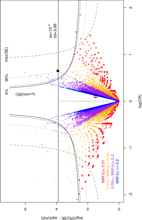
Figure 1:

Figure 2:

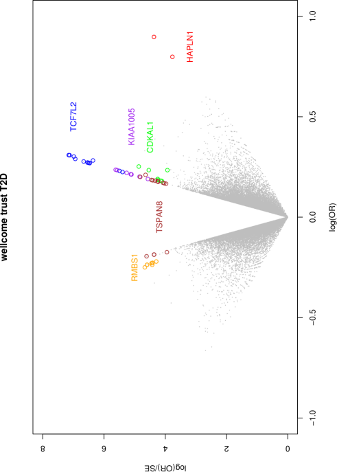
Figure 3:

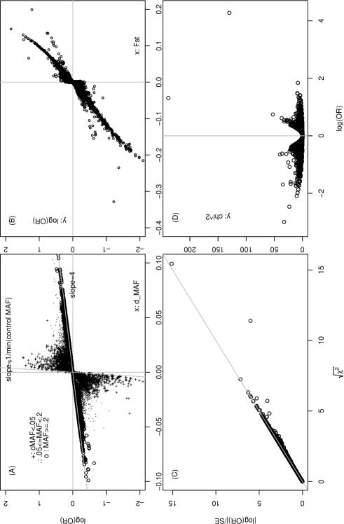
Figure 4:

References

- Åstrand, (2008) Åstrand M, 2008. Normalization and Differential Gene Expression Analysis of Microarray Data. Ph.D Thesis, Department of Mathematics, Chalmers University of Technology and Göteborg University.
- Baldi and Long, (2001) Baldi P, Long AD, 2001 A Bayesian framework for the analysis of microarray expression data: regularized t -test and statistical inferences of gene changes. Bioinformatics, 17, 509-519.
- Cantor et al., (2010) Cantor RM, Lange K, Sinshaimer JS, 2010. Prioritizing GWAS results: a review of statistical methods and recommendations for their application. Am. J. Hum. Genet., 86, 6-22.
- Chen et al., (2009) Chen L, Zhang L, Zhao Y, Xu L, Shang Y, Wang Q, Li W, Wang H, Li X, 2009. Prioritizing risk pathways: a novel association approach to searching for disease pathways fusing SNPs and pathways. Bioinformatics, 25, 237-242.
- Chu et al., (2007) Chu G, Narasimhan B, Tibshirani R, Tusher V, 2007. SAM: significance analysis of microarrays, users guide and technical document, v.3.0.
- Cohen, (1988) Cohen J, 1988. Statistical Power Analysis for the Behavioral Sciences, 2nd edition. Hillsdale, NJ, Lawrence Erlbaum Associates, Inc..
- Cui and Churchill, (2003) Cui X, Churchill GA, 2003. Statistical tests for differential expression in cDNA microarray experiments, Genome Biol., 4, 210.
- Feder et al., (1996) Feder JN, Gnirke A, Thomas W, et al., 1996. A novel MHC class I-like gene is mutated in patients with hereditary haemochromatosis. Nature Genet., 13, 399-408.
- Freudenberg et al., (2011) Freudenberg J, Lee HS, Han BG, et al., 2011. Genome-wide association study of rheumatoid arthritis in Koreans: population-specific loci as well as overlap with European susceptibility loci. Arthr. Rheum., 63, 884-893.
- Egger et al., (1997) Egger M, Smith GD, Schneider M, Minder C, 1997. Bias in meta-analysis detected by a simple, graphical test. BMJ, 315, 629-634.
- Jin et al., (2001) Jin W, Riley RM, Wolfinger RD, White KP, Passador-Gurgel G, Gibson G, 2001. The contributions of sex, genotype and age to transcriptional variance in Drosophila mel anogaster. Nature Genet., 29, 389-395.
- Li, (2008) Li W, 2008. Three lectures on case-control genetic association analysis. Brief. Bioinf., 9, 1-8.
- Li, (2012) Li W, 2012. Volcano plots in analyzing differential expressions with mRNA microarrays. J. Bioinf. Comp. Biol., 10, 1231002.
- Li et al., (2008) Li W, Suh YJ, Yang Y, 2008. Exploring case-control genetic association tests using phase diagram. Comp. Biol. Chem., 32, 391-399.
- Moreau and Tranchevent (2012) Moreau Y and Tranchevent LC, 2012. Computational tools for prioritizing candidate genes: boosting disease gene discovery. Nature Rev. Genet., 13, 523-536.
- Nielsen et al., (1998) Nielsen DM, Ehm MG, Weir BS, 1998. Detecting marker-disease association by testing for Hardy-Weinberg disequilibrium at a marker locus. Am. J. Hum. Genet., 63, 1531-1540.
- Pattin and Moore, (2009) Pattin KA, Moore JH, 2009. Role for protein–protein interaction databases in human genetics. Expert Rev. Proteomics, 6, 647-659.
- Peng et al., (2010) Peng G, Luo L, Siu H, Zhu Y, Hu P, Hong S, Zhao J, Zhou X, Reveille JD, Jin L, Amos CI, Xiong M, 2010. Gene and pathway-based second-wave analysis of genome-wide association studies. Euro. J. Hum. Genet., 18, 111-117.
- Qi et al., (2010) Qi L, Cornelis MC, Kraft P, et al., 2010. Genetic variants at 2q24 are associated with susceptibility to type 2 diabetes. Hum. Mol. Genet., 19, 2706-2715.
- Song and Elston, (2006) Song K, Elston RC, 206. A powerful method of combining measures of association and Hardy-Weinberg disequilibrium for fine-mapping in case-control studies. Stat. Med., 25, 105-126.
- Swets and Pickett, (1982) Swets JA and Pickett RM, 1982. Evaluation of Diagnostic Systems: Methods from Signal Detection Theory, Academic Press, New York.
- Suh and Li, (2007) Suh YJ, Li W, 2007. Genotype-based case-control analysis, violation of Hardy-Weinberg equilibrium, and phase diagrams. in Proc. 5th Asia-Pacific Bioinformatics Conf. Imperial College Press, London, pp.185-194.
- The Wellcome Trust Case Control Consortium, (2007) The Wellcome Trust Case Control Consortium, 2007. Genome-wide association study of 14,000 cases of seven common diseases and 3,000 shared controls. Nature, 447, 661-678.
- Tranchevent et al., (2011) Tranchevent LC, Capdevila FB, Nitsch D, de Moor B, de Causmaecker P, Moreau Y, 2011. A guide to web tools to prioritize candidate genes. Brief. Bioinf., 12,22-32.
- Tusher et al., (2001) Tusher VG, Tibshirani R, Chu G, 2001. Significance analysis of microarrays applied to the ionizing radiation response. Proc. Natl. Acad. Sci. , 98, 5116-5121.
- Wang et al., (2010) Wang K, Li M, Hakonarson H, 2010. Analysing biological pathways in genome-wide association studies. Nature Rev. Genet., 11, 843-854.
- Woolf, (1955) Woolf B, 1955. On estimating the relation between blood group and disease. Ann. Human. Genet., 19, 251-253.
- Wright, (1951) Wright S, 1951. The genetic structure of populations. Ann. Eugen., 15, 323-354.
- Yates, (1984) Yates F, 1984. Tests of significance for 2 x 2 contingency tables. J. Royal. Stat. Soc. SerA, 147, 426-463.
- Zeggini et al., (2008) Zeggini E, Scott LJ, Saxena R, et al., 2008. Meta-analysis of genome-wide association data and large-scale replication identifies additional susceptibility loci for type 2 diabetes. Nature Genet., 40, 638-645.
- Zeggini et al., (2007) Zeggini E, Weedon MN, Lindgren CM, et al., 2007. Replication of genome-wide association signals in UK samples reveals risk loci for type 2 diabetes. Science, 316, 1336-1341.
- Zhang and Cao, (2009) Zhang S, Cao J, 2009. A close examination of double filtering with fold change and t test in microarray analysis. BMC Bioinf., 10, 402.
- Zheng et al., (2012) Zheng G, Yang Y, Zhu X, Elston RC, 2012. Analysis of Genetic Association Studies. New York, Springer.