Also at: ]Jawaharlal Nehru Centre for Advanced Scientific Research, Jakkur, Bangalore, India.

Elliptical Tracers in Two-dimensional, Homogeneous, Isotropic Fluid Turbulence: the Statistics of Alignment, Rotation, and Nematic Order

Abstract

We study the statistical properties of orientation and rotation dynamics of elliptical tracer particles in two-dimensional, homogeneous and isotropic turbulence by direct numerical simulations. We consider both the cases in which the turbulent flow is generated by forcing at large and intermediate length scales. We show that the two cases are qualitatively different. For large-scale forcing, the spatial distribution of particle orientations forms large-scale structures, which are absent for intermediate-scale forcing. The alignment with the local directions of the flow is much weaker in the latter case than in the former. For intermediate-scale forcing, the statistics of rotation rates depends weakly on the Reynolds number and on the aspect ratio of particles. In contrast with what is observed in three-dimensional turbulence, in two dimensions the mean-square rotation rate increases as the aspect ratio increases.

The elucidation of the statistical properties of fluid turbulence is a problem of central importance in a variety of areas that include fluid dynamics, nonlinear dynamics, and non-equilibrium statistical mechanics MY75 ; frischbook ; BJPV98 ; PPR09 . Over the last decade or so, important advances have been made in developing an understanding of the statistical properties of homogeneous, isotropic turbulence in the Lagrangian framework FGV01 ; toschiannrev ; collinsannrev . Most of the studies in this framework, experimental, theoretical, and numerical, have used spherical or circular tracer particles in three and two dimensions (3D and 2D, respectively). The study of the dynamics of non-spherical particles in turbulent flows has applications in the simplest models for swimming micro-organisms KS11 , ice crystals in clouds CL94 , and fibers in the paper industry LSA11 . Recent work in 3D turbulent flows SK05 ; pumir11 ; toschi12 ; WK12 ; V13 ; CM13 ; GEM14 and in 2D low-Reynolds-number flows WBM09-10 ; voth11 has renewed interest in Lagrangian studies with anisotropic particles. We extend these studies to 2D, homogeneous and isotropic turbulence with elliptical tracer particles. Our study yields several interesting results, which have neither been obtained nor anticipated hitherto. We show that the dynamics of elliptical particles depends significantly on whether the fluid is forced at (A) large or (B) small length scales; the alignment of $\bm{p}$, the unit vector along the semi-major axis of an elliptical particle, and $\nabla\times\bm{\omega}$, where $\bm{\omega}$ is the vorticity, is more pronounced in case (A) than in case (B); and the statistics of the particle-rotation rate depends appreciably on the Reynolds number of the flow and the aspect ratio of the particles in case (A) but not in case (B). Moreover, we find important differences between the statistical properties of elliptical tracers in 2D turbulence and their counterparts for ellipsoidal particles in 3D turbulence. In 3D, $\bm{p}$ exhibits a strong alignment with $\bm{\omega}$ pumir11 , the mean-square-rotation rate of $\bm{p}$ decreases as the aspect ratio of particles increases toschi12 , and the autocorrelation function of $\bm{p}$ decays exponentially, with a correlation time increasing as a function of the Reynolds number pumir11 . By contrast, in 2D, we show that the alignment of $\bm{p}$ and $\nabla\times\bm{\omega}$ is much weaker than its analog in 3D, namely, the alignment of $\bm{p}$ and $\bm{\omega}$; in addition, the mean-square-rotation rate of $\bm{p}$ increases as the aspect ratio of particles increases. We thus extend significantly what is known about the differences between 2D and 3D turbulence frischbook ; L08 ; PPR09 ; BE12 .

Run	$N$	$\nu$	$\mu$	$f_{\mathrm{inj}}$	$k_{\mathrm{inj}}$	$\delta t$	$\eta$	$\lambda$	$Re_{\lambda}$	$T_{\mathrm{eddy}}$	$\tau_{\eta}$	$\tau_{S_{11}}$	$\tau_{S_{12}}$	$\tau_{\omega}$	$N_{p}$
A1	$2048$	$5\times 10^{-5}$	$0.01$	$1.9\times 10^{-6}$	$2$	$4.0\times 10^{-3}$	$3.3\times 10^{-2}$	$0.460$	$199$	$23.5$	$21.3$	$92.2$	$94.4$	$46.6$	$10^{4}$
B1	$2048$	$5\times 10^{-5}$	$0.01$	$7.8\times 10^{-3}$	$50$	$1.0\times 10^{-3}$	$3.8\times 10^{-3}$	$0.053$	$202$	$1.34$	$0.28$	$1.59\times 10^{-2}$	$1.61\times 10^{-2}$	$8.01\times 10^{-3}$	$10^{4}$
A2	$2048$	$5\times 10^{-5}$	$0.01$	$8\times 10^{-6}$	$2$	$2.0\times 10^{-3}$	$2.6\times 10^{-2}$	$0.470$	$382$	$14.7$	$12.0$	$24.7$	$24.1$	$12.2$	$10^{4}$
B2	$2048$	$5\times 10^{-5}$	$0.01$	$1.65\times 10^{-2}$	$50$	$5.0\times 10^{-4}$	$3.2\times 10^{-3}$	$0.063$	$385$	$1.37$	$0.21$	$8.66\times 10^{-3}$	$8.73\times 10^{-3}$	$4.35\times 10^{-3}$	$10^{4}$
A3	$2048$	$5\times 10^{-5}$	$0.01$	$1.5\times 10^{-5}$	$2$	$2.0\times 10^{-3}$	$2.0\times 10^{-2}$	$0.474$	$536$	$11.1$	$8.38$	$12.6$	$9.98$	$5.55$	$10^{4}$
B3	$2048$	$5\times 10^{-5}$	$0.01$	$2.5\times 10^{-2}$	$50$	$5.0\times 10^{-4}$	$3.0\times 10^{-3}$	$0.069$	$539$	$1.17$	$0.17$	$1.55\times 10^{-3}$	$1.56\times 10^{-3}$	$7.79\times 10^{-4}$	$10^{4}$

Table 1: The parameters for our DNS runs. Here, $\eta\equiv(\nu^{3}/\varepsilon)^{1/4}$ is the dissipation scale, $\lambda\equiv\sqrt{\nu\mathcal{E}/\varepsilon}$ the Taylor-microscale, $Re_{\lambda}=u_{rms}\lambda/\nu$ the Taylor-microscale Reynolds number, $T_{\mathrm{eddy}}\equiv\Sigma_{k}\frac{(E(k)/k)}{E(k)}/u_{rms}$ the eddy-turn-over time, and $\tau_{\eta}\equiv\sqrt{\nu/\varepsilon}$ the Kolmogorov time scale, where ${\mathcal{E}}\equiv\langle\frac{1}{2}|{\bm{u}(\bm{x}},t)|^{2}\rangle_{{\bm{x}},t}$, where $\langle\cdot\rangle_{{\bm{x}},t}$ denotes a space-time average, is the total kinetic energy of the flow, $u_{rms}$ is the root-mean-square velocity, $\varepsilon$ is the kinetic-energy dissipation rate, and $E(k)\equiv\sum_{k-1/2<k^{\prime}\leq k+1/2}k^{\prime 2}\langle|\widetilde{\psi}({\bm{k}^{\prime}},t)|^{2}\rangle_{t}$, where $\langle\cdot\rangle_{t}$ indicates a time average over the statistically steady state, is the fluid-energy spectrum. The Lagrangian correlation times of $S_{11}$, $S_{12}$, and $\omega$ are defined as $\tau_{S_{11}}\equiv\langle S_{11}^{2}\rangle^{-1}\int_{0}^{\infty}\langle S_{11}(t)S_{11}(0)\rangle\,dt$, $\tau_{S_{12}}\equiv\langle S_{12}^{2}\rangle^{-1}\int_{0}^{\infty}\langle S_{12}(t)S_{12}(0)\rangle\,dt$, and $\tau_{\omega}\equiv\langle\omega^{2}\rangle^{-1}\int_{0}^{\infty}\langle\omega(t)\omega(0)\rangle\,dt$, respectively.

The 2D, incompressible Navier–Stokes equations can be written in terms of the stream-function $\psi$ and the vorticity $\bm{\omega}=\nabla\times{\bm{u}}({\bm{x}},t)\equiv\omega{\hat{\bm{z}}}$, where ${\bm{u}}\equiv(-\partial_{y}\psi,\partial_{x}\psi)$ is the fluid velocity at the point ${\bm{x}}$ and time $t$, and $\hat{\bm{z}}$ is the unit normal to the fluid film:

$$D_{t}{\omega}=\nu\nabla^{2}{\omega}-\mu\omega+f_{\omega};~{}~{}~{}~{}\nabla^{2}{\psi}={\omega}.$$ (1)

Here $D_{t}\equiv\partial_{t}+{\bm{u}}\cdot\nabla$, the uniform solvent density $\rho=1$, $\mu$ is the coefficient of friction (which is always present in experimental fluid films PP10 ), and $\nu$ is the kinematic viscosity of the fluid. We use a zero-mean, Gaussian stochastic forcing with $\langle\tilde{f}_{\omega}(\bm{k})\tilde{f}_{\omega}(\bm{k}^{\prime})\rangle=A(\bm{k})\delta(\bm{k}+\bm{k}^{\prime}),$ where $A(\bm{k})=f_{\mathrm{inj}}$ if $|\bm{k}|=k_{\mathrm{inj}}$ and zero otherwise, the tilde denotes a spatial Fourier transform, and $k_{\mathrm{inj}}$ is the length of the energy-injection wave vector. The configuration of an elliptical particle is given by the position of its center of mass, $\bm{x}_{c}$, and by the axial unit vector $\bm{p}=(\cos\theta,\sin\theta)$ that specifies the orientation of the semi-major axis with respect to a fixed direction. The elliptical particles we consider are neutrally buoyant, of uniform composition, and much smaller than the viscous dissipation scale, so the velocity gradient is uniform over the size of a particle. In addition, we study suspensions that are sufficiently dilute for hydrodynamic particle–particle interactions to be disregarded. Under the above assumptions, $\bm{x}_{c}$ satisfies

$$\dot{\bm{x}}_{c}={\bm{u}}({\bm{x}}_{c}(t),t);$$ (2)

and the time evolution of the orientation is given by the Jeffery equation J22 , which reduces in a 2D, incompressible flow to the following one for the angle $\theta$:

$$\dot{\theta}=\textstyle\frac{1}{2}\omega+\gamma(\alpha)[\sin(2\theta)S_{11}-\cos(2\theta)S_{12}],$$ (3)

where $S_{ij}=(\partial_{i}u_{j}+\partial_{j}u_{i})/2$ are the components of the rate-of-strain tensor evaluated at $\bm{x}_{c}$, $\gamma(\alpha)\equiv(\alpha^{2}-1)/(\alpha^{2}+1)$, and $\alpha$ is the ratio of the lengths of the semi-major and semi-minor axes of the elliptical particle; $\gamma$ varies from 0 (circular disks) to 1 (thin rods).

Our direct numerical simulation (DNS) of Eqs. (1)-(3) uses periodic boundary conditions over a square domain with side $L=2\pi$, a pseudospectral method canuto88 with $N^{2}=2048^{2}$ collocation points, the $2/3$ dealiasing rule, and, for the time evolution, a second-order, exponential-time-differencing Runge–Kutta method cox02 ; PRMP11 . For the integration of Eq. (2), we use an Euler scheme, because, in one time step $\delta t$, a tracer particle crosses roughly one-tenth of a grid spacing. At off-lattice points, we evaluate the particle velocity from the Eulerian velocity field by using a bilinear-interpolation scheme num_recp . Finally, we integrate Eq. (3) by using an Euler scheme, with the same time step as for Eq. (2); and, at $t=0$, the orientation angles are uniformly distributed over $[0,2\pi]$. We track $N_{p}=10^{4}$ particles over time to obtain the statistics of particle alignment and rotation for $12$ different values of $0<\gamma\leq 1$. We collect data for averages only when our system has reached a non-equilibrium statistically steady state, i.e., for $t>20T_{\mathrm{eddy}}$, where $T_{\mathrm{eddy}}$ is the integral-scale eddy-turn-over time of the flow. The parameters used in our simulations are given in Table 1. Our study consists of two sets of simulations (A) and (B) at comparable values of $Re_{\lambda}$, the Taylor-microscale Reynolds numbers. In (A), the flow is forced at small $k_{\mathrm{inj}}$ (i.e., a large length scale); in (B), it is forced at an intermediate value of $k_{\mathrm{inj}}$ (i.e., an intermediate length scale); even in case (B) $k_{\mathrm{inj}}$ is small enough that the energy spectrum displays both a part with an inverse-energy cascade and a part with a forward cascade of enstrophy. We have also performed simulations at a lower resolution ($N=1024$) and obtained similar results, so our study do not suffer from finite-resolution effects.

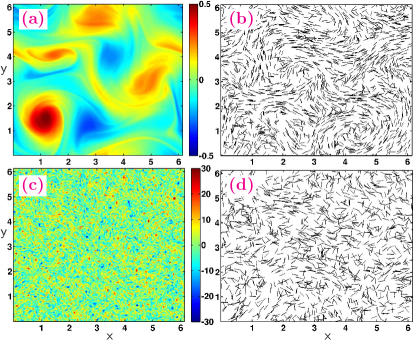
Figure 1: (Color online) (a) Pseudocolor plot of $\omega$ at $t=17.5$ for run A3; (b) particle positions and orientations at $t=17.5$ for run A3 and $\gamma=1$; (c) pseudocolor plot of $\omega$ at $t=17.5$ for run B3; (d) particle positions and orientations at $t=17.5$ for run B3 and $\gamma=1$. The number of particles shown in (b) and (d) is $2\times 10^{3}$. For the spatiotemporal evolution of these plots see Ref. SM .

In Fig. 1(a), we show a pseudocolor plot of $\omega$ for case (A) at a representative time in the statistically steady state; and Fig. 1(b) shows the positions and the orientations of particles at the same time; an elliptical particle is represented here by a black line whose center indicates $\bm{x}_{c}$ and whose orientation is that of $\bm{p}$. Analogous plots for case (B) are given in Figs. 1(c) and 1(d). Figure 1 suggests that the particle dynamics is qualitatively different in cases (A) and (B). In particular, in the former case, the orientation of particles is such that we see large-scale structures, which are absent in the latter case. To quantify this behavior, we study the statistics of the alignment of particles with the local directions of the flow.

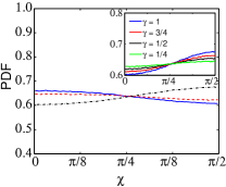
Figure 2: (Color online) PDFs of the angle between $\bm{p}$ and $\bm{\nabla}\times\bm{\omega}$. Left: run A1 (solid, blue curve), run A2 (dashed, red curve), run A3 (dot-dashed, black curve) for $\gamma=1$. The inset shows the same PDF for run A3 and different values of $\gamma$ (from top to bottom: $\gamma=1,3/4,1/2,1/4$.) Right: run B1 (solid, blue curve), run B2 (dashed, red curve), run B3 (dot-dashed, black curve) for $\gamma=1$. The inset shows the same PDF for run B3 and different values of $\gamma$ (from top to bottom: $\gamma=1,3/4,1/2,1/4$.)

The curl of the vorticity is tangent to the isolines of $\omega$; a strong alignment between $\bm{p}$ and $\nabla\times\bm{\omega}$ would thus indicate a significant correlation between the spatial distribution of particle orientations and the vorticity field. Figure 2 shows the probability density function (PDF) of the angle $\chi$ between $\bm{p}$ and $\nabla\times\bm{\omega}$. In case (A), $\bm{p}$ tends to align with $\nabla\times\bm{\omega}$, but the alignment is not very strong. A careful inspection of Fig. 1 shows indeed that the spatial distribution of particle orientations does not closely reproduce the isolines of vorticity. Moreover, the alignment weakens as $\gamma$ decreases and $Re_{\lambda}$ increases (Fig. 2). In case (B), the PDF of $\chi$ depends very weakly on $\chi$, i.e., the elliptical tracers do not exhibit a definite preferential orientation with respect to $\nabla\times\bm{\omega}$. We observe this behavior for all the values of $Re_{\lambda}$ considered in Fig. 2.

An examination of the statistics of $\chi$ shows the first, remarkable difference between the dynamics of non-spherical tracers in 3D and that of elliptical particles in 2D. In 3D, the tracer particles align strongly with $\bm{\omega}$ pumir11 . This behavior has been explained in Ref. pumir11 by arguing that, if viscosity is disregarded, the equation describing the Lagrangian evolution of $\bm{\omega}/|\bm{\omega}|$ is equivalent to the evolution equation for the axial unit vector of a thin rod. In 2D, an analogous equivalence exists, because $(\nabla\times\bm{\omega})/|\nabla\times\bm{\omega}|$ satisfies the Jeffery equation with $\gamma=1$ (provided that $\nu=0$). In 2D, this formal equivalence does not yield a strong alignment between $\bm{p}$ and $\nabla\times\bm{\omega}$ because the effect of the viscosity on $\nabla\times\bm{\omega}$ in 2D is more important than its effect on $\bm{\omega}$ in 3D. The aforementioned equivalence also explains why the alignment of particles with $\nabla\times\bm{\omega}$ becomes weaker as their aspect ratio decreases; and indeed the evolution equation for $\bm{p}$ increasingly deviates from that for $(\nabla\times\bm{\omega})/|\nabla\times\bm{\omega}|$. The decrease of the probability of alignment with increasing $Re_{\lambda}$ is, on the contrary, attributable to the increase of the fluctuations of the components of $\nabla\bm{u}$.

The eigenvectors of the $S$ form a Lagrangian orthogonal frame of reference. In Fig. 3, we show the PDF of the angle $\beta$ between $\bm{p}$ and the eigenvector $\bm{e}_{1}$, associated with the positive eigenvalue of $S$. Particles tend to align with $\bm{e}_{1}$, but the alignment is weaker in case (B) than in case (A). The alignment becomes weaker as $\gamma$ decreases, because the contribution of $S$ to the evolution of $\bm{p}$ diminishes [see Eq. (3)]. The tendency of particles to align with $\bm{e}_{1}$ diminishes as $\mathit{Re}_{\lambda}$ increases, i.e., as turbulent fluctuations are enhanced. The moderate degree of alignment, shown in Fig. 3, is comparable with that found for rods in 2D, low-Reynolds-number flows voth11 and in 3D, homogeneous, isotropic turbulence pumir11 .

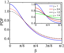
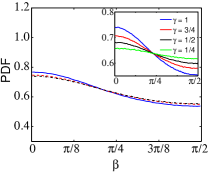
Figure 3: (Color online) PDFs of the angle $\beta$ between $\bm{p}$ and $\bm{e}_{1}$ for $\gamma=1$ and different $\mathit{Re}_{\lambda}$ in case (A) (left) and in case (B) (right). The insets show the PDF of $\beta$ for different values of $\gamma$ for runs A3 (left) and B3 (right). The color code is the same as in Fig. 2.

We have calculated the conditional PDFs of the alignment of particles conditioned on the sign of the Okubo–Weiss parameter OW ; PRMP11 , which distinguishes between vortical and extensional regions of the flow; the conditional PDFs do not deviate from their unconditional counterparts SM .

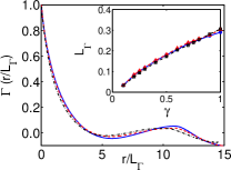
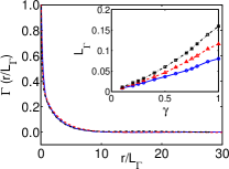
Figure 4: (Color online) Single-time two-point correlation function of $M$ as a function of the space separation rescaled by the correlation length. Left: run A1 (solid, blue curve), run A2 (dashed, red curve), run A3 (dot-dashed, black curve) for $\gamma=1$. Right: run B1 (solid, blue curve), run B2 (dashed, red curve), run B3 (dot-dashed, black curve) for $\gamma=1$. The insets show the correlation length as a function of $\gamma$; the color code is the same as in the main plots.

To quantify the spatial distribution of particle orientations, we define the correlation function $\Gamma(r)=[\langle M(\bm{r},t)M(\bm{0},t)\rangle-\langle M(\bm{r},t)\rangle\langle M(\bm{0},t)\rangle]/\langle M^{2}\rangle$, where $M(\bm{r},t)\equiv(2\cos^{2}\theta(\bm{r},t)-1)$ is the local nematic order parameter in 2D CL95 and $\langle\cdot\rangle$ denotes an average over time and over the tracer particles. The function $\Gamma(r)$ is shown in Fig. 4 for different values of $Re_{\lambda}$. In both the cases (A) and (B), the shape of $\Gamma(r)$ depends only weakly on $\mathit{Re}_{\lambda}$. However, in case (A), the order parameter of rods is correlated up to distances of the order of $5\%$ $L$ and is anti-correlated at large $r$; in case (B), $\Gamma(r)$ decays exponentially to zero. These behaviors are in accordance with the spatial distributions of orientations shown in Fig. 1. Furthermore, in case (A), the correlation length $L_{\Gamma}=[\int_{0}^{\pi}\Gamma(r)dr]/\Gamma(0)$ depends weakly on $\mathit{Re}_{\lambda}$, because the value of $L_{\Gamma}$ is determined principally by $k_{\mathrm{inj}}$; in case (B), the size of large-scale flow structures increases with increasing $\mathit{Re}_{\lambda}$ BM10 ; hence, $L_{\Gamma}$ increases accordingly. In both cases, $L_{\Gamma}$ is obviously an increasing function of $\gamma$.

Let us now examine the temporal autocorrelation function of $\bm{p}$. Both in cases (A) and (B), $C(t)=\langle\bm{p}(t)\cdot\bm{p}(0)\rangle$ decays exponentially to zero (Fig. 5), but the correlation time $\tau_{c}=\int_{0}^{\infty}C(t)dt$ is much shorter in the former case. The ratio $\tau_{c}/\tau_{\eta}$ increases as a function of both $Re_{\lambda}$ and $\gamma$; this behavior is similar to that observed in 3D turbulence, where the orientational dynamics of spheres decorrelates faster than that of rods pumir11 .

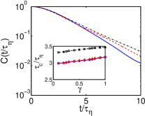
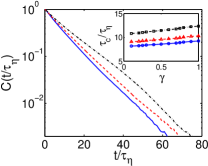
Figure 5: (Color online) Autocorrelation function of $\bm{p}$ as a function of the time separation rescaled by $\tau_{\eta}$ for different $\mathit{Re}_{\lambda}$ in case (A) (left) and in case (B) (right). The insets show the correlation time rescaled by $\tau_{\eta}$ as a function of $\gamma$ for different $\mathit{Re}_{\lambda}$. The color codes are the same as in Fig. 4.

Figure 6 shows the PDFs of the rotation rate $\dot{\theta}$ of particles for different values of $\mathit{Re}_{\lambda}$ (for the analogous PDFs at fixed $\mathit{Re}_{\lambda}$ and different $\gamma$, see SM ). Very large fluctuations characterize the statistics of $\dot{\theta}$, as has been observed in 3D turbulence toschi12 . However, the probability of large fluctuations increases with increasing $\gamma$ and $\mathit{Re}_{\lambda}$ in case (A), whereas it depends weakly on $\gamma$ and $\mathit{Re}_{\lambda}$ in case (B). The main difference between 2D and 3D is the dependence of the mean-squared-rotation rate $\langle\dot{\theta}^{2}\rangle$ upon $\gamma$. In 3D, $\langle\dot{\theta}^{2}\rangle$ decreases as $\gamma$ increases and is thus smaller for rods than for spheres toschi12 . The reason for this behavior is that the tendency to align with $\bm{\omega}$ is stronger for elongated particles pumir11 ; toschi12 than for spheres. In 2D, such an alignment cannot take place and $\langle\dot{\theta}^{2}\rangle$ increases as $\gamma$ increases.

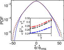
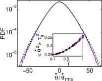
Figure 6: (Color online) PDFs of $\dot{\theta}$ rescaled by $\dot{\theta}_{\mathrm{rms}}=\sqrt{\langle\dot{\theta}^{2}\rangle}$ for $\gamma=1$ and different $\mathit{Re}_{\lambda}$ in case (A) (left) and in case (B) (right). The insets show the mean-square rotation rate multiplied by $\tau_{\eta}^{2}$ as a function of $\gamma$. The color codes are the same as in Fig. 4.

We have examined the statistics of the orientational and rotational dynamics of elliptical tracers in 2D, homogeneous and isotropic turbulence. By considering two sets of simulations with different $k_{\mathrm{inj}}$, we have shown that these properties depend on the scale at which the turbulent flow is generated. In the small-$k_{\mathrm{inj}}$ case, the spatial correlation of the nematic order parameter indicates the existence of large-scale structures in the spatial distribution of $\bm{p}$, which are absent in the intermediate-$k_{\mathrm{inj}}$ case. Moreover, the probability of $\bm{p}$ being aligned with $\nabla\times\bm{\omega}$ or $\bm{e}_{1}$ is much lower for intermediate $k_{\mathrm{inj}}$ than for small $k_{\mathrm{inj}}$. These differences can be explained by noting that the dynamics of fluid particles is different in the direct- and inverse-cascade regimes BC00 ; BS02 , and hence the Lagrangian statistics of $\nabla\bm{u}$ depends on $k_{\mathrm{inj}}$ (see, e.g., $\tau_{S_{11}}$, $\tau_{S_{12}}$, and $\tau_{\omega}$ given in Table 1, as well as the Lagrangian autocorrelation functions of the components of $\nabla\bm{u}$ reported in SM ). Our study sheds new light on the qualitative differences between 2D and 3D homogeneous, isotropic fluid turbulence. These differences lead to a weaker alignment between $\bm{p}$ and $\nabla\times\bm{\omega}$ in 2D as compared to the alignment between $\bm{p}$ and $\bm{\omega}$ in 3D and to a different dependence of $\langle\dot{\theta}^{2}\rangle$ upon $\gamma$ (as $\gamma$ increases, $\langle\dot{\theta}^{2}\rangle$ increases in 2D but decreases in 3D). We hope our comprehensive study of the statistical properties of elliptical tracer particles in 2D, homogeneous and isotropic turbulent fluid flows will stimulate experimental studies of such particles.

- (1) A.S. Monin and A.M. Yaglom, Statistical Fluid Mechanics (Dover Publications, Inc., Mineola, NY, 1975).
- (2) U. Frisch, Turbulence: The Legacy of A.N. Kolmogorov (Cambridge University Press, Cambridge, England, 1995).
- (3) T. Bohr, M.H. Jensen, G. Paladin, and A. Vulpiani, Dynamical Systems Approach to Turbulence (Cambridge University Press, Cambridge, England, 1998)
- (4) R. Pandit, P. Perlekar, and S.S. Ray, Pramana - Journal of Physics 73, 157 (2009).
- (5) G. Falkovich, K. Gawȩdzki, and M. Vergassola, Rev. Mod. Phys. 73, 913 (2001).
- (6) F. Toschi and E. Bodenschatz, Annu. Rev. Fluid Mech. 41, 375 (2009).
- (7) J.P.L.C. Salazar and L.R. Collins, Annu. Rev. Fluid Mech. 41, 405 (2009).
- (8) D.L. Koch and G. Subramanian, Annu. Rev. Fluid Mech. 43, 637 (2011).
- (9) J.P. Chen and D. Lamb, J. Atmos. Sci. 51, 1206 (1994).
- (10) F. Lundell, L.D. Söderberg, and P.H. Alfredsson, Annu. Rev. Fluid Mech. 43, 195 (2011).
- (11) E.S.G. Shin and D.L. Koch, J. Fluid Mech. 540, 143 (2005).
- (12) A. Pumir and M. Wilkinson, New J. Phys. 13 093030 (2011).
- (13) S. Parsa, E. Calzavarini, F. Toschi, and G. A. Voth, Phys. Rev. Lett. 109, 134501 (2012).
- (14) M. Wilkinson and H.R. Kennard, J. Phys. A: Math. Theor. 45, 455502 (2012).
- (15) D. Vincenzi, J. Fluid Mech. 719, 465 (2013).
- (16) L. Chevillard and C. Meneveau, J. Fluid Mech. 737, 571 (2013).
- (17) K. Gustavsson, J. Einarsson, and B. Mehlig, Phys. Rev. Lett. 112, 014501 (2014).
- (18) S. Parsa, J.S. Guasto, M. Kishore, N.T. Ouellette, J.P. Gollub, and G.A. Voth, Phys. Fluids 23, 043302 (2011).
- (19) M. Wilkinson, V. Bezuglyy, and B. Mehlig, Phys. Fluids 21, 043304 (2009); V. Bezuglyy, B. Mehlig, and M. Wilkinson, Europhys. Lett. 89, 34003 (2010)
- (20) M. Lesieur, Turbulence in Fluids (Springer, Dordrecht, The Netherlands, 2008).
- (21) G. Boffetta and R.E. Ecke, Annu. Rev. Fluid Mech. 44, 427 (2012).
- (22) P. Perlekar and R. Pandit, New J. Phys. 12, 023033 (2010) and references therein.
- (23) G.B. Jeffery, Proc. R. Soc. Lond. A 102, 161 (1922).
- (24) C. Canuto, M. Y. Hussaini, A. Quarteroni, and T. A. Zang, Spectral Methods in Fluid Dynamics (Springer-Verlag, Berlin, 1988).
- (25) S. M. Cox and P. C. Matthews, J. Comput. Phys. 176, 430 (2002).
- (26) W. Press, B. Flannery, S. Teukolsky, and W. Vetterling, Numerical Recipes in Fortran (Cambridge University Press, Cambridge, 1992).
- (27) A. Okubo, Deep-Sea Res. Oceanogr. Abstr. 17, 445 (1970); J. Weiss, Physica (Amsterdam) 48D, 273 (1991).
- (28) P. Perlekar, S.S. Ray, D. Mitra, and R. Pandit, Phys. Rev. Lett. 106, 054501 (2011).
- (29) See Supplemental Material at URL for the spatiotemporal evolution of the plots shown in Fig. 1, the PDFs of the alignment conditioned on the sign of the Okubo–Weiss parameter, the PDFs of for different values of , and the Lagrangian statistics of .
- (30) P.M. Chaikin and T.C. Lubensky, Principles of Condensed Matter Physics (Cambridge University Press, Cambridge, England, 1995).
- (31) G. Boffetta and S. Musacchio, Phys. Rev. E 82, 016307 (2010).
- (32) G. Boffetta and A. Celani, Physica (Amsterdam) 280A, 1 (2000).
- (33) G. Boffetta and I.M. Sokolov, Phys. Fluids 14, 3224 (2002).