Testing Lambda and the Limits of Cosmography
with the Union2.1 Supernova Compilation

Abstract

We present a cosmographic study designed to test the simplest type of accelerating cosmology: a flat universe with matter and a cosmological constant ($\Lambda$). Hubble series expansions are fit to the SCP Union2.1 supernova data set to estimate the Hubble Constant ($H_{0}$), the deceleration parameter ($q_{0}$), and the jerk parameter ($j_{0}$). Flat $\Lambda$CDM models always require $j_{0}=1$, providing a single-parameter test of the entire paradigm. Because of convergence issues for $z\gtrsim 1$, we focus on expansions using the newer redshift variable $y$; and to estimate the effects of “model-building uncertainties” – the dependence of the output results upon the fitting function and parameters used – we perform fits using five different distance indicator functions, and four different polynomial orders. We find that one cannot yet use the supernova data to reliably obtain more than four cosmological parameters; and that cosmographic estimates of $j_{0}$ remain dominated by model-building uncertainties, in conjunction with statistical and other error sources. While $j_{0}=1$ remains consistent with Union2.1, the most restrictive bound that we can place is $j_{0}\sim[-7.6,8.5]$. To test the future prospects of cosmography with new standard candle data, ensembles of mock supernova data sets are created; and it is found that the best way to reduce model-building uncertainties on lower-order Hubble parameters (such as $\{H_{0},q_{0},j_{0}\}$) is by limiting the redshift range of the data. Thus more and better $z\lesssim 1$ data, not higher-redshift data, is needed to sharpen cosmographic tests of flat $\Lambda$CDM.

1 Introduction and Motivation

The discovery of the acceleration of the universe (Riess et al., 1998; Perlmutter et al., 1999a) solved certain major cosmological problems, such as the “Age Crisis,” while reconciling the low density of matter (as inferred from structure formation) with the fact of overall spatial flatness (Turner, 2002). As a consequence, however, it created a new, fundamental problem: the entirely unknown nature of the force, effect, or substance responsible for this observed cosmic acceleration.

Many different approaches have been taken toward explaining this (real or apparent) acceleration; and there is a voluminous literature on the different paradigms considered, which include modified gravity (see Clifton et al., 2012, for a review), inhomogeneity-perturbed observational effects (e.g., Kantowski, 1969, 1998; Celériér & Schneider, 1998; Tomita, 2001; Alnes et al., 2006; Chung & Romano, 2006; Garfinkle, 2006; Biswas & Notari, 2008; Bolejko, 2008), and structure-formation-induced “backreaction” (e.g., Saulder et al., 2012; Bochner, 2013, and references therein). In general, however, the standard approach usually involves the introduction of “dark energy” (Perlmutter et al., 1999b), a hypothesized substance which possesses negative pressure to drive the acceleration, yet which must remain largely unclumped in order to avoid a conflict with structure formation models. But whether or not a distinct dark energy substance turns out to be the correct culprit, determining the true nature of this mysterious effect represents an exceptionally difficult observational challenge.

The question of whether or not dark energy exists in the form of a cosmological constant ($\Lambda$) is an extremely consequential one. The predominance of $\Lambda$ in the universe would lead to two well-known fine-tuning problems: one being the “Cosmological Constant Problem” (Kolb & Turner, 1990), relating to its magnitude being nonzero but far below the Planck (or any ‘natural’) scale; and the other being the “Coincidence Problem” (e.g., Arkani-Hamed et al., 2000), the question of why $\Omega_{\Lambda}\sim O[1]\cdot\Omega_{M}$ in the current epoch (just in time to be seen by observers like ourselves), rather than being unmeasurably small or fatally large. Furthermore, a study of virialization with dark energy (Maor & Lahav, 2005) shows that $\Lambda$ is not even on the continuum of perfect fluids with general $w(z)$, but instead is a uniquely distinct entity. Thus the case for (or against) $\Lambda$ is a question with far-reaching implications.

To determine the physical nature of the dark energy – i.e., its equation of state (EoS), $w(z)\equiv P/\rho$ – one must place constraints up to (at least) the third-order term in the luminosity distance series expansions, since the first two terms tell us only about the present-day expansion rate (the Hubble Constant, $H_{0}$), and the effective amount of dark energy acting now ($q_{0}\sim w^{\mathrm{DE}}_{z=0}\cdot\Omega_{\mathrm{DE}}$). Measuring its detailed, time-evolving behavior requires information beyond those first two terms, and so is very difficult to estimate. The issue of determining how many accurately estimated parameters can be obtained from cosmological data sets – and how best to obtain them – has been the subject of detailed analyses (e.g., Linder & Huterer, 2005; Ruiz et al., 2012), which generally highlight the difficulty of measuring $w(z)$.

It is a common practice (e.g., Suzuki et al., 2012) to combine a variety of different, complementary data sets – such as compilations of Type Ia Supernovae (SNe), Cosmic Microwave Background (CMB) maps, standard ruler measurements from Baryon Acoustic Oscillations, and so on – to obtain constraints on $w(z)$. But of all the different types of cosmological data sets, SN Ia standard candles are the only data which directly and continuously trace out the cosmic expansion as it evolved in the ‘recent’ (moderate-redshift) universe, as the cosmic acceleration “took over”; as a consequence, though beset by systematics (Ruiz et al., 2012) and large scatter, they are clearly the data most naturally suited for evaluating the cosmologically recent onset of acceleration, and for detailing its precise time evolution. Furthermore, in the 9-Year WMAP CMB data release, it was specifically the supernova data set which dramatically drove the combined analysis toward the $\Lambda$ condition of $w(z)\simeq w_{0}\simeq-1$ (see Figure 10 of Hinshaw et al., 2013); and from the Planck 2013 CMB results, it is similarly clear (from their comparisons of different SNe compilations) that the preferred parameter space for the dark energy EoS is particularly sensitive (see Figure 36 of Ade et al., 2014) to the choice of SNe data set used. It is therefore crucial that we properly interpret the ‘story’ being told by the best available SNe data; and so, one goal of this paper is to illustrate what the most critically relevant data set – SN Ia standard candles – can and cannot yet prove about the cosmological constant. In particular, we focus here upon the comprehensive and homogeneously analyzed supernova data set known as the SCP Union2.1 SNe compilation (Suzuki et al., 2012).

Now, if one’s primary question is to determine, “What kind of dark energy is accelerating the universe?,” then the natural approach would be to evaluate time-varying EoS models for $w(z)$ by adopting some preferred parameterization – such as “CPL” (Chevallier & Polarski, 2001; Linder, 2003), $w(z)=w_{0}+w_{a}[z/(1+z)]$ – and fitting those parameters ($w_{0},w_{a}$) to the SNe data. But though commonly employed, this method has certain disadvantages.

First, the negative-pressure properties of dark energy (DE) imply that its density (and cosmological influence) were significantly lower at high redshift, making $w(z)$ an increasingly limp probe of the evolution of the acceleration as $z$ increases. Second, specifically testing the cosmological constant requires one to constrain the two-dimensional phase space of $(w_{0},w_{a})$, to simultaneously verify two conditions for $\Lambda$, $w_{0}=-1$ and $w_{a}=0$; but given the limited information content of the data, a one-parameter test may be preferable, which can be done via the “jerk parameter,” $j_{0}$, related to the third derivative of the scale factor $a(t)$. Lastly, the most fundamental information being sought is not necessarily about what the dark energy (if it exists) is doing, but about what the Universe is doing. As noted in Riess et al. (2007), the assumption of “a simple dark-energy parameterization [like CPL] is equivalent [their emphasis] to a strong and unjustified prior on the nature of dark energy.” Therefore, in the interest of placing all of the alternative paradigms (DE, backreaction, local voids, etc.) on an equal footing, rather than assuming any DE EoS function $w(z)$ at all, we instead use the kinematic approach known as “cosmography” (e.g., Cattoën & Visser, 2007a, b, 2008), to directly extract the Hubble series from the data without employing any prior assumptions about the physics underlying the cosmic expansion history.

In the cosmographic method, one expands the luminosity distance (and/or related distance scale functions) in Taylor series using some choice of redshift parameter. The first three series terms introduce, respectfully: the Hubble Constant, $H_{0}\equiv\dot{a}_{0}/a_{0}$; the deceleration parameter, $q_{0}\equiv-(\ddot{a}_{0}/a_{0})H_{0}^{-2}$ (which can be translated into the effective amount of “dark energy,” if desired); and the jerk parameter, $j_{0}\equiv(\dot{\ddot{a}}_{0}/a_{0})H_{0}^{-3}$ (which can be translated into information about the evolution of the dark energy EoS – e.g., $w_{a}$ – if desired). A key advantage for cosmography in testing the hypothesis of a spatially flat universe containing only matter and $\Lambda$, is that such models must have $j(z)\equiv j_{0}=1$ for all time (Dunajski & Gibbons, 2008) – regardless of the relative amounts of $\Omega_{\Lambda}$ and $\Omega_{M}$ – as long as $\Omega_{\Lambda}+\Omega_{M}=1$. Thus the entire hypothesis of flat $\Lambda$CDM can be falsified simply by searching for any deviation from $j_{0}=1$. Thus $q_{0}$ (like $H_{0}$) becomes a “nuisance parameter” in this context, and the problem is indeed reduced to a search through a one-dimensional parameter space.

Cosmographic testing of $j_{0}$ via SNe data fitting has been done before, though with frustratingly discordant results. Several recent tests have used the SCP Union2 (Amanullah et al., 2010) supernova compilation (consisting of 557 SNe passing all data cuts, 23 fewer than Union2.1), in combination with different selections of auxiliary data sets being chosen for different analyses. For example, Xu & Wang (2011) used Union2 SNe data (plus GRB and observational $H(z)$ data, etc.) to obtain a $\Lambda$-consistent (but fairly weak) constraint of approximately $j_{0}\simeq-5\pm 7$. Similarly, Cai & Tuo (2011) obtained SNe-only estimates (using two different redshift expansions) of $j_{0}\simeq-1.83^{+5.85}_{-4.79}$ and $j_{0}\simeq-6.56^{+11.12}_{-21.40}$. Xia et al. (2012) used different data set combinations (all in conjunction with Union2 SNe) for fitting luminosity distance curves, to obtain a variety of results from $j_{0}\simeq-7$ all the way to $j_{0}\simeq 5$, with the $\Lambda$-required result of $j_{0}\equiv 1$ being within the uncertainties for some of the fitted data combinations, but lying far outside the error bars for others. Demianski et al. (2012) found low $j_{0}$ values, including results more than 2$\sigma$ away from unity (though within 3$\sigma$), with variations of approximately $j_{0}\simeq 0.1-0.9$ for their different fits. This tendency of extreme variability of the $j_{0}$ results for different fitting functions, expansion variables, and/or data sets has typically been a hallmark of these and other cosmographic studies (e.g., Capozziello et al., 2012; Aviles et al., 2012) done with this (and prior) SNe data compilations.

The important point to take away from these discrepant results, is not that one must strive to find the “right” fitting function, variables, or data sets – but that there is no absolutely “right” set of parameters. Instead, we must understand why different cosmographic fitting models give such differing results. The essential difficulty was explained and quantified (though with older SNe data) in a landmark study by Cattoën & Visser (2007a, b, 2008), in which they showed how the variability of parameter estimates is due to Hubble series truncation, because of the small number of terms that could be reliably estimated from the data: fewer fitting parameters leads to greater “model-building uncertainty” (referring to the variability of the output results, when different fitting models are used); but more fitting parameters (e.g., $H_{0}$, $q_{0}$, $j_{0}$, $s_{0}$, $c_{0},\dots$) leads to greater statistical uncertainty in the best-fit values of each term (thus leading to unphysical parameter estimates, consistent statistically only because of their huge error bars). Our results in this research verify that intuition. Thus one cannot do better than to find the ‘sweet spot’ which balances the model-building uncertainties on $H_{0}$, $q_{0}$, $j_{0},\dots$ due to series truncation (by not using too few best-fit model parameters), versus limiting the statistical uncertainties on those parameters (by not using too many parameters), given the limited statistical power of the SNe data in hand.

While such “model-building” uncertainties have been viewed somewhat mysteriously (e.g., Aviles et al., 2012), their origin is simply due to the limitation of having to fit a complicated (measured flux) curve with a Taylor series that has too few terms. For example, consider trying to fit a parabola of data (i.e., $y=az+bz^{2}$) with a linear theory (i.e., $y=mz$). There is no uniquely correct way of doing this; and by variously emphasizing either the low-$z$ or high-$z$ data (e.g., via multiplication by various powers of $(1+z)$), one will get different ‘best-fit’ slopes $m$. To fix this problem, there are two straightforward ways of getting a uniquely determined answer: either add more polynomial terms to the Taylor expansion fit (i.e., $y=m_{1}z+m_{2}z^{2}+\dots$), or cut off the data to leave only a small range in $z$, so that the ‘curve’ of the parabola does not manifest itself. Unfortunately, as our results prove, though increasing the number of best-fit Taylor series coefficients from 3 (the minimum needed for estimating $j_{0}$) to 6 does indeed reduce the model-building uncertainties to very small levels, the act of including more fitting terms $m_{i}$ also does lead to a dramatic increase in the statistical uncertainties on all of the best-fit coefficients, including the lower-order ones actually used to calculate $H_{0}$, $q_{0}$, and $j_{0}$. Similarly, cutting off the SNe data above some high-$z$ threshold also increases the statistical uncertainties, despite successfully reducing the model-building uncertainties. Thus all that one can strive for, is to find a balance between the statistical versus the model-building uncertainties, in order to determine what is “the best that one can do” in a cosmographic analysis of a given data set.

This problem of parameter fitting indeterminacy is not unique to cosmographic methods, but also occurs with fits using dark energy EoS functions with a very limited number of best-fit coefficients – as demonstrated, for example, in Riess et al. (2007), and also by the “Mirage of $w=-1$” problem (Linder, 2007) for fits with $w(z)$ models limited to a single, constant value (i.e., $w(z)\equiv w_{0}$). No type of theoretical model is immune to model-building uncertainties, if the number of adjustable parameters used in the fitting process is insufficient to model the curve followed by the data.

The core of the aforementioned study (Cattoën & Visser, 2007a, b, 2008) involved a comprehensive collection of fits using five different distance indicator functions: the traditional luminosity distance $d_{\mathrm{L}}(z)$, along with four other functions related to $d_{\mathrm{L}}$ by different powers of ($1+z$). And considering series convergence issues for $z\gtrsim 1$, they also fit the data to series expansions in “$y$-redshift” variable, $y\equiv z/(1+z)$. Our work here builds upon and expands their work, utilizing newer SNe data and higher-order polynomial fitting functions. To that end, we have conducted a systematically designed study of the SCP Union2.1 data set (a compilation of 580 SNe Ia passing all data cuts), with a full set of best-fit functions that includes: (i) five different distance indicator functions; (ii) expansions done using both $z$-redshift and $y$-redshift; and, (iii) Hubble series fits using several different polynomial orders (with functions possessing $3$, $4$, $5$, and $6$ fitted parameters, respectively). A fully comprehensive discussion of all of these simulations and their implications is available in a separate preprint (Bochner et al., 2014), henceforth BPDv2; here we provide an overview of our methodology, and a discussion of the key results.

From our overall set of $5\times 2\times 4=40$ fits to the Union2.1 compilation, it is clear that the value of the jerk parameter $j_{0}$ cannot yet be narrowed down with great precision, even using Union2.1 as a virtually continuous tracer over most of the acceleration epoch. A useful quote of our constraints (see Section 3) results in a range for the jerk parameter of $j_{0}\sim[-7.6,8.5]$ – which, though being completely consistent with a cosmological constant ($j_{0}\equiv 1$), still remains far from providing a stringent test of $\Lambda$ versus the more dynamical forms of dark energy. Finally, two classes of mock data sets are constructed (involving 200 randomized simulations for each case), which are evaluated to determine how the current constraints may be improved with future supernova data.

2 Cosmographic Methodology

Due to the expansion of the universe, the definition of distance in cosmology (between an early emitter and a later observer) is fundamentally ambiguous. For example, the “luminosity distance” $d_{\mathrm{L}}(z)$ is typically defined from the relationship between the known luminosity $L$ for a standard candle (e.g., a SN Ia), and its measured flux $F$, via: $F=L/(4\pi d_{\mathrm{L}}^{2})$. In FLRW models, this definition sets $d_{\mathrm{L}}\equiv a_{0}r(1+z)$, where $a_{0}$ is the present-day scale factor and $r\equiv r(z)$ is the comoving coordinate distance to the emitting object. Alternatively, the “angular diameter distance” $d_{\mathrm{A}}(z)$ is typically defined from the relationship between the measured angular size $\theta$ of a “standard ruler,” and its known physical diameter $D$, as: $\theta=D/d_{\mathrm{A}}$. This definition sets $d_{\mathrm{A}}\equiv a_{0}r/(1+z)$, and hence, $d_{\mathrm{A}}=d_{\mathrm{L}}(1+z)^{-2}$. There is, however, no end to the different types of distance indicator functions which one may introduce; for example (see Cattoën & Visser, 2007a), one could also consider the “photon flux distance,” $d_{\mathrm{F}}=d_{\mathrm{L}}(1+z)^{-1/2}$; the “photon count distance,” $d_{\mathrm{P}}=d_{\mathrm{L}}(1+z)^{-1}$; the “deceleration distance,” $d_{\mathrm{Q}}=d_{\mathrm{L}}(1+z)^{-3/2}$; and/or any other distance indicator function related by various powers or functions of $(1+z)$.

Despite their evocative names (and idiosyncratic origins), all of these distance scale functions are equally good expressions to use for fitting to any type of cosmological data set. Other than traditional usage, there is no particular reason why one must (or should) fit flux data to the “luminosity distance” function, $d_{\mathrm{L}}\propto F^{-1/2}$, as opposed to any other function of flux $F$ (and redshift $z$). The key realization by Cattoën & Visser (2007a, b, 2008), was that the use of a different distance function to fit the same data ends up yielding radically different results. In particular, the best-fit value of a particular cosmological parameter will be changed, from one distance scale function to the next, in an evenly spaced manner (which they explained theoretically as an effect of series truncation, resulting from the unavoidably finite number of best-fit series coefficients). This same behavior is also seen in our results here, and so the error budget to be minimized must include these model-building uncertainties, in tandem with the statistical uncertainties on the estimated cosmological parameters.

Complete expressions for each Hubble series for $\{d_{\mathrm{L}}(z),d_{\mathrm{F}}(z),d_{\mathrm{P}}(z),d_{\mathrm{Q}}(z),d_{\mathrm{A}}(z)\}$, and for $\{d_{\mathrm{L}}(y),\dots,d_{\mathrm{A}}(y)\}$ – up to three polynomial terms, the minimum number required to estimate $j_{0}$ – have been given in Cattoën & Visser (2007a, and their many related references). Furthermore, series expressions are also are given for these functions in the alternative form, $\ln\{[d_{\mathrm{L}}(z)]/z\}$, etc., which conveniently removes a varying but cosmologically irrelevant term from the plotted and fitted functions. Due to this and other advantages, we have performed fits (BPDv2) using their ten different series expansions for: $\ln\{[d_{\mathrm{L}}(z)]/z\},\dots,\ln\{[d_{\mathrm{A}}(z)]/z\}$, and: $\ln\{[d_{\mathrm{L}}(y)]/y\},\dots,\ln\{[d_{\mathrm{A}}(y)]/y\}$. Due to the unavoidable series convergence concerns for $z$-redshift, however, in this paper we focus exclusively on the fits performed using the $y$-redshift variable.

As one example case to describe explicitly, consider the expansion:

$$\ln\{[d_{\mathrm{P}}(y)]/y\} = \ln(\frac{c}{H_{0}})+\frac{1}{2}(1-q_{0})y$$ (1)

$$+ \frac{1}{24}(5-2q_{0}+9q_{0}^{2}-4j_{0})y^{2}+O[y^{3}],$$

where we have already assumed flatness everywhere (i.e., setting terms like $(j_{0}+\Omega_{0})$ equal to $(j_{0}+1)$ in all expressions).

The Union2.1 compilation data is described in Suzuki et al. (2012), and the data itself is publicly available from the Supernova Cosmology Project website, http://supernova.lbl.gov/Union. Their “Magnitude vs. Redshift Table” lists $(z,\mu,\sigma_{\mu})$ for each SN Ia, where $\mu$ represents the “distance modulus” data, and the $\sigma_{\mu}$ are their (uncorrelated) statistical errors. The $z$-redshift values can be converted into $y$-redshift as discussed above, and each of the $(\mu,\sigma_{\mu})$ values can be trivially converted into data and uncertainty values in any form required – e.g., $\ln(d_{\mathrm{P}}/y)$ – for comparison to expansions such as Equation 1.

Now consider a fitting polynomial of the form:

$$F(y)\equiv p_{0}+p_{1}y+p_{2}y^{2}+\cdots+p_{n}y^{n}~{}.$$ (2)

This function, going up to order $y^{n}$, will possess $N\equiv(n+1)$ optimizable parameters. We need to use at least $N=3$ polynomial terms in order to estimate $j_{0}$, though in principle one can include any number of additional high-order series terms. Though the formulas for $\{H_{0},q_{0},j_{0}\}$ – derived from the first three terms of expressions like Equation 1 – do not change based on $N$, we will see that their best-fit values do in fact depend significantly upon $N$, due to changing statistical and model-building uncertainties. Our modeling includes the results from fits using $N=\{3,4,5,6\}$ (for each redshift variable and distance scale function), evaluating each fit in light of the $F$-test of additional terms (Cattoën & Visser, 2007a, b, 2008).

When fit to a SNe data set with a total of $N_{\textrm{SN}}$ supernovae (where $N_{\textrm{SN}}=580$ for Union2.1), a polynomial $F(y)$ with $N$ terms will result in a best-fit with $(N_{\textrm{SN}}-N)$ degrees of freedom. We then compute:

$$\chi^{2}(p_{0},p_{1},\dots,p_{n})=\sum^{580}_{i}\frac{[d_{i}-F(y_{i})]^{2}}{\sigma_{i}^{2}}~{},$$ (3)

where $(d_{i},\sigma_{i})$ are the data point and statistical uncertainty for the $i^{\mathrm{th}}$ supernova. This $\chi^{2}$ is then minimized in order to determine the best-fit values and sigmas of $(p_{0},p_{1},\dots,p_{n})\equiv\vec{p}$, for this form of fitting function.

The optimization is done using standard statistical techniques. The elements of the coefficient matrix $\textbf{{A}}\equiv\{a_{jk}\}$ (and an auxiliary vector $\vec{b}\equiv\{b_{k}\}$) are calculated via:

$$a_{jk}=\sum^{580}_{i}\frac{(x_{i})^{j}(x_{i})^{k}}{\sigma_{i}^{2}}~{},~{}b_{k}=\sum^{580}_{i}\frac{(d_{i})(x_{i})^{k}}{\sigma_{i}^{2}}~{},$$ (4)

where $x_{i}$ is the $i^{\mathrm{th}}$ redshift value (either $z_{i}$ or $y_{i}$), and $(j,k)$ run through $\{0,n\}$. Then with the parameter error covariance matrix $\textbf{{Z}}\equiv\{z_{jk}\}=\textbf{{A}}^{-1}$, we get the optimized parameters as $\vec{p}=\textbf{{Z}}\vec{b}$, with their sigmas obtained from the diagonal elements of Z (i.e., $\sigma_{p_{k}}=\sqrt{z_{kk}}$).

Once these best-fit polynomial coefficients have been determined, we can invert the appropriate Hubble series to obtain the optimized cosmological parameters corresponding to them. In cosmographic expansions like Equation 1 for the various distance scale functions, each new series term introduces one new cosmological parameter; and our results show that the uncertainties typically get significantly larger for each higher-order coefficient (i.e., $\sigma_{p_{0}}\ll\sigma_{p_{1}}\ll\sigma_{p_{2}}\ll\sigma_{p_{3}}\dots$, is usually true). It is therefore a good procedure to obtain $H_{0}$ (and $\sigma_{H_{0}}$) solely from $p_{0}$ (in fact, the Hubble constant only appears in $p_{0}$), and to get $q_{0}$ solely from $p_{1}$; we also get $j_{0}$ solely from $p_{2}$ (regardless of the total number of expansion terms, $N\geq 3$), though with some dependence on $q_{0}$ (and thus $p_{1}$).

For the example discussed here ($\ln\{[d_{\mathrm{P}}(y)]/y\}$), we compare Equations 1 and 2 to obtain:

$$H_{0}=ce^{-p_{0}}~{},$$ (5)

$$q_{0}=1-2p_{1}~{},$$ (6)

$$j_{0}=-6p_{2}+\frac{1}{4}(5-2q_{0}+9q_{0}^{2})~{}.$$ (7)

Additionally, from the Friedmann Robertson-Walker acceleration equation, plus the definition of $q_{0}$, one obtains $q_{0}=(1+3w_{0})/2$, which can be inverted to give:

$$w_{0}=\frac{1}{3}(2q_{0}-1)~{}.$$ (8)

Note, though, that this EoS, $w_{0}\equiv w^{\mathrm{Obs}}_{0}$, does not represent the equation of state of any “dark energy” component by itself, but rather represents the effective total EoS of all of the cosmic contents averaged together, as inferred from observations of the overall evolution.

If one wishes, it is not difficult to relate these directly observed (i.e., cosmographic) parameters, $(w^{\mathrm{Obs}}_{0},j^{\mathrm{Obs}}_{0})$, to the EoS parameters of an underlying dark energy model with a dynamical equation of state $w^{\mathrm{DE}}(z)$, given some particular parameterization. Specifically, using the popular CPL parameterization, $w^{\mathrm{DE}}(z)=w^{\mathrm{DE}}_{0}+w^{\mathrm{DE}}_{\mathrm{a}}[z/(1+z)]=w^{\mathrm{DE}}_{0}+w^{\mathrm{DE}}_{\mathrm{a}}y\equiv w^{\mathrm{DE}}(y)$, along with the assumption of spatial flatness, one obtains (Bochner, 2011):

$$w^{\mathrm{Obs}}_{0}=\Omega_{\mathrm{DE}}~{}w^{\mathrm{DE}}_{0}~{},$$ (9)

which makes obvious sense; and:

$$j^{\mathrm{Obs}}_{0}=\{1+[\frac{9}{2}\Omega_{\mathrm{DE}}w^{\mathrm{DE}}_{0}(1+w^{\mathrm{DE}}_{0})]+[\frac{3}{2}\Omega_{\mathrm{DE}}w^{\mathrm{DE}}_{\mathrm{a}}]\}~{},$$ (10)

which gives $j^{\mathrm{Obs}}_{0}=1$ for the cosmological constant case (i.e., $w^{\mathrm{DE}}_{0}=-1,w^{\mathrm{DE}}_{\mathrm{a}}=0$), for any value of $\Omega_{\mathrm{DE}}$, just as required. But while these formulas allow one to convert our cosmographic parameter results into dark energy EoS parameters, we note again that since the two cosmographic parameters, $(w^{\mathrm{Obs}}_{0},j^{\mathrm{Obs}}_{0})$, are divided up (due to observational degeneracies) into three DE parameters, $(\Omega_{\mathrm{DE}},w^{\mathrm{DE}}_{0},w^{\mathrm{DE}}_{\mathrm{a}})$, one requires some auxiliary condition to be imposed among them in order to convert cosmographic constraints into dark energy constraints. We have therefore placed the translation of our Union2.1 cosmographic results into CPL parameter constraints in an appendix of BPDv2.

The parameter uncertainty values, $\{\sigma_{H_{0}},\sigma_{q_{0}},\sigma_{w_{0}}\}$, can be computed (using elementary error propagation) from, respectively, Equations 5,6, and 8 (and from similar equations for each of the various distance scale expansions). Since $H_{0}$ is drawn solely from $p_{0}$, and $\{q_{0},w_{0}\}$ are drawn solely from $p_{1}$, there are no issues of parameter covariance for them once the best-fit values of $\{p_{i}\}$ have been determined. But since $j_{0}$ depends upon both $p_{1}$ (via $q_{0}$) and $p_{2}$, the relevant terms in the parameter covariance matrix must be considered. For example (for $\ln\{[d_{\mathrm{P}}(y)]/y\}$), by re-writing Equation 7 as $j_{0}\equiv F(p_{1},p_{2})$, we obtain:

$$\sigma_{j_{0}}=\{[(\frac{\partial F}{\partial p_{1}})^{2}\cdot z_{11}]+[(\frac{\partial F}{\partial p_{2}})^{2}\cdot z_{22}]+[2(\frac{\partial F}{\partial p_{1}})(\frac{\partial F}{\partial p_{2}})\cdot z_{12}]\}^{1/2}~{},$$ (11)

with a similar $\sigma_{j_{0}}$ calculation being done for each different fitting function used.

Lastly, we note the obvious fact that the parameter estimation strategy outlined here is a considerably simplified version of the fitting process often used (e.g., Salzano et al., 2013) for obtaining state-of-the-art cosmological parameter constraints from SNe Ia. This is done deliberately, since more important (in this paper) than providing the most comprehensive possible constraints, is our goal of exploring the intricacies of the use of cosmography in standard candle data fitting, demonstrating its advantages and limitations independently of any particular survey or its systematics.

3 Cosmological Parameter Ranges Resulting from the Cosmographic Fits

First, examining the behavior of the cosmographic fits themselves, consider the example given in Figure 1, showing the SNe data in terms of photon count distance, $\ln(d_{\mathrm{P}}/y)$, plotted against its four relevant $y$-redshift polynomial fits. The residuals (not shown) for these different fits are very similar to one another – all fitting polynomials are very tightly constrained by the data below $z\lesssim 1.4$ – and despite a handful of individual SNe outliers (each possessing large error bars), no obvious systematic trends are apparent.

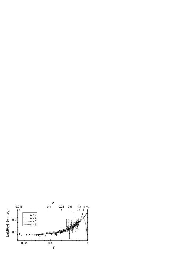
Figure 1: SN Ia data from the SCP Union2.1 compilation, binned and averaged (with $\Delta y=0.005$). The data is presented in the form $\ln(d_{\mathrm{P}}/y)$ and fit with four different polynomials $F(y)$ (as per Equation 2), with $N=\{3,4,5,6\}$ optimized polynomial coefficients, respectively. At the high-redshift end, the $N=5$ case runs away to larger (finite) values, while $N=6$ turns and drops downward; but the $N=3$ and $N=4$ fits change very slowly and remain close together as $y\rightarrow 1$, $z\rightarrow\infty$.

From Figure 1, it is clear that while all four fitting functions are virtually identical over the redshift range for which SNe data exists, the two higher-order polynomials ($N=5$ and $N=6$) become very poorly constrained as soon as the data runs out, for $y\gtrsim 0.59$ ($z\gtrsim 1.4$). This behavior foreshadows the results to be given below, that if one goes beyond the $N=4$ case, the best-fit cosmological parameter values start changing drastically. Conversely, since higher-order polynomial terms are needed in order to retain accuracy of the Taylor series far from $y=0$, the presence of higher-redshift data would actually require more series terms $N$ to be used in the cosmographic fitting process for the results to be reliable.

The output cosmological parameters derived (via Equations like 5-8) from our cosmographic polynomial fits to the Union2.1 data set are listed in Table 1 for the $y$-redshift expansions. These parameter estimation results are very much in line with our expectations from the prior studies by Cattoën & Visser (2007a, b, 2008). First, there is indeed a jump in each parameter value when going from one distance indicator function to the next, and the jumps are quite regularly spaced (within a given polynomial order $n$), just as expected. Furthermore, the variation in the results for different distance function fits is particularly large when fewer polynomial terms are used (i.e., smaller $N\equiv n+1$), making the effects of model-building error due to series truncation very obvious.

Table 1: Cosmographic Parameters from Hubble Series Expansions in $y$-Redshift, fitted to the SCP Union2.1 Type Ia supernova data set ($N_{\mathrm{SNe}}=580$).

Fitting Function	Fit Terms $N$	$H_{0}$	$q_{0}$	$w_{0}$	$j_{0}$
$\ln\{[d_{\mathrm{L}}(y)]/y\}$		69.722	-0.381	-0.587	-2.18 ($\pm 1.28$)
$\ln\{[d_{\mathrm{F}}(y)]/y\}$		69.879	-0.492	-0.661	-0.50 ($\pm 1.35$)
$\ln\{[d_{\mathrm{P}}(y)]/y\}$	3	70.036	-0.603	-0.735	1.24 ($\pm 1.43$)
$\ln\{[d_{\mathrm{Q}}(y)]/y\}$		70.194	-0.714	-0.809	3.04 ($\pm 1.50$)
$\ln\{[d_{\mathrm{A}}(y)]/y\}$		70.352	-0.825	-0.883	4.89 ($\pm 1.58$)
		($\pm 0.509-0.514$)	($\pm 0.154$)	($\pm 0.103$)	($\dots$)
$\ln\{[d_{\mathrm{L}}(y)]/y\}$		70.037	-0.623	-0.749	2.17 ($\pm 6.29$)
$\ln\{[d_{\mathrm{F}}(y)]/y\}$		70.003	-0.587	-0.725	1.22 ($\pm 6.23$)
$\ln\{[d_{\mathrm{P}}(y)]/y\}$	4	69.968	-0.551	-0.700	0.28 ($\pm 6.17$)
$\ln\{[d_{\mathrm{Q}}(y)]/y\}$		69.933	-0.514	-0.676	-0.65 ($\pm 6.11$)
$\ln\{[d_{\mathrm{A}}(y)]/y\}$		69.899	-0.478	-0.652	-1.58 ($\pm 6.05$)
		($\pm 0.668-0.669$)	($\pm 0.365$)	($\pm 0.243$)	($\dots$)
$\ln\{[d_{\mathrm{L}}(y)]/y\}$		69.374	0.115	-0.257	-17.89 ($\pm 18.16$)
$\ln\{[d_{\mathrm{F}}(y)]/y\}$		69.383	0.104	-0.264	-17.50 ($\pm 18.20$)
$\ln\{[d_{\mathrm{P}}(y)]/y\}$	5	69.391	0.092	-0.272	-17.11 ($\pm 18.24$)
$\ln\{[d_{\mathrm{Q}}(y)]/y\}$		69.399	0.081	-0.279	-16.71 ($\pm 18.28$)
$\ln\{[d_{\mathrm{A}}(y)]/y\}$		69.408	0.069	-0.287	-16.32 ($\pm 18.32$)
		($\pm 0.901-0.902$)	($\pm 0.775$)	($\pm 0.516$)	($\dots$)
$\ln\{[d_{\mathrm{L}}(y)]/y\}$		69.088	0.523	0.015	-32.64 ($\pm 47.18$)
$\ln\{[d_{\mathrm{F}}(y)]/y\}$		69.086	0.526	0.018	-32.80 ($\pm 47.16$)
$\ln\{[d_{\mathrm{P}}(y)]/y\}$	6	69.084	0.530	0.020	-32.95 ($\pm 47.14$)
$\ln\{[d_{\mathrm{Q}}(y)]/y\}$		69.082	0.533	0.022	-33.11 ($\pm 47.12$)
$\ln\{[d_{\mathrm{A}}(y)]/y\}$		69.080	0.537	0.024	-33.26 ($\pm 47.09$)
		($\pm 1.253-1.254$)	($\pm 1.471$)	($\pm 0.981$)	($\dots$)

For convenience in this discussion, we define the following terminology: let “$C^{N}_{\mathrm{X}}(R)$” represent the best-fit value of cosmological parameter “$C_{0}$” ($C\in\{H,q,w,j\}$), estimated with distance function $d_{\mathrm{``X^{\prime\prime}}}$ ($\mathrm{X}\in\{\mathrm{L},\mathrm{F},\mathrm{P},\mathrm{Q},\mathrm{A}\}$), when expanded in redshift variable “$R$” ($R\in\{z,y\}$), using $N$ terms in the polynomial expansion ($N\in\{3,4,5,6\}$). So for example, $H^{\mathrm{3}}_{\mathrm{L}}(y)=69.722$ is the best-fit value of $H_{0}$ from the $N=3$ SNe data fit done with $\ln\{[d_{\mathrm{L}}(y)]/y\}$. Relatedly, let “$\Delta_{\mathrm{LA}}C^{N}(R)$” represent the absolute net change in a cosmological parameter when going from the distance function at one “extreme” (given our admittedly arbitrary choice to use 5 distance indicator functions here), to the function at the other extreme: for example, $\Delta_{\mathrm{LA}}H^{3}(y)=|H^{3}_{\mathrm{L}}(y)-H^{3}_{\mathrm{A}}(y)|=|69.722-70.352|=0.63$.

From the numbers in Table 1, we see that the variation of the output parameters is crucially dependent upon the number of terms used in the fit. For example, $\Delta_{\mathrm{LA}}q^{3}(y)=0.444$, rendering the $N=3$ case almost useless for getting precision measurements of the strength of the acceleration (and thus of the DE EoS, $w_{0}$); while the $N=6$ case produces the dramatically more stable result of $\Delta_{\mathrm{LA}}q^{6}(z)=0.014$. And considering our interest in testing $\Lambda$ via precision measurements of $j_{0}$, we note that $\Delta_{\mathrm{LA}}j^{6}(y)=0.62$ (a reasonably small variation under the circumstances), but the $N=3$ case yields $\Delta_{\mathrm{LA}}j^{3}(y)=7.07$, which is not nearly small enough for precision tests of $\Lambda$.

We are therefore strongly motivated to go beyond the $N=3$ case, using as many optimizable parameters as possible. But how many terms can be usefully added? Despite the much smaller model-building uncertainty variations for the $N=6$ case – $\Delta_{\mathrm{LA}}w^{6}(y)=0.009$, as well as $\Delta_{\mathrm{LA}}j^{6}(y)=0.62$ – the actual best-fit cosmological parameter values from the $N>4$ cases make little physical sense. First, the values of $w^{5}_{\mathrm{X}}(y)$ and $w^{6}_{\mathrm{X}}(y)$ are all significantly greater than $(-1/3)$ – i.e., $\{q^{5}_{\mathrm{X}}(y),q^{6}_{\mathrm{X}}(y)\}>0$ – implying that the universe is not even accelerating according to the best-fit cosmic EoS from those fits. Furthermore, these cases also produce implausible best-fit estimates of the jerk parameter, with $j^{5}_{\mathrm{X}}(y)\sim-17$ to $-18$, and the $N=6$ case going as far away from $\Lambda$ as $j^{6}_{\mathrm{X}}(y)\sim-33$. Recalling Equation 10, and assuming $\Omega_{\mathrm{DE}}\sim 0.7$, a jerk parameter as negative as just $j_{0}\lesssim-4$ leads already to a DE evolution as strong as $w^{\mathrm{DE}}_{\mathrm{a}}\lesssim-4.8$ (for $w^{\mathrm{DE}}_{0}\sim-1$). Compare that result to those from Table 7 of Suzuki et al. (2012), which – over all of their cases, and including both statistical and systematic error ranges – gives a total estimated range of $w^{\mathrm{DE}}_{\mathrm{a}}\sim[-4.4,1.3]$. The best-fit parameters from our large-$N$ cosmographic fits are clearly very different from those quoted in such dynamical DE analyses.

It is important to note, however, that our large-$N$ cosmographic results here are not statistically inconsistent with those cited values. The reason for this, is that increasing the number of optimizable polynomial terms in the model fits, without any additional information content in the data to constrain them, results in greatly increased statistical uncertainties for each of the parameters. Our apparently unusual cosmological estimates are therefore due to those unavoidably large parameter uncertainties. In the fits just discussed, all of the $w^{5}_{\mathrm{X}}(y)$ and $w^{6}_{\mathrm{X}}(y)$ values are actually within 1$\sigma$ of $w^{\mathrm{Obs}}_{0}=-0.7$, considering their large error bars; and similarly, for $j^{5}_{\mathrm{X}}(y)$ and $j^{6}_{\mathrm{X}}(y)$, 8 out of the 10 cases are within 1$\sigma$ of the $j_{0}=1$ required by flat $\Lambda$CDM, with the other 2 cases not being far away. Thus these $N=\{5,6\}$ fits, while being statistically consistent with previous results, and demonstrably model-independent – i.e., effectively immune to model-building uncertainties (especially for $N=6$) – are limited to providing “reliable” but unimpressively broad cosmological constraints.

This cosmographic study therefore reveals the dilemma when using such data to attempt to estimate the jerk parameter to within $\Delta j_{0}\sim 1$ or so. If one sticks to $N=3$, then one may quote (for example) $j_{0}=j^{3}_{\mathrm{L}}(y)=-0.95\pm 0.14$ from the $\ln\{[d_{\mathrm{L}}(z)]/z\}$ fit, which seems like a fairly tight constraint that strongly excludes $\Lambda$CDM. But this result is completely spurious, since if one instead quoted the fit to $\ln\{[d_{\mathrm{A}}(z)]/z\}$, then the result would have the completely different value, $j_{0}=j^{3}_{\mathrm{A}}(y)=2.38\pm 0.24$. The mutual inconsistency of these numbers is due to the great sensitivity of the results to the fitting model chosen, when only three parameters are available for optimization. Thus model-building uncertainty completely trumps the statistical uncertainties quoted in such fits, and leads to a false confidence in the results for $j_{0}$. Going to $N=6$, on the other hand – which ensures the fitting-model-independence of the results (i.e., $\Delta_{\mathrm{LA}}j^{6}(y)<1$) – increases the statistical uncertainties on $j_{0}$ so much ($\sigma_{j_{0}}\sim 47$), that the constraints on flat $\Lambda$CDM from the cosmographic fit are very robust but extremely weak.

Note that this dilemma of having to balance precision versus accuracy is not due to the method of cosmography, per se – though cosmographic fitting does make the problem extremely transparent – but instead comes from the inherently limited information contained within the data set itself. Though one cannot draw an exact parallel between cosmography and the very different dynamical DE fits that start by assuming some EoS function $w(z)$, it is interesting to make some analogies. Our case with $N=3$ optimizable parameters, $\{H_{0},w_{0},j_{0}\}$ derived from $\{p_{0},p_{1},p_{2}\}$, is arguably analogous to constant-$w$ models, with the three optimizable parameters: $H_{0}$, $\Omega_{\mathrm{DE}}$, and $w\equiv w^{\mathrm{DE}}_{0}$. Given the unacceptable sensitivity that we have found here for the $N=3$ case to the particular fitting model chosen, in conjunction with the well-known “Mirage of $w=-1$” effect (Linder, 2007) for constant-$w$ models, we would suggest that constant-$w$ fitting models are not a reliable method for determining the properties of dark energy, and should not be used in cosmology at all, if possible. In addition, for cosmological analyses assuming any type of $w(z)$ functions, we would suggest that model-building uncertainties should always be explicitly estimated by fitting the same data with a variety of different DE models, to directly verify that the results do not change significantly when the design (or the number) of fitting parameters is altered.

Within the limitations discussed above, it remains interesting to estimate just how tight a constraint we can reasonably place upon $j_{0}$ (and thus $\Lambda$), with this data. Following Cattoën & Visser (2007a, b, 2008), the statistical justification of a particular fitting function can be put on a quantitative footing by considering the “$F$-test of additional terms” for each case. The improvement in going from a fit (to the 580 SNe data points) using $N$ fitting parameters – with chi-square value “$\chi^{2}_{N}$,” calculated via Equation 3 – to one with $(N+1)$ parameters (and chi-square $\chi^{2}_{N+1}$), is quantified by computing the statistic:

$$F_{\chi}=\frac{\chi^{2}_{N}-\chi^{2}_{N+1}}{\chi^{2}_{N+1}}\cdot[580-(N+1)]~{}.$$ (12)

Since this statistic follows an $F$-distribution with $\nu_{1}=1$ and $\nu_{2}=[580-(N+1)]$, we define the “$F$-test probability of improvement” (in going from $N$ to $(N+1)$ fitting terms), as:

$$F_{\mathrm{Prob.}}=[1-\int^{\infty}_{F_{\chi}}F\{x;1,[580-(N+1)]\}~{}dx]\times 100\%~{}.$$ (13)

For each of the fits described above, we calculated $\chi^{2}_{N}$ and used those values to compute $F_{\chi}$ (and thus $F_{\mathrm{Prob.}}$) in going from the next-lowest-$N$ case to that one; the resulting numbers are given in Table 2 for the $y$-redshift fits. (Note that these are the exact same fits whose cosmological parameters were given above, in Table 1, though here the fits are grouped together differently, to better demonstrate the effects of increasing $N$.)

Table 2: Fit Likelihoods for Expansions in $y$-Redshift, Union2.1 SNe data set.

Fitting Fcn.	Fit Terms $N$	$\chi^{2}$	$F_{\chi}$	$F_{\mathrm{Prob.}}$
	3	563.01	—	—
$\ln\{[d_{\mathrm{L}}(y)]/y\}$	4	562.47	0.549	54.1$\%$
	5	561.30	1.195	72.5$\%$
	6	561.20	0.109	25.8$\%$
	3	562.41	—	—
$\ln\{[d_{\mathrm{F}}(y)]/y\}$	4	562.33	0.084	22.8$\%$
	5	561.31	1.046	69.3$\%$
	6	561.20	0.117	26.7$\%$
	3	562.23	—	—
$\ln\{[d_{\mathrm{P}}(y)]/y\}$	4	562.20	0.026	12.8$\%$
	5	561.32	0.906	65.8$\%$
	6	561.20	0.125	27.6$\%$
	3	562.45	—	—
$\ln\{[d_{\mathrm{Q}}(y)]/y\}$	4	562.09	0.374	45.9$\%$
	5	561.33	0.776	62.1$\%$
	6	561.20	0.134	28.5$\%$
	3	563.08	—	—
$\ln\{[d_{\mathrm{A}}(y)]/y\}$	4	561.98	1.130	71.2$\%$
	5	561.34	0.657	58.2$\%$
	6	561.20	0.143	29.4$\%$

The lessons from this $F$-testing procedure are somewhat mixed. Table 2 only indicates a preference for $N=4$ over $N=3$ about half the time, even though the cosmological parameters for $N=4$ (e.g., $w^{4}_{\mathrm{X}}$ and $j^{4}_{\mathrm{X}}$ from Table 1) remain physically reasonable for all five distance functions. On the other hand, we have seen how the best-fit values of the $y$-redshift cosmological parameters start undergoing large changes already by $N=5$, yet the $F$-test results in Table 2 give opposite indications – that if one has already gone to $N=4$, then going to $N=5$ would be generally favored.

To sum up the best lessons that can be drawn from this variety of results: (i) The $N=5$ and $N=6$ fits are not useful for producing cosmological constraints here, due to very large statistical uncertainties, a result echoed (for the $N=6$ case) by poor performance in the $F$-tests; (ii) The estimated cosmological parameters from the $N=3$ fits are not generally reliable, due to large model-building uncertainties which lead to best-fit parameter variations (e.g., $\Delta_{\mathrm{LA}}w^{3}$, $\Delta_{\mathrm{LA}}j^{3}$) far in excess of their calculated statistical uncertainties; (iii) The $N=4$ fits are the best compromise for this SNe data set, moderating both the statistical and model-building uncertainties, while also being mildly preferred by the $F$-tests. (For comparison, note that the older SNe data considered in Cattoën & Visser (2007a, b, 2008) – the Riess Gold06 (Riess et al., 2004) and SNLS legacy05 (Astier et al., 2006) data sets – were not sufficient to go beyond even the $N=3$ case, which is the bare minimum number of parameters needed for estimating $j_{0}$ at all.)

To illustrate our cosmographic parameter results, the best-fit $j_{0}$ values for the $N=\{3,4\}$ $y$-redshift expansions are shown in Figure 2. The first conclusion evident from this plot, is that the $j_{0}=1$ line for flat $\Lambda$CDM is entirely consistent with these results, so that there is no statistically meaningful evidence of a departure from the cosmological constant. (Interestingly, the $N=3$ and $N=4$ trends for $j_{0}$ actually cross very close to that line, around $j_{0}\sim 0.6$.)

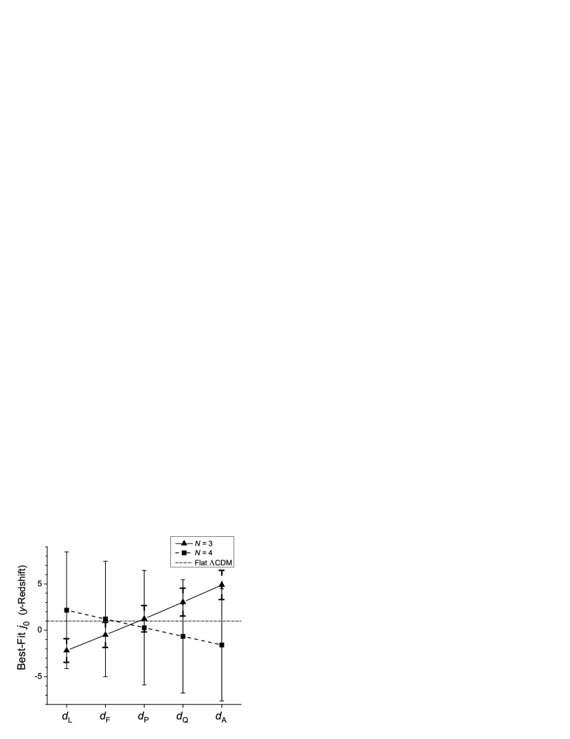
Figure 2: Values of Jerk Parameter $j_{0}$ from Union2.1 fits using distance functions $\ln\{[d_{\mathrm{X}}(y)]/y\}$ (with $\mathrm{X}\in\{\mathrm{L},\mathrm{F},\mathrm{P},\mathrm{Q},\mathrm{A}\}$), versus the number of series terms used, $N=\{3,4\}$.

From this figure (and from Table 1), we see that going from $N=3$ to $N=4$ cuts the model-building uncertainties nearly in half, from $\Delta_{\mathrm{LA}}j^{3}(y)=7.07$ to $\Delta_{\mathrm{LA}}j^{4}(y)=3.75$. The statistical uncertainties $\sigma_{j_{0}}$, however, are increased by a factor of about $\sim$$4-5$. The $N=3$ fits would seem actually to produce tighter constraints for $j_{0}$ than $N=4$ – except that it is readily apparent in Figure 2 that the $N=3$ trend of results has not “converged” in terms of model-building uncertainty, with the best-fit $j^{3}_{\mathrm{X}}(y)$ numbers changing from one distance-scale fitting function to the next by even more than each fit’s $\sigma_{j_{0}}$ value. Thus we must clearly take the $N=4$ case as our most reliable source of jerk parameter constraints.

Therefore, if we (somewhat informally) define the estimated range of $j_{0}$ as being bounded by its extreme values – folding together the (1$\sigma$) statistical uncertainties and model-building uncertainty – we get our “best possible” constraint from this cosmographic study: $\{j^{4}_{\mathrm{X}}(y)\pm\sigma_{j_{0,X}}\}\sim[(j^{4}_{\mathrm{A}}(y)-\sigma_{j_{0,A}}),(j^{4}_{\mathrm{L}}(y)+\sigma_{j_{0,L}})]=[(-1.58-6.05),(2.17+6.29)]=[-7.63,8.46]$; or roughly speaking, $j_{0}\sim[-7.6,8.5]$, and thus $\Delta j_{0}\sim 16$. One cannot really do better than this constraint without the substantial influx of new standard candle data.

4 Investigating Model-Building Uncertainties with Simulated Supernova Data

To estimate the power of cosmographic analysis in the future, when many more SN Ia measurements will become available, we construct sets of mock supernova magnitude data to study their impact upon cosmographic parameter estimation. To avoid making assumptions regarding the systematics of the particular surveys that the new SNe data will be coming from, we will simply draw our mock SNe data sets from the statistical properties of the SCP Union2.1 data set itself. The aim here is to ask two basic questions – what happens when one obtains: (a) much more data; (b) higher-redshift data. We therefore construct two distinct types of mock data sets, and investigate the best-fit parameters obtained from the combination of each of these with the original Union2.1 SNe data.

The first type of mock data set is constructed to double our number of available data points. With the Union2.1 SNe data lying within the redshift range, $z\in[0.015,1.414]$ (i.e., $y\in[0.015,0.586]$), we construct $58$ $y$-redshift bins from $y=0.01$ to $y=0.59$, with $\Delta y=0.01$ per bin. Dividing the $580$ real Union2.1 SNe into their appropriate bins, we then generate those same numbers of mock SNe in each bin; but rather than make their $y$ values identical to those of Union2.1, we randomize the $y$-redshift of each mock SN within its bin. To produce appropriate error bars and scatter, we take the average of the magnitude uncertainties for all of the real SNe within a bin, and use that average as the value of $\sigma$ for each of the mock SNe in that bin. To generate an actual magnitude value for each mock SN, we calculate its “residual” via randomization from a normal distribution with standard deviation equal to its $\sigma$ value, and then add that residual to the appropriate magnitude for a flat $\Lambda$CDM model at that $y$-redshift. Performing a simple optimization of flat $\Lambda$CDM for the Union2.1 data set yields a minimized value of $\chi^{2}=562.257$ for $H_{0}=70.0$ km s^-1 Mpc^-1 and $\Omega_{\Lambda}=0.72$, which are the fiducial $\Lambda$CDM parameters that we will use for all of our mock data generation.

The construction of a 580-point mock SNe data set can be executed many times, with each new realization consisting of completely re-randomized values of $y$-redshift and magnitude for each of the 580 simulated data points. For each such simulation, the generated mock data set can be added to the real Union 2.1 data to produce a 1160-point combined data set, and then subjected to the same cosmographic parameter analysis as in Table 1. Running two hundred such simulations, the resulting parameter estimates have been averaged over these simulated cases (with the quoted sigmas now being the sample standard deviations of the parameters for the 200 trials), and the results are given in Table 3. For brevity, we now focus solely upon the equation of state and jerk parameter results (henceforth omitting $H_{0}$ and $q_{0}$, as well as the less useful $N=6$ fits).

Table 3: Cosmographic Parameters from $y$-Redshift fits for the combination of Union2.1 SNe plus the statistically similar 580-point mock data set ($N_{\mathrm{SNe}}=1160$ total), averaged over 200 mock data realizations.

Fitting Function	$N$	$w_{0}$	$j_{0}$
$\ln\{[d_{\mathrm{L}}(y)]/y\}$		-0.587	-2.18 ($\pm 0.69$)
$\ln\{[d_{\mathrm{F}}(y)]/y\}$		-0.660	-0.50 ($\pm 0.73$)
$\ln\{[d_{\mathrm{P}}(y)]/y\}$	3	-0.732	1.23 ($\pm 0.78$)
$\ln\{[d_{\mathrm{Q}}(y)]/y\}$		-0.805	3.01 ($\pm 0.82$)
$\ln\{[d_{\mathrm{A}}(y)]/y\}$		-0.878	4.85 ($\pm 0.86$)
		($\pm 0.056$)	($\dots$)
$\ln\{[d_{\mathrm{L}}(y)]/y\}$		-0.767	2.80 ($\pm 2.91$)
$\ln\{[d_{\mathrm{F}}(y)]/y\}$		-0.743	1.86 ($\pm 2.89$)
$\ln\{[d_{\mathrm{P}}(y)]/y\}$	4	-0.719	0.91 ($\pm 2.87$)
$\ln\{[d_{\mathrm{Q}}(y)]/y\}$		-0.695	-0.02 ($\pm 2.84$)
$\ln\{[d_{\mathrm{A}}(y)]/y\}$		-0.671	-0.95 ($\pm 2.81$)
		($\pm 0.113$)	($\dots$)
$\ln\{[d_{\mathrm{L}}(y)]/y\}$		-0.470	-9.52 ($\pm 9.01$)
$\ln\{[d_{\mathrm{F}}(y)]/y\}$		-0.477	-9.12 ($\pm 9.03$)
$\ln\{[d_{\mathrm{P}}(y)]/y\}$	5	-0.484	-8.72 ($\pm 9.05$)
$\ln\{[d_{\mathrm{Q}}(y)]/y\}$		-0.492	-8.33 ($\pm 9.07$)
$\ln\{[d_{\mathrm{A}}(y)]/y\}$		-0.499	-7.93 ($\pm 9.08$)
		($\pm 0.241$)	($\dots$)

The parameter values in Table 3 should be compared to those from Table 1 for the real Union2.1 SNe data set alone. First, we see that adding a simulated data set (derived directly from flat $\Lambda$CDM with explicitly gaussian variations) cuts the statistical uncertainties roughly in half. The fits with low $N$, which have few degrees of freedom and small statistical uncertainties anyway, experience only minor changes to their best-fit $w^{N}_{\mathrm{X}}$ and $j^{N}_{\mathrm{X}}$ values; but for higher $N$ cases (particularly $N=5$ here), there is a stronger “corrective” effect, dragging the fits much closer (and with smaller sigmas) to the imposed mock values of $w_{0}=-0.72$ and $j_{0}=1$.

Interestingly, adding of all this extra “data” (with the same redshift distribution as Union2.1) has almost no effect on the size of the model-building uncertainties, $\Delta_{\mathrm{LA}}w^{N}_{\mathrm{X}}(y)$ and $\Delta_{\mathrm{LA}}j^{N}_{\mathrm{X}}(y)$, when one compares the results in Tables 1,3 for the same $N$. But what adding extra data does in fact accomplish, is that by reducing the statistical uncertainties on all of the estimated parameters, it becomes more feasible to now use fits with higher $N$ (more fitting parameters), which leads naturally to smaller model-building uncertainties. For example, the sigmas on $w^{N}_{\mathrm{X}}$ for the $N=\{4,5\}$ cases with the mock data are now roughly as small as they had been for the $N=\{3,4\}$ cases with the Union2.1 data alone. Folding together both the statistical and model-building uncertainties as before, we see (for example) that the $N=3$ case for Union2.1 alone only allowed us to constrain the observed EoS within $w^{\mathrm{Obs}}_{0}\sim[-0.97,-0.48]$; but the $N=4$ case (for Union2.1 plus mock data) now allows us to constrain $w^{\mathrm{Obs}}_{0}\sim[-0.88,-0.56]$, a $\sim$35$\%$ narrowing of the allowed range.

For the crucial (and harder to measure) jerk parameter, the statistical uncertainty reductions are not yet enough to allow us to usefully move up to a higher $N$; but even staying within $N=4$, adding the mock data allows us to narrow the original range by $\sim$40$\%$, from $j_{0}\sim[-7.6,8.5]$ to $j_{0}\sim[-3.8,5.7]$. And adding just a few hundred more SNe Ia of similar quality would eventually reduce the importance of the statistical sigmas by enough (compared to the model-building uncertainties) to allow us to move from $N=4$ up to $N=5$, with the resulting improvement from $\Delta_{\mathrm{LA}}j^{4}_{\mathrm{X}}(y)\sim 3.8$ to $\Delta_{\mathrm{LA}}j^{5}_{\mathrm{X}}(y)\sim 1.6$.

Now consider the generation of a higher-redshift mock data set, hypothetically capable of constraining higher-order terms in the distance scale function Taylor expansions. With the goal of exploring how cosmographic methods generically respond to high-$z$ SNe data, we extrapolate these new mock SNe from the high-redshift end of the Union2.1 data set.

The number of SNe per $y$-redshift bin in Union2.1 begins to fall off rapidly past $y\sim 0.51$ ($z\gtrsim 1.04$). To make up for this abrupt fall-off – by filling out the distribution toward its high-redshift end ($z\simeq 1.4$), and continuing beyond (out to $z\sim 2$ or so) – would require $\sim$$2-3$ dozen mock SNe. This is comparable to the $28$ $z>1$ SNe in the “HST+WFC3 6yr” mock sample of Salzano et al. (2013); but unfortunately, only $12$ of their mock SNe lay significantly beyond the edge of Union2.1 ($z\gtrsim 1.5$), and a mere dozen new highest-redshift SNe are not enough to change the results determined by the 580 SNe of Union2.1 very much.

Requiring a larger sample, we generate three dozen mock SNe past the Union2.1 limit of $z=1.414$ ($y\sim 0.59$). Scaling up the distribution of our 36 mock highest-redshift SNe from the ratios in Salzano et al. (2013), we place $30$ SNe within $z\sim[1.5,2.0]$, and $6$ SNe within $z\sim[2.0,2.5]$. More specifically, beyond the edge of Union2.1 we create $8$ new $y$-redshift bins covering $0.59\leq y\leq 0.67$ to contain the first $30$ of these new SNe, and another $4$ bins covering $0.67\leq y\leq 0.71$ to contain the final $6$ new SNe. While the $y$ value of each mock SN is randomized within its $\Delta y=0.01$ bin, the SNe are divided as evenly as possible among the different bins, to simulate the addition of $36$ well-distributed SNe capable of effectively tracing out the entire redshift range out to $y=0.71$ ($z\sim 2.45$).

To assign error bars for the mock data, we used information from Union2.1, with the sigmas designed to get progressively worse for higher redshift. For each $y$-bin of the original Union2.1 data, to smooth out the inherent variability of the individual SN error bars, we take the average of the $\sigma_{\ln[d_{\mathrm{L}}]}$ values for all of the SNe within that bin (call this bin-averaged error bar “$\sigma^{\mathrm{bin}}_{i}$,” for the $i^{\mathrm{th}}$ bin). Examining these $\sigma^{\mathrm{bin}}_{i}$ values shows that they tend to increase sharply up to $y\sim 0.27$ ($z\sim 0.37$), after which they appear to vary roughly normally around an average of $\langle\sigma^{\mathrm{bin}}_{i}\rangle=0.135$ for the $32$ remaining bins from $0.27<y<0.59$, with a sample standard deviation of $\sigma\{\sigma^{\mathrm{bin}}_{i}\}=0.023$. For the $30$ high-redshift mock SNe within $y\in[0.59,0.67]$, to produce sigmas larger than the Union2.1 average (but by a statistically realistic amount), we set their error bars equal to $\sigma_{\ln[d_{\mathrm{L}}]}\equiv\langle\sigma^{\mathrm{bin}}_{i}\rangle+\sigma\{\sigma^{\mathrm{bin}}_{i}\}=0.158$. Then, for the $6$ highest-redshift mock SNe within $y\in[0.67,0.71]$, to get the largest reasonable uncertainties (based upon Union2.1), we used the highest bin-averaged uncertainty from Union2.1, so that $\sigma_{\ln[d_{\mathrm{L}}]}\equiv\mathrm{Max}\{\sigma^{\mathrm{bin}}_{i}\}=0.177$.

Finally, as was done with the 580-point mock data set, the magnitudes of these simulated SNe are based upon a flat $\Lambda$CDM model with $H_{0}=70.0$ km s^-1 Mpc^-1, $\Omega_{\Lambda}=0.72$, with residuals generated randomly from normal distributions with standard deviations equal to the sigma values discussed above. Once again, 200 simulations were run, generating mock data; and as the highest-redshift data set contains only a small number of SNe on its own, each mock data set was added to the real Union2.1 data to form a combined set of $616$ SNe, which was then subjected to cosmographic analysis. The averaged output parameters (with sample standard deviations) of these simulations are given in Table 4.

Table 4: Cosmographic Parameters from $y$-Redshift fits for the combination of Union2.1 SNe plus the highest-redshift ($y>0.59$) mock data set ($N_{\mathrm{SNe}}=616$ total), averaged over 200 mock data realizations.

Fitting Function	$N$	$w_{0}$	$j_{0}$
$\ln\{[d_{\mathrm{L}}(y)]/y\}$		-0.516	-3.20 ($\pm 0.54$)
$\ln\{[d_{\mathrm{F}}(y)]/y\}$		-0.629	-0.99 ($\pm 0.59$)
$\ln\{[d_{\mathrm{P}}(y)]/y\}$	3	-0.741	1.35 ($\pm 0.63$)
$\ln\{[d_{\mathrm{Q}}(y)]/y\}$		-0.854	3.81 ($\pm 0.67$)
$\ln\{[d_{\mathrm{A}}(y)]/y\}$		-0.967	6.40 ($\pm 0.72$)
		($\pm 0.039$)	($\dots$)
$\ln\{[d_{\mathrm{L}}(y)]/y\}$		-0.800	3.75 ($\pm 2.10$)
$\ln\{[d_{\mathrm{F}}(y)]/y\}$		-0.754	2.13 ($\pm 2.06$)
$\ln\{[d_{\mathrm{P}}(y)]/y\}$	4	-0.708	0.53 ($\pm 2.03$)
$\ln\{[d_{\mathrm{Q}}(y)]/y\}$		-0.662	-1.06 ($\pm 2.00$)
$\ln\{[d_{\mathrm{A}}(y)]/y\}$		-0.615	-2.62 ($\pm 1.97$)
		($\pm 0.068$)	($\dots$)
$\ln\{[d_{\mathrm{L}}(y)]/y\}$		-0.466	-8.94 ($\pm 5.04$)
$\ln\{[d_{\mathrm{F}}(y)]/y\}$		-0.485	-8.03 ($\pm 5.07$)
$\ln\{[d_{\mathrm{P}}(y)]/y\}$	5	-0.505	-7.11 ($\pm 5.09$)
$\ln\{[d_{\mathrm{Q}}(y)]/y\}$		-0.524	-6.18 ($\pm 5.12$)
$\ln\{[d_{\mathrm{A}}(y)]/y\}$		-0.544	-5.26 ($\pm 5.14$)
		($\pm 0.123$)	($\dots$)

It is interesting to compare the numbers in Table 4 for this highest-redshift mock data set added to Union2.1, versus Table 1 (for the Union2.1 data alone), and Table 3 (with the 580-point medium-redshift mock data set added to Union2.1). One first notices that the addition of a mere three dozen SNe at very high redshift does a similarly good job of “correcting” the parameters toward the (imposed mock) values of $w_{0}=-0.72$ and $j_{0}=1$, while simultaneously reducing the parameter statistical uncertainties even more than was done by adding in the much larger set of medium-redshift mock data.

On the other hand, the statistical uncertainties have been reduced so much, that a number of the best-fit parameters (particularly for the $N=5$ case) are no longer within 1$\sigma$ of $w_{0}=-0.72$, $j_{0}=1$. A related problem with these best-fit cosmographic parameters, is that the addition of the higher-redshift data has made the model-building uncertainties worse, increasing $\{\Delta_{\mathrm{LA}}j^{3}(y),\Delta_{\mathrm{LA}}j^{3}(y),\Delta_{\mathrm{LA}}j^{3}(y)\}$ from $\{7.07,3.75,1.57\}$ (for Union2.1 data alone) to $\{9.60,6.37,3.68\}$, with similarly serious increases to the values of $\Delta_{\mathrm{LA}}w^{N}(y)$. Thus even though the constraints on $\{w_{0},j_{0}\}$ might appear to be tighter due to the reduction of the statistical uncertainties, they are actually significantly less robust due to the increased model-building uncertainties. And since no comparable detrimental effect was seen when adding in the 580-point mock data set – which had the same redshift distribution as Union2.1 – it is clear that the problem is specifically due to the high-redshift nature of these new mock SNe.

The obvious source of this difficulty is the same “fitting a line to a parabola” problem explained in Section 1. As new data constrains the fits at higher and higher redshifts, high-order terms in the Taylor series expansions become larger and increasingly non-negligible. Thus any truncated (i.e., finite-term) series fit using the same number of terms $N$ will become more model-dependent as the data fills out a larger redshift range, without the fitting model growing in complexity to match it. Therefore, adding high-redshift data (of any kind) actually makes the estimation of the three lowest-order parameters ($H_{0}$, $w_{0}$, and $j_{0}$) worse for cosmography (and for any other fitting method using too few optimizable parameters to accurately trace out the curve followed by the data).

Since it is imperative to obtain parameter estimates that are reliably model-independent, these model-building uncertainties must be reduced. The two obvious ways to do this, are to either the increase the number $N$ of fitted parameters – which in all cases increases the statistical uncertainties by a great amount – or to limit the redshift range of the data being retained for the fits. In BPDv2, we show that an effective way to reduce the cosmographic model-building uncertainties is by actually truncating the data set above a certain redshift cutoff; we used $z\sim 1$, $y\sim 0.5$, yielding a $\sim$$20-60\%$ reduction for various cases. Though it is always unfortunate to discard real (and hard to obtain) high-redshift data – and though doing so also leads to some increase in the parameter statistical uncertainties – such statistical sigmas can always be reduced via the acquisition of more (medium-redshift) data; but there is no amount of data that can reduce the model-building uncertainties for models with an inadequate number $N$ of fitting terms.

Recalling that the flat $\Lambda$CDM paradigm can be falsifiably tested by obtaining the value of $j_{0}$ from just (two of) the three lowest-order terms in the Taylor series expansion of any of the distance scale functions (e.g., from $p_{1}$ and $p_{2}$ via Equations 6,7), the retention of high-redshift data (and higher-order Taylor series terms) is actually counter-productive toward that highly specific goal. In essence, a redshift-limited cosmographic analysis like the one we suggest just represents the logical extension of historical attempts to obtain a precise measurement of the Hubble Constant by restricting the analysis of SNe Ia to use only those data lying below the redshift where the linear “Hubble Law” begins to break down.

5 Conclusions

In this paper, we have presented the results of a cosmographic study designed to test for deviations from the theoretically simplest accelerating universe model – flat $\Lambda$CDM, containing only matter and a cosmological constant – by searching for tell-tale deviations of the jerk parameter from $j_{0}=1$. For this purpose, we have utilized the data set most useful for continuously tracing out the evolution of the universe over the acceleration epoch: Type Ia supernova standard candles, using magnitude data available from the SCP Union2.1 compilation. In the process, we have also studied the cosmographic analysis method itself, using mock data extrapolated from Union2.1 to evaluate its capability for cosmological parameter estimation in future studies.

Estimates of the Hubble Constant $H_{0}$, the cosmic total equation of state $w_{0}$ (from deceleration parameter $q_{0}$), and $j_{0}$ were derived from the data by performing polynomial fits, based upon Hubble series expansions in powers of the cosmological redshift. The results quoted here were done using expansions in the newer $y$-redshift variable, $y\equiv z/(1+z)$, due to its reliable series convergence properties.

Any fitting process utilizing a finite number of optimizable parameters will have results that depend to some degree upon the particular model (i.e., the type and number of such parameters) being used; in the context of cosmography, this indeterminacy has been referred to as “model-building uncertainty”. To test whether the cosmological parameter estimates from data sets such as this one are still jeopardized by model-building uncertainties (relative to the limitations due to statistical uncertainties), we performed fits using convenient logarithmic forms of five different distance indicator functions: the luminosity distance ($d_{\mathrm{L}}$), the photon flux distance ($d_{\mathrm{F}}$), the photon count distance ($d_{\mathrm{P}}$), the deceleration distance ($d_{\mathrm{Q}}$), and the angular diameter distance ($d_{\mathrm{A}}$). Furthermore, we performed fits using four different degrees of polynomial series expansion in each case, extracting a different number (“$N$”) of optimized coefficients each time – going up to $N=\{3,4,5,6\}$ (i.e., $\{O[y^{2}],\dots,O[y^{5}]\}$) – in order to test the balance between smaller model-building uncertainty for higher $N$ (due to reduced series truncation errors), versus higher statistical uncertainty in the fit coefficients (and thus implausible cosmological parameter estimates) for values of $N$ larger than the number of measurable quantities that can be reliably extracted from the current SNe data.

Our first main conclusion, is that one cannot reliably extract more than four meaningful cosmographic parameters from the Union2.1 supernova compilation. Fits going beyond $O[y^{3}]$ become visibly unconstrained as soon as the SNe data runs out at high redshift, around $y\gtrsim 0.58$ ($z\gtrsim 1.4$). Consequently, their best-fit cosmological parameters become quite implausible compared to typical estimates from the literature (though they still typically lie within 1$\sigma$ of them, given the very large statistical uncertainties for parameters from the $N=\{5,6\}$ fits).

In theory, the ability to extract four Hubble series parameters from the data would appear to be sufficient to not only accurately estimate the crucial jerk parameter, $j_{0}$ (along with $H_{0}$ and $q_{0}$), but also to estimate the snap parameter, $s_{0}$. Unfortunately, even going beyond $N=3$ to $N=4$ terms is not enough to reliably disentangle estimates of $j_{0}$ from the model-to-model variation due to series truncation error. Thus for the $N=4$ case, the $y$-redshift fits only constrain the jerk parameter within the broad range of $j_{0}\sim[-7.6,8.5]$, when statistical uncertainties $\sigma_{j_{0}}$ are folded in along with those model-building uncertainties. Flat $\Lambda$CDM is entirely consistent with this result, but it is not a very strong constraint, with $\Delta j_{0}\sim 16$.

To estimate the benefits obtainable with more data from future surveys, we used the statistical properties of the Union2.1 compilation to construct two types of mock data sets: a 580-point set of simulated SNe with a similar redshift distribution as Union2.1; and a high-redshift data set with 36 mock SNe spread over the range $y\in[0.59,0.71]$ (i.e., $z\sim 1.5-2.5$). Each type of mock data set was simulated 200 times, with the cosmographic parameter results from each of the separate, randomized realizations averaged together afterwards, for each of the two classes of mock data set.

Combining the 580-point mock data set with Union2.1, a cosmographic analysis indeed shows the kind of reduction expected in the statistical uncertainties, so that this experiment of “doubling” the available supernova data successfully tightens the constraints to $j_{0}\sim[-3.8,5.7]$, or $\Delta j_{0}\sim 9.5$. Crucially, however, adding this extra data – which possesses the same redshift distribution as the original Union2.1 data set – makes virtually no change in the model-building uncertainties, when comparing fits done using the same number of fitting parameters, $N$.

Incorporating the high-redshift mock data set (in combination with Union2.1), however, makes the model-building uncertainty situation significantly worse, causing a substantial increase in how much the cosmological parameters change (for a given polynomial order $N$) when cycling through the distance scale functions $\{d_{\mathrm{L}},d_{\mathrm{F}},d_{\mathrm{P}},d_{\mathrm{Q}},d_{\mathrm{A}}\}$. This happens because the truncated higher-order polynomial terms become more important at higher redshift, forcing the lower-order terms to adjust (inappropriately) to compensate for their absence. This leads to an increased variation in the estimated cosmological parameters, $\{H_{0},w_{0},j_{0}\}$, which are drawn from just the first three series terms in each fit.

Since simply adding more data does not help reduce these model-building uncertainties, one could perhaps go to higher-order polynomial fits (i.e., larger $N$); though we show that this leads to a huge increase in the statistical uncertainties on all of the best-fit parameters, more than negating the benefits of the reductions obtained for the model-building uncertainties.

Alternatively, one can make the high-order Taylor series terms unimportant by reducing the redshift range of the data, essentially truncating the standard candle data sets used for the fits above some chosen redshift cutoff (e.g., $z\gtrsim 1$). While discarding real data is a sacrifice, and one which also increases the statistical uncertainties to some degree (though not by as much as when forced to go higher $N$), if the main goal is to apply a falsifying test for the cosmological constant, then the only quantity of interest (assuming a flat universe) is the jerk parameter, which can be effectively specified by just the first 3 terms in the Taylor series expansions. Thus the very difficult task of acquiring high-redshift, high-precision standard candle data becomes superfluous, and the most straightforward strategy for testing $\Lambda$ is just the acquisition of enough moderate-redshift (say, $z\sim 0.1-1$) standard candle data to ultimately beat down the statistical uncertainties to very small levels for the $N=3$ or $N=4$ (or ultimately even $N=5$) cosmographic fits.

Lastly, perhaps the most important lesson from this paper is that an essential aspect of cosmological parameter estimation is the performance of explicit tests to verify the model independence of the results. This is done by using different best-fit functions which vary the form and number of the optimized parameters, in order to confirm that the model-to-model variations in the results are small compared to the other (statistical, systematic) sources of uncertainty. For dynamical dark energy fits, this obviously implies the use of different types of equation of state functions, $w(z)$, verifying similar results before any parameter estimates are quoted. But for cosmographic studies, specifically, we conclude that the parameter estimation results must be compared using different distance scale functions – say, luminosity distance $d_{\mathrm{L}}$ versus angular diameter distance $d_{\mathrm{A}}$ – for whatever polynomial order(s) $N$ are being used for the quoted fits results, to demonstrate the smallness of the model-building uncertainties. If this is not done, then the best-fit cosmographic parameters which result cannot be considered to be robust estimates, no matter how much care has been taken with all other aspects of the overall error budget.

References

- Ade et al. (2014) Ade, P. A. R., et al. (Planck Collaboration). 2014, Astron. & Astrophys., 571, A16; preprint (arXiv:1303.5076v1)
- Alnes et al. (2006) Alnes, H., Amarzguioui, M., & Grøn, O. 2006, Phys. Rev. D73, 083519; preprint (arXiv:astro-ph/0512006)
- Amanullah et al. (2010) Amanullah, R., et al. 2010, ApJ 716, 712; preprint (arXiv:1004.1711)
- Arkani-Hamed et al. (2000) Arkani-Hamed, N., Hall, L. J., Kolda, C., & Murayama, H. 2000, Phys. Rev. Lett. 85, 4434; preprint (arXiv:astro-ph/0005111)
- Astier et al. (2006) Astier, P., et al. (The SNLS Collaboration). 2006, Astron. & Astrophys. 447, 31; preprint (arXiv:astro-ph/0510447)
- Aviles et al. (2012) Aviles, A., Gruber, C., Luongo, O., & Quevedo, H. 2012, Phys. Rev. D86, 123516; preprint (arXiv:1204.2007)
- Biswas & Notari (2008) Biswas, T., & Notari, A. 2008, J. Cosmol. Astropart. Phys. 0806, 021; preprint (arXiv:astro-ph/0702555)
- Bochner (2011) Bochner, B. 2011, preprint (arXiv:1109.4686)
- Bochner (2013) Bochner, B. 2013, Int. J. Mod. Phys. D 22, 1330026; preprint (arXiv:1206.5056)
- Bochner et al. (2014) Bochner, B., Pappas, D., & Dong, M. 2014, preprint (arXiv:1308.6050v2)
- Bolejko (2008) Bolejko, K. 2008, PMC Phys. A2, 1; preprint (arXiv:astro-ph/0512103)
- Cai & Tuo (2011) Cai, R., & Tuo, Z. 2011, Phys. Lett. B 706, 116; preprint (arXiv:1105.1603)
- Capozziello et al. (2012) Capozziello, S., Lazkoz, R., & Salzano, V. 2011, Phys. Rev. D84, 124061; preprint (arXiv:1104.3096)
- Cattoën & Visser (2007a) Cattoën, C., & Visser, M. 2007a, preprint (arXiv:gr-qc/0703122)
- Cattoën & Visser (2007b) Cattoën, C., & Visser, M. 2007b, Class. Quant. Grav. 24, 5985; preprint (arXiv:0710.1887)
- Cattoën & Visser (2008) Cattoën, C., & Visser, M. 2008, Phys. Rev. D78, 063501; preprint (arXiv:0809.0537)
- Celériér & Schneider (1998) Celériér, M.-N., & Schneider, J. 1998, Phys. Lett. A 249, 37; preprint (arXiv:astro-ph/9809134)
- Chevallier & Polarski (2001) Chevallier, M., & Polarski, D. 2001, Int. J. Mod. Phys. D 10, 213; preprint (arXiv:gr-qc/0009008)
- Chung & Romano (2006) Chung, D. J. H., & Romano, A. E. 2006, Phys. Rev. D74, 103507; preprint (arXiv:astro-ph/0608403)
- Clifton et al. (2012) Clifton, T., Ferreira, P. G., Padilla, A., & Skordis, C. 2012, Phys. Rep. 513, 1; preprint (arXiv:1106.2476)
- Demianski et al. (2012) Demianski, M., Piedipalumbo, E., Rubano, C., & Scudellaro, P. 2012, Mon. Not. Roy. Astron. Soc. 426, 1396; preprint (arXiv:1206.7046)
- Dunajski & Gibbons (2008) Dunajski, M. & Gibbons, G. 2008, Class. Quant. Grav. 25 235012; preprint (arXiv:gr-qc/0807.0207)
- Garfinkle (2006) Garfinkle, D. 2006, Class. Quant. Grav. 23, 4811; preprint (arXiv:gr-qc/0605088)
- Hinshaw et al. (2013) Hinshaw, G., et al. (Wilkinson Microwave Anisotropy Probe Science Team). 2013, ApJS 208, 19; preprint (arXiv:1212.5226v3)
- Kantowski (1969) Kantowski, R. 1969, ApJ 155, 89
- Kantowski (1998) Kantowski, R. 1998, ApJ 507, 483; preprint (arXiv:astro-ph/9802208)
- Kolb & Turner (1990) Kolb, E. W., & Turner, M. S. 1990, The Early Universe (Redwood City, CA: Addison-Wesley)
- Linder (2003) Linder, E. V. 2003, Phys. Rev. Lett. 90, 091301; preprint (arXiv:astro-ph/0208512)
- Linder (2007) Linder, E. V. 2007, preprint (arXiv:0708.0024)
- Linder & Huterer (2005) Linder, E. V., & Huterer, D. 2005, Phys. Rev. D72, 043509; preprint (arXiv:astro-ph/0505330)
- Maor & Lahav (2005) Maor, I., & Lahav, O. 2005, J. Cosmo. Astropart. Phys. 0507, 003; preprint (arXiv:astro-ph/0505308)
- Perlmutter et al. (1999a) Perlmutter, S., et al. (The Supernova Cosmology Project). 1999a, ApJ 517, 565; preprint (arXiv:astro-ph/9812133)
- Perlmutter et al. (1999b) Perlmutter, S., Turner, M. S., & White, M. 1999b, Phys. Rev. Lett. 83, 670; preprint (arXiv:astro-ph/9901052)
- Riess et al. (1998) Riess, A. G., et al. (The High-Z Supernova Search Team). 1998, Astron. J. 116, 1009; preprint (arXiv:astro-ph/9805201)
- Riess et al. (2004) Riess, A. G., et al. 2004, ApJ 607, 665; preprint (arXiv:astro-ph/0402512)
- Riess et al. (2007) Riess, A. G., et al. 2007, ApJ 659, 98; preprint (arXiv:astro-ph/0611572v2)
- Ruiz et al. (2012) Ruiz, E. J., Shafer, D. L., Huterer, D., & Conley, A. 2012, Phys. Rev. D86, 103004; preprint (arXiv:1207.4781)
- Salzano et al. (2013) Salzano, V., et al. 2013, Astron. & Astrophys. 557, A64; preprint (arXiv:1307.0820)
- Saulder et al. (2012) Saulder, C., Mieske, S., & Zeilinger, W. W. 2012, preprint (arXiv:1211.1926)
- Suzuki et al. (2012) Suzuki, N., et al. (The Supernova Cosmology Project). 2012, ApJ 746, 85; preprint (arXiv:1105.3470)
- Tomita (2001) Tomita, K. 2001, Prog. Theor. Phys. 106, 929; preprint (arXiv:astro-ph/0104141)
- Turner (2002) Turner, M. S. 2002, Int. J. Mod. Phys. A 17, 180; preprint (arXiv:astro-ph/0202008)
- Xia et al. (2012) Xia, J.-Q., Vitagliano, V., Liberati, S., & Viel, M. 2012, Phys. Rev. D85, 043520; preprint (arXiv:1103.0378)
- Xu & Wang (2011) Xu, L., & Wang, Y. 2011, Phys. Lett. B 702, No. 2, 114; preprint (arXiv:1009.0963)