Detection and classification from electromagnetic induction data

Abstract

In this paper we introduce an efficient algorithm for identifying conductive objects using induction data derived from eddy currents. Our method consists of first extracting geometric features from the induction data and then matching them to precomputed data for known objects from a given dictionary. The matching step relies on fundamental properties of conductive polarization tensors and new invariants introduced in this paper. A new shape identification scheme is introduced and studied. We test it numerically in the presence of measurement noise. Stability and resolution capabilities of the proposed identification algorithm are quantified in numerical simulations.

Mathematics Subject Classification (MSC2000): 35R30, 35B30

Keywords: eddy current imaging, induction data, classification, recognition, invariant shape descriptors

1 Introduction

Electromagnetic induction sensors operate by emitting magnetic fields and detecting the response from electric currents generated when these fields interact with metallic objects (often referred to as targets). These sensors comprise a transmission coil and a receiver coil. Electric currents flowing from the transmitter coil radiate to produce a primary magnetic field that penetrates the surrounding medium and any nearby metallic objects. A time-variable primary magnetic field induces so-called eddy currents in surrounding metallic objects, and these currents in turn yield a secondary magnetic field which is then sensed by the receiver coil [25, 26].

Electromagnetic induction sensors are quite sensitive and can detect buried land mines of low metallic content or unexploded ordnance containing only a few grams of metal. At present, commercially available sensors have a limited ability to distinguish land mines and unexploded ordnance from metallic clutter. False alarms generated by metallic clutter severely limit the speed and efficiency of land mine clearance operations [17, 21].

So far little is known about how the signals collected by these sensors from land mines and unexploded ordnance depend on operating frequency and on shape, location, size, and orientation of metallic targets [20, 21, 22]. Electromagnetic induction has become, however, the technology of choice for detecting and classifying concealed weapons [21]. Most weapons typically contain some amount of metal. Each particular weapon has a characteristic electromagnetic signature determined by its size, shape and material composition. Currently, the use of electromagnetics based safety systems in airports, railway stations, courts, and so on, is widespread. Metal detectors commonly used by security agents are, however, plagued by high false alarm rates. This is mainly because they are designed to simply be set off once a threshold for quantity of metal is reached. This makes it at times difficult to differentiate weapons from everyday items. Additionally, human bodies can alter the sensitivity of detectors since they are themselves slightly conductive. This can lead to poor reliability of detection systems and may even cause metallic objects to go undetected.

The aim of this paper is to contribute to technologies based on electromagnetic induction sensors. In particular we aim at improving detection, characterization, and classification methods. We propose efficient algorithms to better differentiate between land mines, unexploded ordnance or weapons from harmless metallic objects. We believe that our new methods will lead to a drastic reduction in false alarm rates. Our proposed algorithms are able to quickly, accurately, and robustly detect and classify metallic objects using readings of electromagnetic induction measurements. The electromagnetic object classification problem is by nature very challenging since the dependence of electromagnetic induction data on shape, location, and orientation of targets is highly nonlinear. An additional hurdle is that induction data and other distinguishable geometric features of the objects to be imaged depend on frequency.

In previous work, [5], we introduced a novel mathematical analysis and we presented numerical methods pertaining to imaging of arbitrary shaped small-volume conductive objects using electromagnetic induction data. We derived in that paper a small-volume expansion of the eddy current data measured at some distance away from the conductive object. That expansion involves two polarization tensors: one associated to magnetic contrast and another to conductivity. These tensors depend intrinsically on the geometry of objects to be imaged. A subspace projection algorithm was designed for locating spherical objects from multistatic response matrix data at a single frequency. That algorithm is of MUSIC type (MUSIC stands for MUltiple Signal Classification). It uses projections of magnetic dipoles located at search points onto the image space of multistatic response matrices. The $nm$-th entry of these multistatic response matrix is the signal recorded by the $n$-th receiver as the $m$-th source is emitting. Multistatic measurements were shown to significantly increase detection rates and reduce false alarm rates in the presence of measurement noise [6, 7, 9]. In this paper, we first show that conductive polarization tensors can be robustly extracted from induction data. We then derive important scaling, rotation, and translation properties of these conductive polarization tensors. Based on these properties, we construct shape descriptors from multifrequency induction data and we then search for a match within a dictionary of targets. Finally, we numerically quantify the stability of the proposed identification algorithm. Interestingly, we also found out that there are objects that could not be unambiguously identified using single frequency data but that became possible to recognize through the use of multiple frequency data. Our proposed identification algorithm involves two steps. First, the metallic object is detected and its location approximately determined using a subspace location algorithm; second, the conductive polarization tensors at multiple frequencies are extracted from the induction data and shape descriptors. These descriptors are invariant with respect to translation and rotation. After reconstructing them, the shape of the object to be imaged is matched to a shape from our pre computed dictionary. We expect our identification algorithm to outperform any method currently employed to find land mines, unexploded ordnance. Classification algorithms have been recently introduced in electrolocation [1, 2, 3, 8] and in echolocation [14].

This paper is organized as follows. In section 2 we summarize the main findings from our previous study on small volume asymptotic theory for eddy currents. As many concepts and objects related to eddy currents in unbounded domains were introduced in section 2, in section 3 we are able to state in a concise fashion what precisely is the detection and classification problem that we propose to solve in this paper. We then present in section 4 a target subspace localization algorithm. Section 5 is devoted to scaling, rotation, and translation properties of conductive polarization tensors. In section 6, we show how to recover conductive polarization tensors from electromagnetic data using a least squares minimization method and we introduce a classification algorithm. In section 7, we show a numerical example of localization disambiguation of targets using our algorithm. In the last section we close this paper by giving a few concluding remarks, and pointing to directions for future work.

2 Asymptotic formula for eddy current equations

In this section, we recall the asymptotic formula for the eddy current problem with small-volume target. Such a formula extends the small-volume framework [11, 12, 13, 15, 16, 19, 23, 27] for imaging conductive targets.

Suppose that there is an electromagnetic target in $\mathbb{R}^{3}$ of the form $B_{\alpha}={\itbf z}+\alpha B$, where $B\subset\mathbb{R}^{3}$ is a bounded, smooth domain containing the origin. Let $\Gamma$ and $\Gamma_{\alpha}$ denote the boundary of $B$ and $B_{\alpha}$. Let $\mu_{0}$ denote the magnetic permeability of the free space. Let $\mu_{*}$ and $\sigma_{*}$ denote the permeability and the conductivity of the target which are also assumed to be constant. We introduce the piecewise constant magnetic permeability and electric conductivity

$$\mu_{\alpha}({\itbf x})=\left\{\begin{array}[]{ll}\mu_{*}&\mbox{in $B_{\alpha}$, }\\ \vskip 6.0pt plus 2.0pt minus 2.0pt\cr\mu_{0}&\mbox{in $B^{c}_{\alpha}:=\mathbb{R}^{3}\backslash\overline{B}_{\alpha},$}\end{array}\right.\ \ \ \ \sigma_{\alpha}({\itbf x})=\left\{\begin{array}[]{ll}\sigma_{*}&\mbox{in $B_{\alpha}$, }\\ \vskip 6.0pt plus 2.0pt minus 2.0pt\cr 0&\mbox{in $B_{\alpha}^{c}$.}\end{array}\right.$$

Let $({\itbf E}_{\alpha},{\itbf H}_{\alpha})$ denote the eddy current fields in the presence of the electromagnetic target $B_{\alpha}$ and a source current ${\itbf J}_{0}$ located outside the target. Moreover, we suppose that ${\itbf J}_{0}$ has a compact support and is divergence free: $\nabla\cdot{\itbf J}_{0}=0$ in $\mathbb{R}^{3}$. The fields ${\itbf E}_{\alpha}$ and ${\itbf H}_{\alpha}$ are the solutions of the following eddy current equations:

$$\left\{\begin{array}[]{l}{\nabla\times}{\itbf E}_{\alpha}=\mathrm{i}\omega\mu_{\alpha}{\itbf H}_{\alpha}\ \ \ \hbox{ in }\mathbb{R}^{3},\\ \vskip 6.0pt plus 2.0pt minus 2.0pt\cr{\nabla\times}{\itbf H}_{\alpha}=~{}\sigma_{\alpha}{\itbf E}_{\alpha}+{\itbf J}_{0}\ \ \ \hbox{ in }\mathbb{R}^{3},\\ \vskip 6.0pt plus 2.0pt minus 2.0pt\cr{\itbf E}_{\alpha}({\itbf x})=O(|{\itbf x}|^{-1}),\ \ {\itbf H}_{\alpha}({\itbf x})=O(|{\itbf x}|^{-1})\ \ \ \mbox{ as }|{\itbf x}|\rightarrow\infty.\end{array}\right.$$ (2.5)

By eliminating ${\itbf H}_{\alpha}$ in (2.5) we obtain the following ${\itbf E}$-formulation of the eddy current problem (2.5):

$$\left\{\begin{array}[]{l}{\nabla\times}\mu^{-1}_{\alpha}{\nabla\times}{\itbf E}_{\alpha}-\mathrm{i}\omega\sigma_{\alpha}{\itbf E}_{\alpha}=\mathrm{i}\omega{\itbf J}_{0}\ \ \ \mbox{ in }\mathbb{R}^{3},\\ \vskip 6.0pt plus 2.0pt minus 2.0pt\cr{\nabla\cdot}{\itbf E}_{\alpha}=0\ \ \ \mbox{ in }B_{\alpha}^{c},\\ \vskip 6.0pt plus 2.0pt minus 2.0pt\cr{\itbf E}_{\alpha}({\itbf x})=O(|{\itbf x}|^{-1})\ \ \ \mbox{ as }|{\itbf x}|\rightarrow\infty.\end{array}\right.$$ (2.9)

We denote by ${\itbf E}_{0}$ the solution of the problem

$$\left\{\begin{array}[]{l}{\nabla\times}\mu^{-1}_{0}{\nabla\times}{\itbf E}_{0}=\mathrm{i}\omega{\itbf J}_{0}\ \ \ \mbox{ in }\mathbb{R}^{3},\\ \vskip 6.0pt plus 2.0pt minus 2.0pt\cr{\nabla\cdot}{\itbf E}_{0}=0\mbox{ in }\mathbb{R}^{3},\\ \vskip 6.0pt plus 2.0pt minus 2.0pt\cr{\itbf E}_{0}({\itbf x})=O(|{\itbf x}|^{-1})\ \ \ \mbox{ as }|{\itbf x}|\rightarrow\infty.\end{array}\right.$$ (2.10)

Problem (2.9) has a unique solution in appropriate functional spaces provided we require the additional condition $\int_{\Gamma_{\alpha}}{\itbf E}_{\alpha}^{+}\cdot{\itbf n}=0$ where ${\itbf n}$ is the exterior normal vector on $\Gamma_{\alpha}$ and ${\itbf E}_{\alpha}^{+}$ is the exterior trace of ${\itbf E}_{\alpha}$ on $\Gamma_{\alpha}$: we refer the reader to [5] for an in depth study of questions regarding well posedness of such eddy current equations in unbounded domains. Note that problem (2.10) can be thought of being the unperturbed case ($\alpha=0$) of problem (2.9).
For problem (2.10) we require the additional condition $\int_{\Gamma}{\itbf E}_{0}^{+}\cdot{\itbf n}=0$, and we set ${\itbf H}_{0}=\frac{1}{\mathrm{i}\omega\mu_{0}}{\nabla\times}{\itbf E}_{0}$.

Let $k=\omega\mu_{0}\sigma_{*}$. We are interested in the asymptotic regime when $\alpha\rightarrow 0$ and

$$\nu:=k\alpha^{2}$$ (2.11)

is of order one. Moreover, we assume that $\mu_{*}$ and $\mu_{0}$ are of the same order. In eddy current imaging the wave equation is converted into the diffusion equation, where the characteristic length is the skin depth $\delta$, given by $\delta=\sqrt{2/k}$. Hence, in the regime $\nu=O(1)$, the skin depth $\delta$ has same order of magnitude as the characteristic size $\alpha$ of the target.

We denote by $C$ a generic constant which depends possibly on $\mu_{*}/\mu_{0}$, the upper bound of $\omega\mu_{0}\sigma_{*}\alpha^{2}$, the domain $B$, but is otherwise independent of $\omega,\sigma_{*},\mu_{0},\mu_{*}$.

Let $G({\itbf x},{\itbf y})=\frac{1}{4\pi|{\itbf x}-{\itbf y}|}$ be the fundamental solution of the Laplace equation. Let ${\bm{\theta}}_{i}$ be the solution of the following interface problem:

$$\left\{\begin{array}[]{l}\nabla_{\bm{\xi}}\times\mu^{-1}\nabla_{\bm{\xi}}\times{\bm{\theta}}_{i}-\mathrm{i}\omega\sigma\alpha^{2}{\bm{\theta}}_{i}=\displaystyle\mathrm{i}\omega\sigma\alpha^{2}{\itbf e}_{i}\times\bm{\xi}\mbox{ in }B\cup B^{c},\\ \vskip 6.0pt plus 2.0pt minus 2.0pt\cr\nabla_{\bm{\xi}}\cdot{\bm{\theta}}_{i}=0\mbox{ in }B^{c},\\ \vskip 6.0pt plus 2.0pt minus 2.0pt\cr\mbox{[}{\bm{\theta}}_{i}\times{\itbf n}]_{\Gamma}=0,\ \ [\mu^{-1}\nabla_{\bm{\xi}}\times{\bm{\theta}}_{i}\times{\itbf n}]_{\Gamma}=-2[\mu^{-1}]_{\Gamma}{\itbf e}_{i}\times{\itbf n}\mbox{ on }{\Gamma},\\ \vskip 6.0pt plus 2.0pt minus 2.0pt\cr{\bm{\theta}}_{i}({\bm{\xi}})=O(|\bm{\xi}|^{-1})\mbox{ as }|{\bm{\xi}}|\rightarrow\infty,\end{array}\right.$$ (2.12)

where $\mu(\bm{\xi})=\mu_{*}$ if $\bm{\xi}\in B$, $\mu(\bm{\xi})=\mu_{0}$ if $\bm{\xi}\in B^{c}$ and $\sigma(\bm{\xi})=\sigma_{*}$ if $\bm{\xi}\in B$, $\sigma(\bm{\xi})=0$ if $\bm{\xi}\in B^{c}$, and let $\itbf{e}_{i}$ be the unit vector in the $x_{i}$ direction. This interface problem is uniquely solvable if we require the additional condition

$$\int_{\Gamma}{\bm{\theta}}_{i}^{+}\cdot{\itbf n}=0;$$ (2.13)

see [5].

In [5], we have proved the following asymptotic formula.

Theorem 2.1

Assume that $\nu$ is of order one and let $\alpha$ be small. For ${\itbf x}$ away from the location ${\itbf z}$ of the target, we have

$${\itbf H}_{\alpha}({\itbf x})-{\itbf H}_{0}({\itbf x}) = \mathrm{i}\nu\alpha^{3}\left[\frac{1}{2}\,\sum^{3}_{i=1}{\itbf H}_{0}({\itbf z})_{i}\int_{B}{\bm{D}}^{2}_{\itbf x}G({\itbf x},{\itbf z})\bm{\xi}\times(\bm{\theta}_{i}+{\itbf e}_{i}\times\bm{\xi})d\bm{\xi}\right]$$

$$+\alpha^{3}\Big{(}1-\frac{\mu_{0}}{\mu_{*}}\Big{)}\left[\sum^{3}_{i=1}{\itbf H}_{0}({\itbf z})_{i}{\bm{D}}^{2}_{\itbf x}G({\itbf x},{\itbf z})\int_{B}\Big{(}{\itbf e}_{i}+\frac{1}{2}\nabla\times\bm{\theta}_{i}\Big{)}d\bm{\xi}\right]+{\itbf R}({\itbf x}),$$

where $({\bm{D}}^{2}_{\itbf x}G)_{ij}=\partial_{x_{i}x_{j}}^{2}G$ and

$$|{\itbf R}({\itbf x})|\leq C\alpha^{4}\|{\itbf H}_{0}\|_{W^{2,\infty}(B_{\alpha})},$$

uniformly in ${\itbf x}$ in any compact set away from ${\itbf z}$.

Definition 2.1

For an arbitrary shaped target $B$ with conductivity $\sigma$ and size $\alpha$, and for $l,l^{\prime}=1,2,3$, we define the conductivity polarization tensor (CPT) $\mathbb{M}^{l,l^{\prime}}$ to be the $3\times 3$ matrix whose $i$-th column is

$$\displaystyle\mathbb{M}^{l,l^{\prime}}_{i}=\frac{1}{2}{\itbf e}_{l}\times\int_{B}\xi_{l^{\prime}}(\bm{\theta}_{i}+{\itbf e}_{i}\times\bm{\xi})d\bm{\xi},$$ (2.14)

where $\bm{\theta}_{i}$ was defined by (2.12, 2.13).

Using the definition of CPT’s, one can easily show that

$$\frac{1}{2}\sum^{3}_{i=1}{\itbf H}_{0}({\itbf z})_{i}\int_{B}{\bm{D}}^{2}_{\itbf x}G({\itbf x},{\itbf z})\bm{\xi}\times(\bm{\theta}_{i}+{\itbf e}_{i}\times\bm{\xi})d\bm{\xi}=\displaystyle\sum^{3}_{l,l^{\prime}=1}{\bm{D}}^{2}_{\itbf x}G({\itbf x},{\itbf z})_{ll^{\prime}}\mathbb{M}^{l,l^{\prime}}{\itbf H}_{0}({\itbf z}).$$ (2.15)

Now we assume that ${\itbf J}_{0}$ is a dipole source whose position is denoted by ${\itbf s}$

$${\itbf J}_{0}({\itbf x})={\nabla\times}\big{(}{\itbf p}\,\delta({\itbf x},{\itbf s})\big{)},$$ (2.16)

where $\delta(\cdot,{\itbf s})$ is the Dirac mass at ${\itbf s}$ and the unit vector ${\itbf p}$ is the direction of the magnetic dipole. In the absence of any target, the magnetic field ${\itbf H}_{0}$ due to ${\itbf J}_{0}({\itbf x})$ is given by

$${\itbf H}_{0}({\itbf x})={\nabla\times}{\nabla\times}({\itbf p}G({\itbf x},{\itbf s}))={\bm{D}}^{2}_{{\itbf x}}G({\itbf x},{\itbf s}){\itbf p},\quad\forall\;{\itbf x}\neq{\itbf s}.$$ (2.17)

Assume for the sake of simplicity that $\mu_{0}=\mu_{*}$. Therefore, by (2.15), the asymptotic formula in Theorem 2.1 can be rewritten as follows.

Corollary 2.1

Assume that ${\itbf J}_{0}$ is a dipole source given by (2.16). Then,

$${\itbf q}\cdot({\itbf H}_{\alpha}-{\itbf H}_{0})({\itbf x})\simeq\mathrm{i}k\alpha^{5}\displaystyle\sum^{3}_{l,l^{\prime}=1}{\bm{D}}^{2}_{\itbf x}G({\itbf x},{\itbf z})_{ll^{\prime}}{\itbf q}\cdot\mathbb{M}^{l,l^{\prime}}{\bm{D}}^{2}_{{\itbf x}}G({\itbf z},{\itbf s}){\itbf p}$$ (2.18)

for any unit vector ${\itbf q}$, where $\mathbb{M}^{l,l^{\prime}}$, defined by (2.14), are the CPTs associated with $B$.

Note that, by following exactly the same arguments as in [5], we can prove that (2.18) is valid not only for $\nu$ of order one but also for $\nu$ much smaller than one.

Next, writing

$$\mathbb{M}=\Re e\,\mathbb{M}+\mathrm{i}\Im m\,\mathbb{M},$$

we obtain

$$\Re e\big{(}{\itbf q}\cdot({\itbf H}_{\alpha}-{\itbf H}_{0})({\itbf x})\big{)}\simeq-k\alpha^{5}\sum_{l,l^{\prime}=1}^{3}{\bm{D}}^{2}_{\itbf x}G({\itbf x},{\itbf z})_{ll^{\prime}}{\itbf q}\cdot(\Im m\,\mathbb{M}^{l,l^{\prime}})\left({\bm{D}}^{2}_{\itbf x}G({\itbf z},{\itbf s}){\itbf p}\right),$$ (2.19)

and

$$\Im m\big{(}{\itbf q}\cdot({\itbf H}_{\alpha}-{\itbf H}_{0})({\itbf x})\big{)}\simeq k\alpha^{5}\sum_{l,l^{\prime}=1}^{3}{\bm{D}}^{2}_{\itbf x}G({\itbf x},{\itbf z})_{ll^{\prime}}{\itbf q}\cdot(\Re e\,\mathbb{M}^{l,l^{\prime}})\left({\bm{D}}^{2}_{\itbf x}G({\itbf z},{\itbf s}){\itbf p}\right).$$ (2.20)

Definition 2.2

Let ${\itbf s}_{m},m=1,2,\ldots,M$, be $M$ fixed points in $\mathbb{R}^{3}$. These points will be referred to as sources. Let $\bm{r}_{n},n=1,2,\ldots,N$, be $N$ fixed points in $\mathbb{R}^{3}$. These points will be referred to as receivers. Fix two vectors ${\itbf p}$ and ${\itbf q}$ in $\mathbb{R}^{3}$ and define the magnetic vector field ${\itbf H}_{0}({\itbf x})={\bm{D}}^{2}_{{\itbf x}}G({\itbf x},{\itbf s}_{m}){\itbf p}$. Define a perturbed field ${\itbf E}_{\alpha}$ as in (2.9) for the forcing term ${\itbf J}_{0}({\itbf x})={\nabla\times}\big{(}{\itbf p}\,\delta({\itbf x},{\itbf s}_{m})\big{)}$, and set ${\itbf H}_{\alpha}={\nabla\times}{\itbf E}_{\alpha}/(i\omega\mu_{\alpha})$. Assume that all the receivers $\bm{r}_{n}$ and the sources ${\itbf s}_{m}$ are some positive distance away from the conductive object $\alpha B$ involved in defining ${\itbf E}_{\alpha}$. We define the $MSR$ matrix $A$ to be the $N$ by $M$ matrix whose $nm$ -th entry is

$$A_{nm}={\itbf q}\cdot\Re e({\itbf H}_{\alpha}-{\itbf H}_{0})(\bm{r}_{n}).$$ (2.21)

In the case where $\mu_{\alpha}$ is uniformly equal to $\mu_{0}$ and $\alpha$ is small while $\nu$ defined in (2.11) is $O(1)$, asymptotic formulas (2.19) and (2.19) lead to the estimate for the $nm$ -th entry of the MSR matrix $A$

$$A_{nm}=k\alpha^{5}\sum_{l,l^{\prime}=1}^{3}{\bm{D}}^{2}_{\itbf x}G(\bm{r}_{n},{\itbf z})_{ll^{\prime}}{\itbf q}\cdot(\Re e\,\mathbb{M}^{l,l^{\prime}})\left({\bm{D}}^{2}_{\itbf x}G({\itbf z},{\itbf s}_{m}){\itbf p}\right)+R_{nm},$$ (2.22)

where $R_{nm}$ is for lower order terms appearing due to the use of these asymptotic formulas.

3 Statement of the detection and identification problem studied in this paper

Let $I$ be a finite number and ${\cal{C}}=\{B^{1},B^{2},\ldots,B^{I}\}$ a collection of bounded domains in $\mathbb{R}^{3}$. Let $B_{\alpha}$ be a domain obtained by dilation, rotation, and translation, of an element in ${\cal{C}}$:

$$B_{\alpha}=\alpha RB^{i}+z,$$

where $i$ is in $\{1,\ldots,I\}$, $\alpha>0$, $R$ is a rotation, and $z$ is in $\mathbb{R}^{3}$. Assume that $B_{\alpha}$ has some (unknown) conductivity $\sigma>0$ and that using the eddy current defined by (2.9) we can form the MSR matrix $A$ defined in (2.21). The detection and identification problem studied in this paper can now be simply formulated by asking:

Given $A$, find $i$.

Although this question may at first sight appear trivial, a lot of issues arise in practice. Is the solution unique? How will measurement noise affect the search for a solution? Since it is known that the computational cost of Newton like methods for inverse problems can be prohibitive, can we find a non iterative method which avoids the trouble of solving forward problem (2.9)? The core contribution of our work is that thanks to a detailed analysis of how dilations, rotations, and translations affect the MSR matrix $A$, we are able to derive invariant quantities computed from $A$, which in turn makes it possible to build a non iterative detection and identification algorithm. In subsequent sections, we proceed to explain in details what these invariant quantities are, how this algorithm was built, and how well it performs on simulated data.

4 Localization algorithm

Assume that measurements used in building the MSR matrix $A$ are tinted by noise. In this paper we utilize Hadamard’s sampling technique as proposed in [5]: this is a data acquisition scheme deigned to reduce noise. It allows us to acquire simultaneously all the elements of the MSR matrix while reducing the effects of noise. The main advantage to using Hadamard’s technique is that it divides the variance of measurement noise by the number of sources [6].

Doing so, we can rewrite the MSR matrix in the following form

$$A=\color[rgb]{0,0,0}U\mathcal{M}_{q}V_{p}+R+\frac{\sigma_{\mathrm{noise}}}{\sqrt{M}}W,$$ (4.1)

where $R$ is a higher-order error term due to using the asymptotic formula from Theorem 2.1, $W$ is a $N\times M$ matrix with independent and identical Gaussian entries with zero mean and unit variance, and $\sigma_{\mathrm{noise}}$ is a small positive constant. The matrix $U$ is a N-by-9 matrix of the form

$$U=\begin{pmatrix}{\bm{D}}^{2}_{\itbf x}G({\itbf r}_{1},{\itbf z})_{11}&{\bm{D}}^{2}_{\itbf x}G({\itbf r}_{1},{\itbf z})_{12}&\ldots&{\bm{D}}^{2}_{\itbf x}G({\itbf r}_{1},{\itbf z})_{33}\\ \vdots&\vdots&\vdots&\vdots\\ {\bm{D}}^{2}_{\itbf x}G({\itbf r}_{N},{\itbf z})_{11}&{\bm{D}}^{2}_{\itbf x}G({\itbf r}_{N},{\itbf z})_{12}&\ldots&{\bm{D}}^{2}_{\itbf x}G({\itbf r}_{N},{\itbf z})_{33}\end{pmatrix},$$

$\mathcal{M}_{q}$ is a 9-by-3 matrix of the form

$$\mathcal{M}_{q}=k\alpha^{5}\Re e\begin{pmatrix}{\itbf q}^{T}\mathbb{M}^{1,1}\\ {\itbf q}^{T}\mathbb{M}^{1,2}\\ \vdots\\ {\itbf q}^{T}\mathbb{M}^{3,3}\end{pmatrix},$$ (4.2)

and $V_{p}$ is a 3-by-M matrix of the form

$$V_{p}=\begin{pmatrix}{\bm{D}}^{2}_{\itbf x}G({\itbf z},{\itbf s}_{1}){\itbf p}&{\bm{D}}^{2}_{\itbf x}G({\itbf z},{\itbf s}_{2}){\itbf p}&\ldots&{\bm{D}}^{2}_{\itbf x}G({\itbf z},{\itbf s}_{M}){\itbf p}\end{pmatrix}.$$

Define the linear operator $L:\mathbb{R}^{9\times 3}\rightarrow\mathbb{R}^{N\times M}$ by

$$L(\mathcal{M}_{q})=U\mathcal{M}_{q}V_{p}.$$ (4.3)

Dropping the lower-order term $R$ in (4.1), the MSR matrix can be approximated as follows

$$A\approx L(\mathcal{M}_{q})+\frac{\sigma_{\mathrm{noise}}}{\sqrt{M}}W.$$

If the target $B$ is a sphere, the operator can be simplified as $L(\mathcal{M}_{q})=\mathcal{M}V_{q}^{\prime}V_{p}$, where $\mathcal{M}$ is a real scalar and $V_{q}$ is defined as $V_{p}$ with ${\itbf q}$ instead of ${\itbf p}$ (see [5]). We used the MUSIC algorithm to localize the spherical target. In the present paper, for arbitrary shaped targets, let ${\bm{P}}$ be the orthogonal projection onto the right null space of $L(\mathcal{M}_{q})$. We define the imaging functional as

$$\mathcal{I}_{MU}({\itbf z}^{S})=\big{[}\frac{1}{\sum^{3}_{i=1}\|{\bm{P}}({\bm{D}}^{2}_{\itbf x}G({\itbf z}^{S},{\itbf s}_{1}){\itbf p}\cdot\bm{e}_{i},{\bm{D}}^{2}_{\itbf x}G({\itbf z}^{S},{\itbf s}_{2}){\itbf p}\cdot\bm{e}_{i},\ldots,{\bm{D}}^{2}_{\itbf x}G({\itbf z}^{S},{\itbf s}_{M}){\itbf p}\cdot\bm{e}_{i})\|^{2}}\big{]}^{1/2}$$ (4.4)

for ${\itbf z}^{S}$ in the search domain. Following [10], we obtain the following result.

Proposition 4.1

Suppose that $U\mathcal{M}_{q}$ has full rank. Then $L(\mathcal{M}_{q})$ has three non zero singular values. Furthermore, $\mathcal{I}_{MU}({\itbf z}^{S})$ attains its maximum approximately at ${\itbf z}^{S}={\itbf z}$.

As it will be shown in section 6, the MUSIC algorithm still works for arbitrary shaped targets. In section 6, we also numerically investigate the resolution of the MUSIC imaging algorithm in the presence of measurement noise.

5 Properties of the CPTs $\mathbb{M}^{l,l^{\prime}}$

We call a dictionary a collection of standard shapes, which are centered at the origin and with characteristic sizes of order 1. Given the CPTs of an unknown shape $D$, and assuming that $D$ is obtained from a certain element $B$ in the dictionary by applying some unknown rotation $\theta$, scaling $s$ and translation ${\itbf z}$, our objective is to recognize $B$ from the dictionary using induction data at a single or multiple frequencies. For doing so, one may proceed by first reconstructing the shape $D$ using its CPTs through some optimization procedures, and then match the reconstructed shape with the dictionary. However, such a method may be time-consuming and the recognition efficiency depends on the shape reconstruction algorithm.

We propose a shape identification algorithm using the CPTs. The algorithm operates directly in the data domain which consists of CPTs and avoid the need for reconstructing the shape $D$. The heart of our approach is some invariance relations between the CPTs of $D$ and $B$.

We first establish the following lemma.

Lemma 5.1

Let ${\cal{O}}$ be an orthogonal $3\times 3$ matrix.

• If ${\itbf u},{\itbf v}$ are two vectors in $\mathbb{R}^{3}$ then

  $$({\cal{O}}{\itbf u}\times{\cal{O}}{\itbf v})=(\det{\cal{O}}){\cal{O}}({\itbf u}\times{\itbf v}),$$ (5.1)

  $${\itbf u}\times({\cal{O}}{\itbf v})=(\det{\cal{O}}){\cal{O}}(({\cal{O}}^{T}{\itbf u})\times{\itbf v}).$$ (5.2)

• If ${\itbf F}$ is a $\mathcal{C}^{1}$-vector field in $\mathbb{R}^{3}$ then

  $${\nabla\times}({\cal{O}}^{T}{\itbf F}({\cal{O}}{\itbf x}))=(\det{\cal{O}}){\cal{O}}^{T}({\nabla\times}{\itbf F})({\cal{O}}{\itbf x}),$$ (5.3)

  $${\nabla\times}{\nabla\times}({\cal{O}}^{T}{\itbf F}({\cal{O}}{\itbf x}))={\cal{O}}^{T}({\nabla\times}{\nabla\times}{\itbf F})({\cal{O}}{\itbf x}),$$ (5.4)

  $${\nabla\cdot}({\cal{O}}^{T}{\itbf F}({\cal{O}}{\itbf x}))=({\nabla\cdot}{\itbf F})({\cal{O}}{\itbf x}).$$ (5.5)

• If ${\itbf n}$ is the outward normal vector on a $\mathcal{C}^{1}$-surface which is invariant under ${\cal{O}}$ then

  $${\itbf n}({\cal{O}}{\itbf x})={\cal{O}}{\itbf n}({\itbf x}).$$ (5.6)

Proof. (i) is due to the fact that ${\cal{O}}$ maps orthonormal basis to orthonormal basis.
Formula (5.3) is most easily shown by Fourier transform. Without loss of generality we may assume that ${\itbf F}$ has compact support. We first note that if $\itbf G$ is any compactly supported $\mathcal{C}^{1}$-vector field in $\mathbb{R}^{3}$, then

$$\widehat{{\nabla\times}\itbf G}(\bm{\zeta})=\int e^{\mathrm{i}{\itbf x}\cdot\bm{\zeta}}{\nabla\times}\itbf G({\itbf x})d{\itbf x}=-\mathrm{i}\int e^{\mathrm{i}{\itbf x}\cdot\bm{\zeta}}\bm{\zeta}\times\itbf G({\itbf x})d{\itbf x},$$

and

$$\widehat{\itbf G}({\cal{O}}\bm{\zeta})=\int e^{\mathrm{i}{\itbf x}\cdot{\cal{O}}\bm{\zeta}}\itbf G({\itbf x})d{\itbf x}=\int e^{\mathrm{i}{\cal{O}}{\itbf x}\cdot{\cal{O}}\bm{\zeta}}\itbf G({\cal{O}}{\itbf x})d{\itbf x}=\int e^{\mathrm{i}{\itbf x}\cdot\bm{\zeta}}\itbf G({\cal{O}}{\itbf x})d{\itbf x}=\widehat{\itbf G({\cal{O}}{\itbf x})}(\bm{\zeta}).$$

Using these two formulas and the notation ${\cal{F}}$ for Fourier transforms we write

$${\cal{F}}(\nabla\times({\mathcal{O}}^{T}{\itbf F}({\mathcal{O}}{\itbf x})))(\bm{\zeta})=\int e^{\mathrm{i}{\itbf x}\cdot\bm{\zeta}}{\nabla\times}({\cal{O}}^{T}{\itbf F}({\cal{O}}{\itbf x}))d{\itbf x}=-\mathrm{i}\int e^{\mathrm{i}{\itbf x}\cdot\bm{\zeta}}\bm{\zeta}\times({\cal{O}}^{T}{\itbf F}({\cal{O}}{\itbf x}))d{\itbf x}$$

$$=-\mathrm{i}(\det{\cal{O}}){\cal{O}}^{T}\int e^{\mathrm{i}{\cal{O}}{\itbf x}\cdot{\cal{O}}\bm{\zeta}}({\cal{O}}\bm{\zeta})\times{\itbf F}({\cal{O}}{\itbf x})d{\itbf x}=-\mathrm{i}(\det{\cal{O}}){\cal{O}}^{T}\int e^{\mathrm{i}{\itbf x}\cdot{\cal{O}}\bm{\zeta}}({\cal{O}}\bm{\zeta})\times{\itbf F}({\itbf x})d{\itbf x}$$

$$=(\det{\cal{O}}){\cal{O}}^{T}\widehat{{\nabla\times}{\itbf F}}({\cal{O}}\bm{\zeta}),$$

which yields formula (5.3).
Formula (5.4) follows easily from (5.3) and formula (5.5) is proved likewise.
To prove (iii) we can assume that the surface is given by the equation $f({\itbf x})=0$, where $f$ satisfies $f({\cal{O}}{\itbf x})=f({\itbf x})$. It follows that ${\cal{O}}^{T}(\nabla f)({\cal{O}}{\itbf x})=\nabla f({\itbf x})$ so $(\nabla f)({\cal{O}}{\itbf x})={\cal{O}}(\nabla f({\itbf x}))$ and $\|(\nabla f)({\cal{O}}{\itbf x})\|=\|\nabla f({\itbf x})\|$ and formula in (iii) holds. $\Box$

Let $B_{\itbf z}={\itbf z}+B$ be a shift of $B$. Denote $\mathbb{M}^{l,l^{\prime}}_{i}[B_{\itbf z}]$ be the $i$-th column of the conductive polarization tensor. The following result holds.

Proposition 5.1 (translation formula)

$\mathbb{M}^{l,l^{\prime}}_{i}[B_{\itbf z}]=\mathbb{M}^{l,l^{\prime}}_{i}[B]$.

Proof. Let $F_{{\itbf z}}$ be the solution to the problem

$$\nabla_{\xi}\times\mu^{-1}\nabla_{\xi}\times F_{{\itbf z}}-\mathrm{i}\omega\sigma\alpha^{2}F_{{\itbf z}}=\mathrm{i}\omega\sigma\alpha^{2}\bm{e}_{i}\times\bm{\xi}\mbox{ in }B_{\itbf z}\cup{B_{\itbf z}}^{c},$$

$$\nabla_{\xi}\cdot F_{{\itbf z}}=0\mbox{ in }B^{c}_{\itbf z},$$

$$\mbox{[}{\itbf n}\times F_{{\itbf z}}\mbox{]}=0\mbox{ on }\partial B_{\itbf z},$$

$$\mbox{[}\mu^{-1}\nabla_{\xi}\times F_{{\itbf z}}\times{\itbf n}]=-2[\mu^{-1}]\bm{e}_{i}\times{\itbf n}\mbox{ on }\partial B_{\itbf z},$$

$$\color[rgb]{0,0,0}\int_{\partial B_{{\itbf z}}}(F_{{\itbf z}}\cdot{\itbf n})^{+}=0,\color[rgb]{0,0,0}$$

$$F_{{\itbf z}}=O(|\bm{\xi}|^{-1})\mbox{ as }|\bm{\xi}|\rightarrow\infty.$$

Define $F_{0}$ to be equal to $F_{{\itbf z}}$ for the choice ${\itbf z}=0$. It can be easily seen that

$$F_{{\itbf z}}=F_{0}+G_{\itbf z},$$

where $G_{\itbf z}$ solves

$$\nabla_{\xi}\times\mu^{-1}\nabla_{\xi}\times G_{\itbf z}-\mathrm{i}\omega\sigma\alpha^{2}G_{\itbf z}=\mathrm{i}\omega\sigma\alpha^{2}\bm{e}_{i}\times{\itbf z}\mbox{ in }B\cup{B}^{c},$$

$$\nabla_{\xi}\cdot G_{\itbf z}=0\mbox{ in }B^{c},$$

$$\mbox{[}{\itbf n}\times G_{\itbf z}]=0,\mbox{[}\mu^{-1}\nabla_{\xi}\times G_{\itbf z}\times{\itbf n}]=0\mbox{ on }\partial B,$$

$$\int_{\partial B}(G_{{\itbf z}}\cdot{\itbf n})^{+}=0,$$

$$G_{\itbf z}=O(|\bm{\xi}|^{-1})\mbox{ as }|\bm{\xi}|\rightarrow\infty.$$

Let $\nabla u=-\bm{e}_{i}\times{\itbf z}$. Then, due to the fact that $\bm{e}_{i}\times{\itbf z}$ is a constant vector, $u$ is a linear function. Let $\tilde{u}$ be defined by

$$\left\{\begin{array}[]{c}\Delta\tilde{u}=0\mbox{ in }B^{c},\\ \vskip 6.0pt plus 2.0pt minus 2.0pt\cr\tilde{u}=u\mbox{ on }\partial B,\\ \vskip 6.0pt plus 2.0pt minus 2.0pt\cr\tilde{u}=O(|\bm{\xi}|^{-1})\mbox{ as }|\bm{\xi}|\rightarrow\infty.\end{array}\right.$$

We have thus determined $G_{\itbf z}$. It can be expressed as

$$G_{\itbf z}=\left\{\begin{array}[]{c}-\bm{e}_{i}\times{\itbf z}\mbox{ in }B,\\ \vskip 6.0pt plus 2.0pt minus 2.0pt\cr\nabla\tilde{u}\mbox{ in }{B^{c}}.\end{array}\right.$$

Note that $\nabla\times\nabla\times G_{\itbf z}=0$ in $B$. Therefore, it follows that the $i$-th column of $\mathbb{M}^{l,l^{\prime}}$ is given by

$$\mathbb{M}^{l,l^{\prime}}_{i}[B_{\itbf z}] = \frac{1}{2}\bm{e}_{l}\times\int_{B_{\itbf z}}\xi_{l^{\prime}}(F_{{\itbf z}}+\bm{e}_{i}\times\bm{\xi})d\bm{\xi}$$

$$= \frac{1}{2}\frac{1}{\mathrm{i}\omega\sigma\alpha^{2}\mu}\bm{e}_{l}\times\int_{B_{\itbf z}}\xi_{l^{\prime}}(\nabla\times\nabla\times F_{{\itbf z}})d\bm{\xi}$$

$$= \frac{1}{2}\frac{1}{\mathrm{i}\omega\sigma\alpha^{2}\mu}\bm{e}_{l}\times\int_{B}(\bm{z}_{l^{\prime}}+\hat{\bm{\xi}}_{l^{\prime}})(\nabla_{\hat{\bm{\xi}}}\times\nabla_{\hat{\bm{\xi}}}\times F_{\bm{z}}(\bm{z}+\hat{\bm{\xi}}))d\hat{\bm{\xi}}$$

$$= \mathbb{M}^{l,l^{\prime}}_{i}[B]+\frac{1}{2}\frac{1}{\mathrm{i}\omega\sigma\alpha^{2}\mu}\bm{z}_{l^{\prime}}\int_{B}\bm{e}_{l}\times(\nabla\times\nabla\times\bm{\theta}_{i})d\bm{\xi}$$

$$= \mathbb{M}^{l,l^{\prime}}_{i}[B].$$

In the last equality, we have used the fact that $\int_{B}\bm{e}_{l}\times(\nabla\times\nabla\times\bm{\theta}_{i})d\bm{\xi}=0$ which is proved in [5]. $\Box$

Let $s>0$ be a scaling factor. Let $sB$ be the scaled domain and let $\mathbb{M}^{l,l^{\prime}}[\omega\sigma,sB]$ be the conductive polarization tensor associated with the scaled domain $sB$.

Proposition 5.2 (scaling formula)

We have the following scaling relation:

$$\mathbb{M}^{l,l^{\prime}}[\omega\sigma,sB]=s^{5}\mathbb{M}^{l,l^{\prime}}[\omega\sigma s^{2},B].$$

Proof. Let $F_{\omega\sigma,sB}(\bm{\xi})$ be defined by the interface problem

$$\nabla\times\mu^{-1}\nabla\times F_{\omega\sigma,sB}(\bm{\xi})-\mathrm{i}\omega\sigma\alpha^{2}F_{\omega\sigma,sB}(\bm{\xi}) = \mathrm{i}\omega\sigma\alpha^{2}\bm{e}_{i}\times\bm{\xi}\mbox{ in }(sB)\cup{(sB)}^{c},$$

$$\nabla\cdot F_{\omega\sigma,sB} = 0\mbox{ in }(sB)^{c},$$

$$\mbox{[}{\itbf n}\times F_{\omega\sigma,sB}]=0,\mbox{[}\mu^{-1}\nabla\times F_{\omega\sigma,sB}\times{\itbf n}] = -2[\mu^{-1}]\bm{e}_{i}\times{\itbf n}\mbox{ on }\partial(sB),$$

$$\int_{\partial sB}(F_{\omega\sigma,sB}\cdot{\itbf n})^{+} = 0,$$

$$F_{\omega\sigma,sB}(\bm{\xi}) = O(|\bm{\xi}|)\mbox{ as }|\bm{\xi}|\rightarrow\infty,$$

where all the gradients are taken in the $\xi$ variable. Setting $\bm{\xi}=s\bm{\xi}^{\prime}$, it follows that

$$\nabla\times\mu^{-1}\nabla\times(F_{\omega\sigma,sB}(s\bm{\xi}^{\prime}))-\mathrm{i}\omega\sigma\alpha^{2}s^{2}F_{\omega\sigma,sB}(s\bm{\xi}^{\prime}) = \mathrm{i}\omega\sigma\alpha^{2}s^{2}\bm{e}_{i}\times s\bm{\xi}^{\prime}\mbox{ in }B\cup{B}^{c},$$

$$\nabla\cdot F_{\omega\sigma,sB}(s\bm{\xi}^{\prime}) = 0\mbox{ in }B^{c},$$

$$\mbox{[}{\itbf n}\times F_{\omega\sigma,sB}]=0,\mbox{[}\mu^{-1}\nabla\times(F_{\omega\sigma,sB}(s\bm{\xi}^{\prime}))\times{\itbf n}] = -2s[\mu^{-1}]\bm{e}_{i}\times{\itbf n}\mbox{ on }\partial B,$$

$$\int_{\partial B}(F_{\omega\sigma,sB}(s\bm{\xi}^{\prime})\cdot{\itbf n})^{+}d\bm{\xi}^{\prime} = 0,$$

$$F_{\omega\sigma,sB}(s\bm{\xi}^{\prime}) = O(|\bm{\xi}^{\prime}|)\mbox{ as }|\bm{\xi}^{\prime}|\rightarrow\infty.$$

These equations indicate that

$$\frac{1}{s}F_{\omega\sigma,sB}(s\bm{\xi})=F_{\omega\sigma s^{2},B}(\bm{\xi}).$$

Hence,

$$\mathbb{M}^{l,l^{\prime}}_{i}[\omega\sigma,sB] = \frac{1}{2}\bm{e}_{l}\times\int_{sB}\xi_{l^{\prime}}(F_{\omega\sigma,sB}+\bm{e}_{i}\times\bm{\xi})d\bm{\xi}$$

$$= \frac{1}{2}s^{3}\bm{e}_{l}\times\int_{B}(s\xi^{\prime})_{l^{\prime}}(F_{\omega\sigma,sB}(s\xi^{\prime})+\bm{e}_{i}\times(s\bm{\xi}^{\prime}))d\bm{\xi}^{\prime}$$

$$= \frac{1}{2}s^{5}\bm{e}_{l}\times\int_{B}\xi_{l^{\prime}}(F_{\omega\sigma s^{2},B}(\xi)+\bm{e}_{i}\times\xi)d\bm{\xi}$$

$$= s^{5}\mathbb{M}^{l,l^{\prime}}[\omega\sigma s^{2},B],$$

which completes the proof. $\Box$

Let ${\cal{O}}$ be a rotation of $\mathbb{R}^{3}$ whose axis passes through the origin. We also denote by ${\cal{O}}$ its matrix in the natural basis of $\mathbb{R}^{3}$. Let $\mathbb{M}^{l,l^{\prime}}$ be the conductive polarization tensor associated with the domain $B$. It proves convenient to reshape the 9 CPT matrices for the domain $B$ as follows:

$$\mathbb{M}[\omega\sigma,B]=\begin{pmatrix}\mathbb{M}^{1,1}&\mathbb{M}^{1,2}&\mathbb{M}^{1,3}\\ \mathbb{M}^{2,1}&\mathbb{M}^{2,2}&\mathbb{M}^{2,3}\\ \mathbb{M}^{3,1}&\mathbb{M}^{3,2}&\mathbb{M}^{3,3}\\ \end{pmatrix},$$

and to denote by $\mathbb{M}[\omega\sigma,{\cal{O}}(B)]$ its counterpart relative to the rotated domain ${\cal{O}}(B)$. We obtained the following result.

Proposition 5.3 (rotation formula)

The following identity holds

$$\mathbb{M}[\omega\sigma,{\cal{O}}(B)]={\cal{O}}_{2}{\cal{O}}_{1}\mathbb{M}[\omega\sigma,B]{\cal{O}}_{1}^{T}{\cal{O}}_{2}^{T},$$

where ${\cal{O}}_{1}$ is the $9\times 9$ matrix defined by the blocks $diag({\cal{O}},{\cal{O}},{\cal{O}})$, ${\cal{O}}_{2}$ is the $9\times 9$ matrix defined by the blocks $\begin{pmatrix}{\cal{O}}_{11}I_{3}&{\cal{O}}_{12}I_{3}&{\cal{O}}_{13}I_{3}\\ {\cal{O}}_{21}I_{3}&{\cal{O}}_{22}I_{3}&{\cal{O}}_{23}I_{3}\\ {\cal{O}}_{31}I_{3}&{\cal{O}}_{32}I_{3}&{\cal{O}}_{33}I_{3}\\ \end{pmatrix}$, and ${\cal{O}}_{ij}$ is the ij-th entry of ${\cal{O}}$.

Proof. Denote by $F_{{\cal{O}}(B),\bm{e}_{i}}(\bm{\xi})$ the solution to the interface problem

$$\nabla\times\mu^{-1}\nabla\times F_{{\cal{O}}(B),\bm{e}_{i}}-\mathrm{i}\omega\sigma\alpha^{2}F_{{\cal{O}}(B),\bm{e}_{i}} = \mathrm{i}\omega\sigma\alpha^{2}\bm{e}_{i}\times\bm{\xi}\mbox{ in }{\cal{O}}(B)\cup{{\cal{O}}(B)}^{c},$$

$$\nabla\cdot F_{{\cal{O}}(B),\bm{e}_{i}} = 0\mbox{ in }{\cal{O}}(B)^{c},$$

$$\mbox{[}{\itbf n}\times F_{{\cal{O}}(B),\bm{e}_{i}}\mbox{]} = 0\mbox{ on }\partial{\cal{O}}(B),$$

$$\mbox{[}\mu^{-1}\nabla\times F_{{\cal{O}}(B),\bm{e}_{i}}\times{\itbf n}\mbox{]} = -2\mbox{[}\mu^{-1}\mbox{]}\bm{e}_{i}\times{\itbf n}\mbox{ on }\partial{\cal{O}}(B),$$

$$\int_{\partial{\cal{O}}(B)}(F_{{\cal{O}}(B),\bm{e}_{i}}\cdot n)^{+} = 0,$$

$$F_{{\cal{O}}(B),\bm{e}_{i}}(\bm{\xi}) = O(|\bm{\xi}|^{-1})\mbox{ as }|\bm{\xi}|\rightarrow\infty.$$

Next, we apply identities from Lemma 5.1 to obtain

$${\cal{O}}\nabla\times\mu^{-1}\nabla\times({\cal{O}}^{T}F_{{\cal{O}}(B),\bm{e}_{i}}({\cal{O}}\bm{\xi}))-\mathrm{i}\omega\sigma\alpha^{2}F_{{\cal{O}}(B),\bm{e}_{i}}({\cal{O}}\bm{\xi})=\mathrm{i}\omega\sigma\alpha^{2}\bm{e}_{i}\times{\cal{O}}\bm{\xi}\mbox{ in }BB^{c},$$

$$\nabla\cdot({\cal{O}}^{T}F_{{\cal{O}}(B),\bm{e}_{i}}({\cal{O}}\xi))=0\mbox{ in }B^{c},$$

$$\mbox{[}({\itbf n}(\bm{\xi})\times{\cal{O}}^{T}F_{{\cal{O}}(B),\bm{e}_{i}}({\cal{O}}\bm{\xi})\mbox{]}=0\mbox{ on }\partial B,$$

and

$$\mbox{[}\mu^{-1}{\cal{O}}\nabla\times({\cal{O}}^{T}F_{{\cal{O}}(B),\bm{e}_{i}}({\cal{O}}\xi))\times{\itbf n}({\cal{O}}\bm{\xi})\mbox{]}={\cal{O}}\mbox{[}\mu^{-1}\nabla\times({\cal{O}}^{T}F_{{\cal{O}}(B),\bm{e}_{i}}({\cal{O}}\xi))\times{\itbf n}(\bm{\xi})\mbox{]}$$

$$={\cal{O}}(-2\mbox{[}\mu^{-1}\mbox{]}{\cal{O}}^{T}\bm{e}_{i}\times{\itbf n}(\xi))\mbox{ on }\partial B.$$

Thus we get the relation:

$$F_{{\cal{O}}(B),\bm{e}_{i}}({\cal{O}}\bm{\xi})={\cal{O}}F_{B,{\cal{O}}^{T}\bm{e}_{i}}(\bm{\xi}),\;\forall\bm{\xi}\in\mathbb{R}^{3}.$$

Now, using the definition of the conductive polarization tensor, we obtain that

$$\mathbb{M}^{l,l^{\prime}}_{i}[{{\cal{O}}}(B)] = \frac{1}{2}\bm{e}_{l}\times\int_{{{\cal{O}}}(B)}\xi_{l^{\prime}}(F_{{{\cal{O}}}(B),\bm{e}_{i}}(\bm{\xi})+\bm{e}_{i}\times\bm{\xi})d\bm{\xi}$$

$$= \frac{1}{2}\bm{e}_{l}\times\int_{B}({\cal{O}}\bm{\xi})_{l^{\prime}}({\cal{O}}F_{B,{\cal{O}}^{T}\bm{e}_{i}}(\bm{\xi})+\bm{e}_{i}\times{\cal{O}}\bm{\xi})d\bm{\xi}$$

$$= \frac{1}{2}\bm{e}_{l}\times{\cal{O}}\int_{B}({\cal{O}}\bm{\xi})_{l^{\prime}}(F_{B,{\cal{O}}^{T}\bm{e}_{i}}(\bm{\xi})+{\cal{O}}^{T}\bm{e}_{i}\times\bm{\xi})d\bm{\xi}$$

$$= \frac{1}{2}{\cal{O}}\int_{B}({\cal{O}}\bm{\xi})_{l^{\prime}}({\cal{O}}^{T}\bm{e}_{l})\times(F_{B,{\cal{O}}^{T}\bm{e}_{i}}(\bm{\xi})+{\cal{O}}^{T}\bm{e}_{i}\times\bm{\xi})d\bm{\xi}$$

$$= \frac{1}{2}{\cal{O}}\sum^{3}_{m=1}{\cal{O}}_{lm}\int_{B}({\cal{O}}\bm{\xi})_{l^{\prime}}\bm{e}_{m}\times(F_{B,{\cal{O}}^{T}\bm{e}_{i}}(\bm{\xi})+{\cal{O}}^{T}\bm{e}_{i}\times\bm{\xi})d\bm{\xi}$$

$$= \frac{1}{2}{\cal{O}}\sum^{3}_{m=1}{\cal{O}}_{lm}\int_{B}\sum^{3}_{n=1}{\cal{O}}_{l^{\prime}n}\xi_{n}\bm{e}_{m}\times(F_{B,{\cal{O}}^{T}\bm{e}_{i}}(\bm{\xi})+{\cal{O}}^{T}\bm{e}_{i}\times\bm{\xi})d\bm{\xi}$$

$$= {\cal{O}}\sum^{3}_{m=1}{\cal{O}}_{lm}\sum^{3}_{n=1}{\cal{O}}_{l^{\prime}n}\mathbb{M}^{m,n}_{i}[B,{\cal{O}}^{T}e_{i}].$$

From ${\cal{O}}^{T}e_{i}\times\bm{\xi}=\sum^{3}_{p=1}{\cal{O}}_{ip}\bm{e}_{p}\times\bm{\xi}$, we have

$$F_{B,{\cal{O}}^{T}e_{i}}=\sum^{3}_{p=1}{\cal{O}}_{ip}F_{B,\bm{e}_{p}}$$

and

$$\frac{1}{2}\bm{e}_{m}\times\int_{B}\xi_{n}(F_{B,{\cal{O}}^{T}\bm{e}_{i}}(\bm{\xi})+{\cal{O}}^{T}\bm{e}_{i}\times\bm{\xi})d\bm{\xi}$$

$$=\frac{1}{2}\bm{e}_{m}\times\int_{B}\xi_{n}\sum^{3}_{p=1}{\cal{O}}_{ip}(F_{B,\bm{e}_{p}}(\bm{\xi})+\bm{e}_{p}\times\bm{\xi})d\bm{\xi}=\sum^{3}_{p=1}{\cal{O}}_{ip}\mathbb{M}^{m,n}_{p}.$$

Finally, we arrive at

$$\mathbb{M}^{l,l^{\prime}}_{i}[{{\cal{O}}}(B)]={\cal{O}}\sum^{3}_{m=1}{\cal{O}}_{lm}\sum^{3}_{n=1}{\cal{O}}_{l^{\prime}n}\sum^{3}_{p=1}{\cal{O}}_{ip}\mathbb{M}^{m,n}_{p}[B].$$

At this stage we observe that

$$\sum^{3}_{p=1}{\cal{O}}_{ip}\mathbb{M}^{m,n}_{p}[B]=(\mathbb{M}{\cal{O}}_{1}^{T})^{m,n}_{i},$$

and further simplifications lead to the desired result. $\Box$
Recall that ${\cal{O}}$ is a unitary matrix. In view of the special structure of ${\cal{O}}_{1},{\cal{O}}_{2}$, we have the following results.

Proposition 5.4

The matrices ${\cal{O}}_{1}$ and ${\cal{O}}_{2}$ are orthogonal matrices. Moreover, $\mathbb{M}[\omega\sigma,{{\cal{O}}}(B)]$ and $\mathbb{M}[\omega\sigma,B]$ have the same singular values.

Remark 5.1

Proposition 5.3 expresses the fact that the singular values of $\mathbb{M}$ are invariant under rotations, and Proposition 5.1 that CPT’s are invariant under translations. Consequently, the singular values of $\mathbb{M}$ are invariant under translations and rotations. As to Proposition 5.2, it indicates how CPTs depend on frequency.

Remark 5.2

Since $F_{\omega\sigma s^{2},B}$ solves the problem

$$\nabla\times\mu^{-1}\nabla\times F_{\omega\sigma s^{2},B}(\bm{\xi})-\mathrm{i}\omega\sigma\alpha^{2}s^{2}F_{\omega\sigma s^{2},B}(\bm{\xi}) = \mathrm{i}\omega\sigma\alpha^{2}s^{2}\bm{e}_{i}\times\bm{\xi}\mbox{ in }B\cup{B}^{c},$$

$$\nabla\cdot F_{\omega\sigma s^{2},B} = 0\mbox{ in }B^{c}$$

with boundary and interface conditions independent of $s$, it is clear that this vector field is continuous in $s$. It follows that $\mathbb{M}[\omega\sigma s^{2},B]$ and thanks to Proposition 5.2, $\mathbb{M}[\omega\sigma,sB]$, are also continuous in $s$.

6 CPTs recovery and dictionary matching

6.1 CPTs recovery

Recall the definition of $\mathcal{M}_{q}$ given in equation (4.2). An approximation to the projection of $\mathcal{M}_{q}$ on the orthogonal of the nullspace of linear operator $L$ defined in (4.3) can be formed by solving the following least squares minimization problem

$$\mathcal{M}_{q}=\mathrm{arg}\min_{\mathcal{M}_{q}\bot\mathrm{ker}(L)}\|A-L(\mathcal{M}_{q})\|^{2}_{F},$$ (6.1)

where the MSR matrix $A$ was defined in (2.21) (a useful approximate was given in (2.22)) and $\|\cdot\|_{F}$ denotes the Frobenius norm of matrices. It is clear that $L(\mathcal{M}_{q})$ only depends on $\mathcal{M}_{q}$, the product of vector ${\itbf q}$ and CPT matrices and a scaling factor $k\alpha^{5}$. So, for a given ${\itbf q}$, we can not recover all the entries of the CPT matrices. If we let $\bm{q}=\bm{e}_{1},\bm{e}_{2},\bm{e}_{3}$, respectively, and solve the least squares problem three times, we can recover all the entries of the CPT up to a scaling factor. Furthermore, by (2.14), we know that the entries in $l$-th row of $\mathbb{M}^{l,l^{\prime}}$ are zeros, we should find a solution of (6.1) such that the $l$-th row of $\mathbb{M}^{l,l^{\prime}}$ is zero vector.

More precisely, for ${\itbf q}=\bm{e}_{l}$, let

$$M(\bm{e}_{l})=\bigg{\{}M\in\mathbb{R}^{9\times 3}:\,M_{ij}=0,i=3(l-1)+1,3(l-1)+2,3(l-1)+3,j=1,2,3\bigg{\}}.$$

The solution to the least squares problem

$$\mathcal{M}_{\bm{e}_{l}}=\mathrm{arg}\min_{\mathcal{M}_{q}\in\mathrm{ker}(L)^{\bot}\cap M(\bm{e}_{l})}\|A-L(\mathcal{M}_{q})\|^{2}_{F}$$ (6.2)

for $l=1,2,3,$ will give the desired reconstruction of projections of CPT matrices on $\mathrm{ker}(L)^{\bot}$.

6.2 Dictionary matching

The CPT matrix depends non linearly on the scaling factor $s$ as shown in Proposition 5.2. Moreover, recovery of CPT’s can only be done up to the scaling factor $k\alpha^{5}$. Consequently, we can not build the dictionary directly from the singular values of matrix $\mathbb{M}[\omega\sigma,B]$. Instead, we use the normalized singular values at multiple frequencies as the elements of the dictionary. More specifically, we build the dictionary from the singular values of $\mathbb{M}$ for multiple frequencies $\omega_{n},n=1,2,\ldots,F$. In other words, if we denote by $S^{i}_{n}$ the singular values of $\mathbb{M}$ for shape $i$ at frequency $\omega_{n}$ for $n=1,2,\ldots,F$, the corresponding element for this target in the dictionary is

$$D_{i}=[S^{i}_{1},S^{i}_{2},\ldots,S^{i}_{F}]/\max\{S^{i}_{n},n=1,2,\ldots,F\},$$

and the dictionary is

$$\mathcal{D}=\{D_{1},D_{2},\ldots,D_{I}\},$$

where $I$ is the number of shapes in the dictionary. This motivates us to implement the following dictionary matching algorithm.

Algorithm 6.1

Given the MSR matrices for ${\itbf q}=\bm{e}_{1},\bm{e}_{2},\bm{e}_{3}$ at frequency $\omega_{n},n=1,2,\ldots,F$.

1. At each frequency $\omega_{n}$, recover the CPT matrix $\mathbb{M}^{l,l^{\prime}}$ by successively setting ${\itbf q}=\bm{e}_{1},\bm{e}_{2},\bm{e}_{3}$ in (6.2), and forming the corresponding matrix $\mathbb{M}$.

2. Apply the Singular Value Decomposition to $\mathbb{M}$ at each frequency $\omega_{n}$ and form the vector $\hat{D}=[\hat{S}_{1},\hat{S}_{2},\ldots,\hat{S}_{F}]/\max_{n}\{\hat{S}_{n}\}$.

3. Find the closest match to $\hat{D}$ within the dictionary $\mathcal{D}$ of precomputed elements $D$ by solving the minimization problem $\min_{D\in\mathcal{D}}\{\|D-\hat{D}\|_{2}\}.$ This will determine the approximate shape of the target.

7 Numerical examples

7.1 Testing the MUSIC- type localization algorithm

We first illustrate how well our MUSIC- type algorithm performs the task of locating targets that are not necessarily spherical. Pick an ellipsoid shaped target with equation $x^{2}+y^{2}+\frac{z^{2}}{4}\leq\alpha^{2}$. The number of sources $M$ and the number of receivers $N$ are both chosen to be equal to 256 and are placed as indicated in Figure 1.

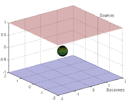
Figure 1: Sketch of the geometry for numerical simulations of shape detection and classification. 256 sources are placed on a uniform grid on the top square $[-2,2]^{2}\times\{1\}$ and 256 receivers are placed on a uniform grid on the bottom square $[-2,2]^{2}\times\{-1\}$. An unknown conductive object that has to be detected and classified lies between these two squares.

We set the values $\sigma=5.97e7$S/m, $\mu_{*}=\mu_{0}=1.2566e-06$ H/m, and $\alpha=0.01$ m, $\omega=133.5$, so that $k\alpha^{2}=1$ and the asymptotic formula form Theorem 2.1 is valid. Relevant CPTs are computed by a finite element code based on PHG [28], and we then form the product $U\mathcal{M}_{q}V_{p}$. To simulate the matrix $A$ (recall formula (4.1)), we generate an $N$ by $M$ matrix $W$ with entries from a normal distribution with mean 0 and variance 1 using the matlab function ’randn’ and we compute the sum $U\mathcal{M}_{q}V_{p}+\frac{\sigma_{\mathrm{noise}}}{\sqrt{M}}W$ for different values of $\sigma_{\mathrm{noise}}$.

Figure 2 shows the localization results. The MSR has three dominant singular values indicating that there is only one target. The functional $\mathcal{I}_{MU}$ defined in (4.4) peaks at the center of the target, as anticipated.

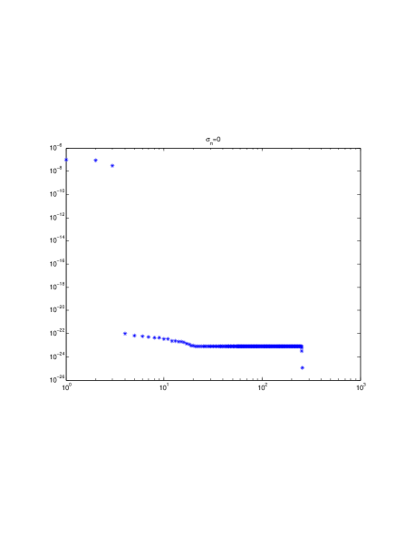
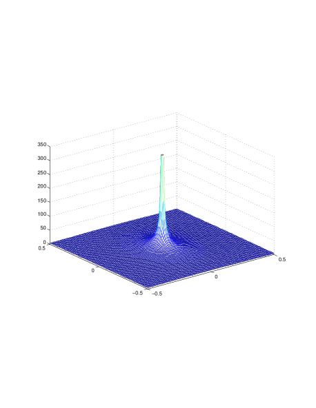
Figure 2: Finding the location of an an ellipsoidal target. The ellipsoid is defined by the equation $x^{2}+y^{2}+\frac{z^{2}}{4}\leq\alpha^{2}$, $\alpha=0.01$ m. The electromagnetic parameters are $\sigma=5.97e7$ S/m, $\mu_{*}=\mu_{0}=1.2566e-06$ H/m, $\omega=133.5$. The sources and the receivers are laid out as indicated by Figure 1. Left: log-log plot of the singular values of MSR matrix defined in (2.21) computed using approximation formula (2.22). Right: magnitude of imaging functional $\mathcal{I}_{MU}$ defined in (4.4) plotted on the $xy$ plane. As expected, this functional peaks at the center of the target.

Next, we assess how this MUSIC location algorithm is capable of differentiating two distinct targets. To do that, pick two small targets shaped as previously and centered in the $xy$ plane. Denote by ${\itbf z}_{1}$ and ${\itbf z}_{2}$ their centers, assume that ${\itbf z}_{1}$ is at the origin (accordingly the second ellipsoid is given by the equation $(x-{\itbf z}_{2}\cdot\bm{e}_{1})^{2}+(y-{\itbf z}_{2}\cdot\bm{e}_{2})^{2}+\frac{z^{2}}{4}\leq\alpha^{2}$, $\alpha=0.01$ m). These two targets have same conductivity $\sigma=5.97e7$ S/m, permeability is set to be constant everywhere $\mu_{0}=1.2566e-06$ H/m, and as previously $\omega=133.5$. In this simulation set $L$ to be a positive distance and place (on a uniform grid) 256 sources on the square $[-2,2]^{2}\times\{L\}$ 256 receivers on the square $[-2,2]^{2}\times\{-L\}$. Denote by $\sigma_{1}$ the maximum singular value of the MSR matrix without noise, that is, $U\mathcal{M}_{q}V_{p}$. We define the signal-to-noise ratio by

$$\mathrm{SNR}=\sigma_{1}/\sigma_{\mathrm{noise}},$$

and the noise level as $\mathrm{SNR}^{-1}$.

In Tables 1-5, we give for different values of $L$ the minimum distance ${\color[rgb]{0,0,0}d_{\mathrm{min}}}$ between ${\itbf z}_{1}$ and ${\itbf z}_{2}$ needed to clearly differentiate the two targets. In Figure 3, we plot the minimum distance ${\color[rgb]{0,0,0}d_{\mathrm{min}}}$ against $\mathrm{SNR}$ for $L=1.0,0.5,0.25$ in logarithmic scale. We observe that the minimum distance ${\color[rgb]{0,0,0}d_{\mathrm{min}}}$ is approximately equal to $2L\;\mathrm{SNR}^{-1/3}$.

noise level	0.1%	0.2%	0.3%	0.5%	1%	2%	3%	4%	5%	6%
${\color[rgb]{0,0,0}d_{\mathrm{min}}}$	0.27	0.33	0.37	0.43	0.53	0.63	0.68	0.74	0.78	0.84

Table 1: Computed values of ${d_{\mathrm{min}}}$, the minimum distance needed to differentiate the two ellipsoidal targets with diameter $0.02$. Here $L=1.25$, where $L$ is the distance from the targets to the plane containing the sources, which we chose to be equal to the distance from the targets to the plane containing the receivers.

noise level	0.1%	0.2%	0.3%	0.5%	1%	2%	3%	4%	5%	6%
${\color[rgb]{0,0,0}d_{\mathrm{min}}}$	0.22	0.26	0.29	0.34	0.42	0.50	0.57	0.62	0.66	0.69

Table 2: Same as previous table for $L=1$.

noise level	0.1%	0.2%	0.3%	0.5%	1%	2%	3%	4%	5%	6%
${\color[rgb]{0,0,0}d_{\mathrm{min}}}$	0.16	0.19	0.22	0.26	0.31	0.38	0.42	0.44	0.48	0.50

Table 3: Same as previous table for $L=0.75$.

noise level	0.1%	0.2%	0.3%	0.5%	1%	2%	3%	4%	5%	6%
${\color[rgb]{0,0,0}d_{\mathrm{min}}}$	0.11	0.13	0.15	0.17	0.21	0.25	0.28	0.30	0.32	0.33

Table 4: Same as previous table for $L=0.5$.

noise level	0.1%	0.2%	0.3%	0.5%	1%	2%	3%	4%	5%	6%
${\color[rgb]{0,0,0}d_{\mathrm{min}}}$	0.074	0.09	0.1	0.112	0.132	0.146	0.156	0.16	0.17	0.18

Table 5: Same as previous table for $L=0.25$.

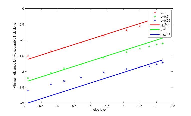
Figure 3: ${d_{\mathrm{min}}}$, the minimum distance needed to differentiate the two ellipsoidal targets with diameter 0.02, plotted as stars against the $\mathrm{SNR}$. Units are logarithmic. The solid lines illustrate the estimate ${d_{\mathrm{min}}}\sim 2L\;\mathrm{SNR}^{-1/3}$.

7.2 Performance of the classification algorithm

Next, we report some numerical results to demonstrate the efficiency of Algorithm 6.1 at a single frequency and at multiple frequencies. The dictionary includes the following domains: (1) cube $[-1,1]^{3}$, (2) cylinder $\{x^{2}+y^{2}\leq 1,-0.5\leq z\leq 0.5\}$, (3) ellipsoid $x^{2}+y^{2}+\frac{z^{2}}{4}\leq 1$, (4) L-shaped domain $[-1,1]\times[-0.5,0.5]\times[-0.5,0.5]$, (5) prism $\{-1\leq x,-1\leq y,\mbox{ and }x+y\leq 1\}\times[-1,1]$, and (6) sphere $x^{2}+y^{2}+z^{2}\leq 1$. These shapes are sketched in Figure 4.

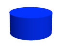
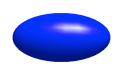
Figure 4: The shapes in the dictionary.

7.3 Classification from measurements at a single frequency

Table 6 indicates for each of the five domains listed above the three significant singular values of $\mathbb{M}$ at the operating frequency $\omega=133.5$.

shape	singular values
cube	2.2485, 2.2485, 2.2484
cylinder	0.5997, 0.5997,0.3429
ellipsoid	2.6159,2.1916,2.1916
L-shape	0.1316,0.1278,0.0941
prism	3.0423, 2.8299,2.3296
sphere	0.8282, 0.8277,0.8277

shape	singular values
cube	1.0, 1.0, 1.0
cylinder	1.0, 1.0,0.5717
ellipsoid	1.0,0.8378,0.8377
L-shape	1.0,0.9715,0.7151
prism	1.0, 0.9302,0.7657
sphere	1.0, 0.9993,0.9993

Table 6: Three significant singular values of $\mathbb{M}$ for targets with different shapes. The table on the left is for the original singular values while the table on the right is for the normalized singular values.

We first show results on classification using a single frequency ($\omega=133.5$). This frequency satisfies $k\alpha^{2}=O(1)$ so the asymptotic formula in Section 2 can be safely used. We first locate the target by applying the MUSIC algorithm. We then recover the CPT matrices by solving the minimization problem (6.2). Set $\mathcal{D}=\{D_{1},D_{2},D_{3},D_{4},D_{5},D_{6}\}$, where these shapes correspond to the aforementioned five domains labeled in the same order. Assume that the number of sources and receivers are both 256. Accordingly, the MSR matrix is $256$ by $256$. In this simulation we place these sources on a uniform grid on the square $[-2,2]^{2}\times\{1\}$ and these receivers on a uniform grid on the square $[-2,2]^{2}\times\{-1\}$: see in Figure 1 a sketch of the geometry for numerical simulations of shape detection and classification in this paper. Figure 5 shows the matching results for a target whose shape is defined by the equation $x^{2}/4+y^{2}+z^{2}\leq\alpha^{2}$. Note that this is just a rotation of the ellipsoidal target from the dictionary.

Figure 6 shows the results of classification for a small ellipsoid target described by $x^{2}+y^{2}+z^{2}/4\leq 0.25\alpha^{2}$.
It is visible on this figure that our algorithm can recognize the correct shape. We find that, at each noise level from our selection, the minimum $\min_{D\in\mathcal{D}}\{\|D-\hat{D}\|_{2}\}$ is achieved at $D=D_{3}$, that is at the ellipsoid shaped target. It is remarkable that even in the case when the noise level reaches $40\%$, we can still recognize the target.

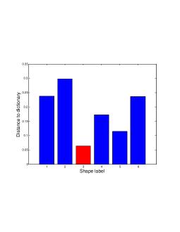
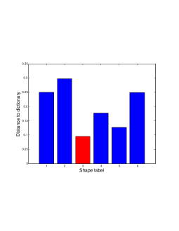
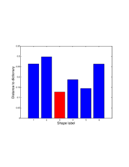
Figure 5: Matching results for a rotated ellipsoid target, from left to right, top to bottom, $nl=10\%,20\%,30\%,40\%$. Labels on horizontal axis: 1 -cube, 2 -cylinder, 3 -ellipsoid, 4 -L-shaped domain, 5 -prism, 6 -sphere. Vertical axis: distance between the shape descriptors of the target computed from the measurements and the shape descriptors of dictionary. The distance is computed by averaging 1000 realizations for each noise level.

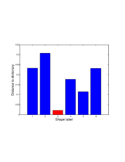
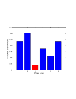
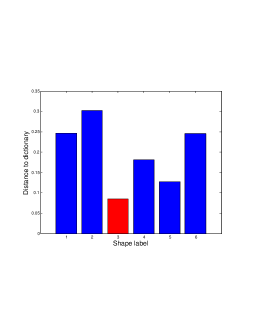
Figure 6: Matching results for a small ellipsoid target, from left to right, top to bottom, $nl=10\%,20\%,30\%,40\%$. Labels on horizontal axis: 1 -cube, 2 -cylinder, 3 -ellipsoid, 4 -L-shaped domain, 5 -prism, 6 -sphere. Vertical axis: distance between the shape descriptors of the target computed from the measurements and the shape descriptors of dictionary. The distance is computed by averaging 1000 realizations for each noise level.

7.4 Classification from measurements at multiple frequencies

In Table 6, we show that the normalized singular values for the cube and the sphere are very similar, so we can not distinguish a cube from a sphere if the data is corrupted by noise. The dependence of CPT matrix $\mathbb{M}$ on $s$ is nonlinear, in other words, $\mathbb{M}$ is nonlinear with respect to $\omega$. This motivates trying to use multiple frequencies in order to be able to differentiate them. In our simulation we used the frequencies $\omega_{n}=73.5+10n,n=1,2,\ldots,19$. The highest frequency in this range is $\omega=263.5$, yielding $k\alpha^{2}\approx 2$: the skin depth $\delta$ is close to $\alpha$ and our basic asymptotic approximation is still valid. If we keep increasing the frequency our asymptotic approximation breaks down, which physically relates to the skin effect for conductive materials. Figure 7 shows the classification results for a cube. At each noise level, we run the algorithm 1000 times and average the results. This clearly illustrates that using multiple frequencies for shape descriptors makes it possible to distinguish a cube from a sphere.

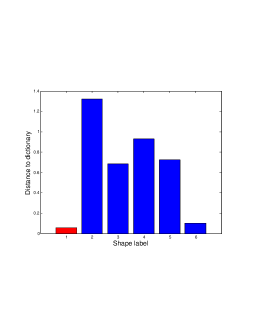
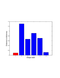
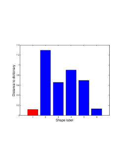
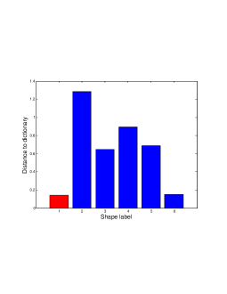
Figure 7: Use of multiple frequencies for identifying a cube. Frequencies are $\omega_{n}=73.5+10n,n=1,2,\ldots,19$, so the requirement $\nu=O(1)$ for approximation formula from Theorem 2.1 to be valid is not violated (given that we set $\sigma=5.97e7$S/m, $\mu_{*}=\mu_{0}=1.2566e-06$ H/m, and $\alpha=0.01$ m). Labels on horizontal axis: 1 -cube, 2 -cylinder, 3 -ellipsoid, 4 -L-shaped domain, 5 -prism, 6 -sphere. Vertical axis: distance between the shape descriptors of the target computed from the measurements and the shape descriptors of dictionary. The distance is computed by averaging 1000 realizations for each noise level. From left to right, top to bottom: the noise level is equal to $5\%,8\%,10\%,12\%$.

8 Concluding remarks

In this paper we have developed an efficient classification algorithm from induction data based on dictionary matching of shape descriptors. This was done under the assumption that the characteristic size of the target is of the same order of magnitude or smaller than the skin depth. The shape descriptors are constructed from conductive polarization tensors at multiple frequencies. If a target has a different magnetic permeability from the background medium, then its second polarization tensor associated with the magnetic contrast can be extracted from the data and used to better classify the target. The combined use of these two polarization tensors for classification will be the subject of a forthcoming publication. In future work, we will also investigate the effect of medium noise on the classification capabilities of our proposed multifrequency, induction based, algorithm. Our algorithm is currently limited to the case of well separated targets. Extending it to the case of clustered objects will likely prove to be quite challenging. Since that case is of great importance in some practical applications, we will certainly study it at some point in the future.

References

• [1] H. Ammari, T. Boulier, J. Garnier, W. Jing, H. Kang, and H. Wang, Target identification using dictionary matching of generalized polarization tensors, Found. Compt. Math., 14 (2014), 27–62.
• [2] H. Ammari, T. Boulier, J. Garnier, and H. Wang, Shape recognition and classification in electro-sensing, Proc. Nat. Acad. Sci., to appear, arXiv:1302.6384.
• [3] H. Ammari, T. Boulier, J. Garnier, H. Kang, and H. Wang, Tracking of a mobile target using generalized polarization tensors, SIAM J. Imag. Sci., 6 (2013), 1477–1498.
• [4] H. Ammari, A. Buffa, and J.C. Nédélec, A justification of eddy currents model for the Maxwell equations, SIAM J. Appl. Math., 60 (2000), 1805–1823.
• [5] H. Ammari, J. Chen, Z. Chen, J. Garnier, and D. Volkov, Target detection and characterization from electromagnetic induction data, J. Math. Pures Appl., 101 (2014), 54–75.
• [6] H. Ammari, J. Garnier, W. Jing, H. Kang, M. Lim, K. Sølna , and H. Wang, Mathematical and Statistical Methods for Multistatic Imaging, Lecture Notes in Mathematics, Vol. 2098, Springer-Verlag, Berlin, 2013.
• [7] H. Ammari, J. Garnier, and V. Jugnon, Detection, reconstruction, and characterization algorithms from noisy data in multistatic wave imaging, Discrete and Continuous Dynamical Systems-Series S, to appear.
• [8] H. Ammari, J. Garnier, H. Kang, M. Lim, and S. Yu, Generalized polarization tensors for shape description, Numer. Math., 126 (2014), 199–224.
• [9] H. Ammari, J. Garnier, H. Kang, W.K. Park, and K. Sølna, Imaging schemes for perfectly conducting cracks, SIAM J. Appl. Math., 71 (2011), 68–91.
• [10] H. Ammari, E. Iakovleva, D. Lesselier, and G. Perrusson, A MUSIC-type electromagnetic imaging of a collection of small three-dimensional inclusions, SIAM J. Sci. Comput., 29 (2007), 674–709.
• [11] H. Ammari and H. Kang, Reconstruction of small inhomogeneities from boundary measurements, Vol. 1846, Lecture Notes in Mathematics, Springer-Verlag, Berlin, 2004.
• [12] H. Ammari and H. Kang, Polarization and Moment Tensors: with Applications to Inverse Problems and Effective Medium Theory, Applied Mathematical Sciences, Vol. 162, Springer-Verlag, New York, 2007.
• [13] H. Ammari and A. Khelifi, Electromagnetic scattering by small dielectric inhomogeneities, J. Math. Pures Appl., 82 (2003), 749–842.
• [14] H. Ammari, M. P. Tran, and H. Wang, Shape identification and classification in echolocation, SIAM J. Imag. Sci., to appear, arXiv:1308.5625.
• [15] H. Ammari, M. Vogelius, and D. Volkov, Asymptotic formulas for perturbations in the electromagnetic fields due to the presence of inhomogeneities of small diameter II. The full Maxwell equations, J. Math. Pures Appl., 80 (2001), 769–814.
• [16] H. Ammari and D. Volkov, The leading-order term in the asymptotic expansion of the scattering amplitude of a collection of Finite Number of dielectric inhomogeneities of small diameter, Int. J. Mult. Comput. Eng., 3 (2005), 149–160.
• [17] B. A. Auld and J. C. Moulder, Review of advances in quantitative eddy current nondestructive evaluation, J. Nondest. Eval., 18 (1999), 3–36.
• [18] Y. Capdeboscq and M. S. Vogelius, A review of some recent work on impedance imaging for inhomogeneities of low volume fraction, Contemporary Mathematics, 362 (2004), 69–88.
• [19] D. J. Cedio-Fengya, S. Moskow, and M. S. Vogelius, Identification of conductivity imperfections of small diameter by boundary measurements: Continuous dependence and computational reconstruction, Inverse Problems, 14 (1998), 553–595.
• [20] P. Gao, L. Collins, P. M. Garber, N. Geng, and L. Carin, Classification of landmine-like metal targets using wideband electromagnetic induction, IEEE Trans. Geosci. Remote Sensing, 38 (2000), 1352–1361.
• [21] E. Gasperikova, J. T. Smith, H. F. Morrison, A. Becker, and K. Kappler, UXO detection and identification based on intrinsic target polarizabilities-A case history, Geophysics, 74 (2009), B1–B8.
• [22] N. Khadr, B. J. Barrow, T. H. Bell, and H. H. Nelson, Target shape classification using electromagnetic induction sensor data, Proceedings of UXO Forum 1998.
• [23] O. Kwon, J. K. Seo, and J. R. Yoon, A real time algorithm for the location search of discontinuous conductivities with one measurement, Comm. Pure Appl. Math., 55 (2002), 1–29.
• [24] J. C. Nédélec, Acoustic and Electromagnetic Equations: Integral Representations for Harmonic Problems, Springer, 2001.
• [25] S. J. Norton and I. J. Won, Identification of buried unexploded ordnance from broadband electromagnetic induction data, IEEE Trans. Geoscience Remote Sensing, 39 (2001), 2253–2261.
• [26] J. Rosell, R. Casanas, and H. Scharfetter, Sensitivity maps and system requirements for magnetic induction tomography using a planar gradiometer, Physiol. Meas., 22 (2001), 212–130.
• [27] M. S. Vogelius and D. Volkov, Asymptotic formulas for perturbations in the electromagnetic fields due to the presence of inhomogeneities of small diameter, M2AN Math. Model. Numer. Anal., 34 (2000), 723–748.
• [28] PHG, Parallel Hierarchical Grid, available at: http://lsec.cc.ac.cn/phg/