Precious Metals in SDSS Quasar Spectra II: Tracking the Evolution of Strong, $0.4<z<2.3$ Mg II Absorbers with Thousands of Systems

Abstract

We have performed an analysis of over 34,000 Mg II doublets at $0.36<z<2.29$ in Sloan Digital Sky Survey (SDSS) Data-Release 7 quasar spectra; the catalog, advanced data products, and tools for analysis are publicly available. The catalog was divided into 14 small redshift bins with roughly 2500 doublets in each, and from Monte-Carlo simulations, we estimate 50% completeness at rest equivalent width $W_{\rm r}\approx 0.8\,\mbox{\AA}$. The equivalent-width frequency distribution is described well by an exponential model at all redshifts, and the distribution becomes flatter with increasing redshift, i.e., there are more strong systems relative to weak ones. Direct comparison with previous SDSS Mg II surveys reveal that we recover at least 70% of the doublets in these other catalogs, in addition to detecting thousands of new systems. We discuss how these surveys come by their different results, which qualitatively agree but, due to the very small uncertainties, differ by a statistically significant amount. The estimated physical cross-section of Mg II-absorbing galaxy halos increased three-fold, approximately, from $z=0.4\rightarrow 2.3$, while the $W_{\rm r}\geq 1\,\mbox{\AA}$ absorber line density grew, $d\mathcal{N}_{\mathrm{Mg\,II}}/dX$, by roughly 45%. Finally, we explore the different evolution of various absorber populations—damped Lyman-$\alpha$ absorbers, Lyman-limit systems, strong C IV absorbers, and strong and weaker Mg II systems—across cosmic time ($0<z<6$).

1. Introduction

The cosmic enrichment cycle describes the movement of gas and heavy elements (or metals) from the sites of star formation in galaxies into the intergalactic medium (IGM) and potentially back again. An understanding of gas surrounding galaxies—or the circum-galactic medium (CGM)—is crucial to understanding feedback and gas accretion processes. Mg II $\lambda\lambda 2796,2803$ absorption-line surveys—in both quasar and galaxy spectra—have long been utilized to characterize enriched, photoionized gas clouds within and surrounding galaxies (e.g., Bergeron, 1986; Lanzetta et al., 1987; Sargent et al., 1988; Petitjean & Bergeron, 1990; Steidel & Sargent, 1992; Churchill et al., 1999; Weiner et al., 2009; Martin & Bouché, 2009; Bordoloi et al., 2011; Lovegrove & Simcoe, 2011; Kacprzak et al., 2011a; Kornei et al., 2012; Churchill et al., 2013; Rubin et al., 2013).

Mg II is a strong transition for a wide range of ionization parameters, even with a modest number of Mg atoms, making it a common and well-studied ion. The metallicities of Mg II systems, at $0.4<z<1.8$, range from one-tenth to super-solar (Rigby et al., 2002; Charlton et al., 2003; Misawa et al., 2008). Ground-based, optical spectrographs can detect the Mg II doublet over $0.1\lesssim z\lesssim 2.5$; infrared spectroscopy can extend that range to $z\approx 5.5$. Mg II absorption-line surveys take on three flavors: (i) galaxy self-absorption; (ii) galaxies or quasars probing galaxies; and (iii) quasar absorption-line (QAL) spectroscopy. Results from all experimental setups provide evidence that Mg II absorption traces the CGM, though only the first two methods identify the host galaxies explicitly.

Strong Mg II absorbers, with rest equivalent widths of the 2796 Å line $W_{\rm r}{}_{,\mathrm{2796}}\gtrsim 1\,\mbox{\AA}$, have been linked to massive, star-forming galaxies, possibly arising in their starburst-driven outflows (Bouché et al., 2006; Weiner et al., 2009; Rubin et al., 2010). In this model, Mg II absorption is found in cool, interlaced clumps within a heated galactic outflow. Recent results show that the strength of the Mg II absorption depends on the azimuthal angle relative to the host galaxies (Bordoloi et al., 2011; Bouché et al., 2012; Kacprzak et al., 2012). Under the model of a biconical starburst-driven outflow, the stronger Mg II absorbers are detected over the plane of the disk. Both studies detect weak Mg II absorption at large azimuthal angles (i.e., along the disk axis), and these systems may trace inflowing material (Chen et al., 2010b), possibly co-rotating with the disk (Kacprzak et al., 2011b).

Early-type galaxies also host Mg II systems (Chen et al., 2010a; Gauthier et al., 2010; Gauthier & Chen, 2011), and they tend to be weaker than absorbers around star-forming galaxies (Bowen & Chelouche, 2011), which supports the idea that weak systems may trace gas accretion or at least the “ambient” CGM. Gauthier et al. estimate the covering fraction of Mg II absorption to be $\approx\!14\%$ for massive luminous red galaxies and greater for less massive galaxies. Chen et al. (2010a) searched for absorbers in quasar sightlines near galaxies (as opposed to seeking galaxies near sightlines with known Mg II systems) and found no correlation to the star-formation rate of the host galaxies. They traced the absorption in bright, field galaxies out to about 100$\,\mathrm{kpc}$ with 50–80% covering fraction.

Gauthier (2013) propose that ultra-strong, $W_{\rm r}{}_{,\mathrm{2796}}\gtrsim 3\,\mbox{\AA}$ Mg II systems trace gas in galaxy groups (though see Nestor et al., 2011). The ultra-strong Mg II absorbers have broad, kinematically complex profiles. Galaxies in groups may have different radial $W_{\rm r}{}_{,\mathrm{2796}}$ profiles from isolated galaxies (Chen et al., 2010a).

Mg II absorption has been used to select damped $\mathrm{Ly}\alpha$ absorber (DLA) candidates at $z\lesssim 1.6$, because it is a common transition for even moderately metal-enriched gas and can be observed with ground-based optical spectrographs (Rao & Turnshek, 2000), whereas the distinctive $\mathrm{Ly}\alpha$ profile is accessible only with space-based ultraviolet spectrographs. DLAs, with H I column densities $\log N_{\rm H\,I}\geq 20.3$, are considered the cold gas reservoirs for star formation and thought to reside in star-forming galaxies (see Wolfe et al., 2005, and references therein).

The large database of quasar spectra generated by SDSS (York et al., 2000) provides a way to efficiently find strong Mg II systems in the range $0.4<z<2.3$, or from when the universe was 9.5 Gyr to 3 Gyr old. At SDSS resolution ($\approx\!150\,{\rm km\,s}^{-1}$) and typical signal-to-noise, SDSS is more complete at $W_{\rm r}{}_{,\mathrm{2796}}\gtrsim 1\,\mbox{\AA}$, defining “strong” Mg II absorbers. There have been four SDSS Mg II surveys in: the early data release or EDR—Nestor et al. (2005, hereafter N05); DR3—Prochter et al. (2006a, P06); DR4—Quider et al. (2011, Q11); and DR7—Zhu & Ménard (2013, ZM13).

Most of these studies measured the frequency distribution of $W_{\rm r}{}_{,\mathrm{2796}}$ and the absorber redshift density, $d\mathcal{N}_{\mathrm{Mg\,II}}/dz$. The former is fit well by an exponential model, showing that there is a break in the full equivalent-width distribution, when accounting for the weaker systems being well-modeled by a power-law distribution (Churchill et al., 1999; Narayanan et al., 2007). For $W_{\rm r}{}_{,\mathrm{2796}}\geq 1\,\mbox{\AA}$, $d\mathcal{N}_{\mathrm{Mg\,II}}/dz$ increases by a factor of $\approx\!2.5$ from $z\approx 0.4\rightarrow 2.3$. Recent results from an infrared survey showed that $d\mathcal{N}_{\mathrm{Mg\,II}}/dz$ decreases from $z\approx 2\rightarrow 5.5$ (Matejek & Simcoe, 2012).

P06 first connected the Mg II evolution to the cosmic star-formation rate density, $\rho_{\ast}$, and Ménard et al. (2011) constructed an empirical relation between $d\mathcal{N}_{\mathrm{Mg\,II}}/dz$ and $\rho_{\ast}$, which peaks at $z\approx 2$ to 3 and roughly matches the $d\mathcal{N}_{\mathrm{Mg\,II}}/dz$ evolution (Matejek & Simcoe 2012, ZM13). Though QAL surveys do not produce direct ties between Mg II absorbers and galaxies, the seemingly related evolution of $d\mathcal{N}_{\mathrm{Mg\,II}}/dz$ for $W_{\rm r}{}_{,\mathrm{2796}}\geq 1\,\mbox{\AA}$ and $\rho_{\ast}$ is at least circumstantial evidence that strong Mg II systems are linked to star formation. Also, Ménard et al. (2011) detected [O II] $\lambda 3727$ nebular emission in the SDSS fibers with Mg II absorption, which directly ties the absorption to star formation.

Matejek & Simcoe (2012) observed little evolution in $d\mathcal{N}_{\mathrm{Mg\,II}}/dz$ for $0.3\,\mbox{\AA}\leq W_{\rm r}{}_{,\mathrm{2796}}<1\,\mbox{\AA}$ systems over $0.4\lesssim z_{2796}\lesssim 5.5$, comparing to N05 and later upheld by ZM13. This suggests a population of weak Mg II absorbers being established early in the history of the universe or being constantly replenished, at a conserving rate, over time.

In spite of the numerous observations of Mg II absorbers and their direct or inferred relationship with galaxies, the origin of the absorbing gas in the CGM is not yet clearly understood. We are motivated to conduct a SDSS Mg II survey so that we may fairly compare the results with our high-redshift results (Matejek & Simcoe, 2012) and with our other SDSS metal-line surveys. We have completed the search for C IV $\lambda\lambda 1548,1550$ (Cooksey et al., 2013, hereafter, Paper I), and our survey of Si IV $\lambda\lambda 1393,1402$ is in preparation. We also discuss why the various SDSS Mg II surveys produce different results, which, due to the large sample sizes, are statistically significant.

We summarize how we construct our Mg II catalog, correct for completeness, and compare with previous SDSS catalogs in Section 2, while absorber-by-absorber comparisons are left to Appendix A. The main results are detailed in Section 3. We discuss the implications of our results in the context of the CGM and the results from surveys of other absorber populations in Section 4. The summary is given in Section 5. We adopt the WMAP5 cosmology: $H_{0}=71.9\,{\rm km\,s}^{-1}\,\mathrm{Mpc}^{-1}$, $\Omega_{\rm M}=0.258$, and $\Omega_{\Lambda}=0.742$ (Komatsu et al., 2009).

Table 1Sightline Summary

(1)	(2)	(3)	(4)	(5)	(6)	(7)	(8)	(9)	(10)
QSO ID	R.A.	Decl.	$z_{\rm QSO}$	$\langle{\rm S/N}\rangle$	$f_{\rm BAL}$	$\Delta X_{\rm max}$	$\mathcal{N}_{\rm cand}$	$\mathcal{N}_{\rm Mg\,II}$	$\delta X_{\rm Mg\,II}$
				(pixel-1)
52203-0685-467	00:00:06.53	+00:30:55.2	1.8246	7.85	0	4.04	0	0	$\cdots$
52203-0685-470	00:00:08.13	+00:16:34.6	1.8373	10.34	0	2.27	0	0	$\cdots$
52235-0750-082	00:00:09.38	+13:56:18.4	2.2342	4.17	0	0.19	2	0	$\cdots$
52143-0650-199	00:00:09.42	–10:27:51.9	1.8449	8.54	0	3.33	2	1	0.028
52235-0750-499	00:00:11.41	+14:55:45.6	0.4597	7.83	0	0.49	0	0	$\cdots$
51791-0387-200	00:00:11.96	+00:02:25.3	0.4789	11.16	0	1.64	0	0	$\cdots$
52235-0750-098	00:00:13.14	+14:10:34.6	0.9582	12.26	0	2.15	0	0	$\cdots$
52203-0685-198	00:00:14.82	–01:10:30.7	1.8877	9.21	0	2.87	0	0	$\cdots$
52203-0685-439	00:00:15.47	+00:52:46.8	1.8516	7.22	0	2.47	2	0	$\cdots$
52991-1489-142	00:00:16.43	–00:18:33.3	0.7030	6.20	0	0.92	0	0	$\cdots$
52143-0650-459	00:00:17.38	–08:51:23.7	1.2491	7.44	0	3.74	1	0	$\cdots$

Note. — Column 1 is the adopted QSO identifier from the spectroscopic modified Julian date, plate, and fiber number. Columns 2 through 4 are from the DR7 QSO catalog (Schneider et al., 2010). Column 5 is the median S/N measured in the region searched for Mg II. The binary BAL flag $f_{\rm BAL}$ in Column 6 indicates which sightlines were considered BALs by at least one author (4) and which were confirmed by the authors as BALs to exclude (8). Column 7 is the maximum co-moving pathlength available in the sightline. Columns 8 and 9 give the number of candidate and confirmed Mg II doublets, respectively. Column 10 is the pathlength blocked by the $\mathcal{N}_{\rm Mg\,II}$ doublets in the sightline. (This table is available in a machine-readable form in the online journal. A portion is shown here for guidance regarding its form and content.)

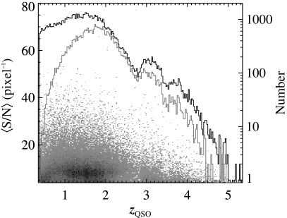
Figure 1.— Redshift and $\langle{\rm S/N}\rangle$ distribution of sightlines. Using the left-hand axis, the 2D histogram shows the median signal-to-noise and $z_{\rm QSO}$ space of the analyzed 79,294 spectra. The black and gray histograms give the redshift distribution for all spectra and for the 28,938 with confirmed Mg II absorbers, respectively (right-hand axis).

2. Constructing the Mg II Catalog

2.1. From Quasar Spectra to Visually Verified Sample

Our Mg II absorber catalog was constructed using a subset of the SDSS DR7 quasar catalog (Schneider et al., 2010) and following an equivalent methodology to the C IV survey described in detail in Paper I, to which the interested reader is referred. Here we briefly outline the procedure.

Of the 105,783 DR7 quasar spectra, 79,595 were searched for Mg II systems (Table 1) because they: (i) were not broad absorption-line (BAL) QSOs (identified by Shen et al., 2011) and (ii) had median signal-to-noise ratio $\langle{\rm S/N}\rangle\geq 4\,{\rm pixel}^{-1}$ in the region covering intergalactic Mg II absorption (i.e., observed wavelengths greater than $1250\,\mbox{\AA}(1+z_{\rm QSO})$ and $\delta v_{\rm QSO}<-3000\,{\rm km\,s}^{-1}$). A further 301 sightlines were later excluded as “visual” BAL QSOs, leaving a total of 79,294 quasar spectra included in this survey; their distribution in $z_{\rm QSO}$–$\langle{\rm S/N}\rangle$ space is shown in Figure 1.

Every quasar spectrum was normalized with its “hybrid continuum,” a fit combining principle-component analysis, b-spline correction, and pixel/absorption-line rejection. Absorption-line candidates were automatically detected by convolving the normalized flux and error arrays with a Gaussian kernel with a full-width at half-maximum of one pixel, roughly an SDSS resolution element (resel). Candidate Mg II doublets were identified based solely on the characteristic velocity separation ($767\,{\rm km\,s}^{-1}$), plus/minus $150\,{\rm km\,s}^{-1}$ to allow for blending. The candidate doublets had convolved $({\rm S/N})_{\rm conv}\geq 3.5\,{\rm resel}^{-1}$ in the 2796 Å line and $2.5\,{\rm resel}^{-1}$ in the 2803 Å line. Any automatically detected absorption feature with $({\rm S/N})_{\rm conv}\geq 3.5\,{\rm resel}^{-1}$ and broad enough to enclose a Mg II doublet was included in the candidate list.

The wavelength bounds of the absorption lines were automatically defined by where the convolved S/N array began increasing when stepping away from the automatically detected line centroid. The new centroid was then set as the flux-weighted average wavelength within the bounds, and the Mg II doublet redshift, $z_{2796}$, was defined by the new 2796 Å centroid.

From simulations of synthetic Mg II profiles with known equivalent widths, we empirically determined that capping the flux at the continuum plus one sigma (Poisson uncertainty of the flux and continuum error) yielded the most accurate $W_{\rm r}$ measurements using the technique of boxcar summation; the measured $W_{\rm r}$ was 0.08 Å larger than the input $W_{\rm r}$(in the median), with a median absolute deviation of 0.21 Å. Hence, our (observed) equivalent widths are the sum of this modified absorption within the wavelength bounds (i.e., $(1-f)\delta\lambda$).

All candidates were visually inspected by at least one author and most by two. They were rated on a four-point scale from 0 (definitely false) to 3 (definitely true). The systems were judged largely on the Mg II doublet (e.g., centroid alignment, correlated profiles) but possibly associated ions were also reviewed to aid verification. All Mg II absorbers with rating of 2 or 3 were included in subsequent analyses and combined into systems if separated by less than $250\,{\rm km\,s}^{-1}$.

Ultimately, we detected 35,629 doublets—from over 90,000 candidates—with $W_{\rm r}{}_{,\mathrm{2796}}<9\,\mbox{\AA}$ and $0.36<z_{2796}<2.29$ (Table 2). We excluded the C IV emission-line region, $\pm 3000\,{\rm km\,s}^{-1}$ around $1548.195\,\mbox{\AA}(1+z_{\rm QSO})$, because the continuum fits in this region were questionable, owing to the potentially large velocity offsets of the emission lines and the large incidence of strong intrinsic absorption. In addition, real intervening Mg II absorption could be lost in the intrinsic C IV absorption, thus hindering the recovery of Mg II systems in this region. This reduced the total sample size by 531. We also limit our sample to systems with $\delta v_{\rm QSO}<-5000\,{\rm km\,s}^{-1}$, leaving 34,254 doublets for further analyses.

Table 2Mg II System Summary

(1)	(2)	(3)	(4)		(5)		(6)
QSO ID	$z_{\rm QSO}$	$z_{2796}$	$W_{\rm r}{}_{,\mathrm{2796}}$		$W_{\rm r}{}_{,\mathrm{2803}}$		$C(W_{\rm r}{}_{,\mathrm{2796}})$
			(Å)		(Å)
52235-0750-082	2.2342	0.96363	2.445 $\pm$	0.174	1.547 $\pm$	0.168	0.915 $\pm$	0.006
		1.14500	0.268 $\pm$	0.115	0.254 $\pm$	0.143	0.112 $\pm$	0.069
52143-0650-199	1.8449	1.31252	1.965 $\pm$	0.235	2.016 $\pm$	0.198	0.882 $\pm$	0.034
		1.52824	0.394 $\pm$	0.159	0.507 $\pm$	0.180	0.203 $\pm$	0.113
52203-0685-439	1.8516	1.37148	0.650 $\pm$	0.212	1.140 $\pm$	0.253	0.400 $\pm$	0.163
		1.63660	1.457 $\pm$	0.577	2.376 $\pm$	0.396	0.789 $\pm$	0.249
52143-0650-459	1.2491	0.69284	0.575 $\pm$	0.162	0.486 $\pm$	0.164	0.344 $\pm$	0.126
54389-2822-318	1.1560	0.48941	2.724 $\pm$	0.384	2.534 $\pm$	0.375	0.924 $\pm$	0.012
51791-0387-167	2.1249	1.07105	0.801 $\pm$	0.256	0.631 $\pm$	0.240	0.495 $\pm$	0.174
51791-0387-531	0.9511	0.49645	0.310 $\pm$	0.115	0.678 $\pm$	0.132	0.142 $\pm$	0.074
54389-2822-339	1.4446	0.38268	1.006 $\pm$	0.555	1.684 $\pm$	0.564	0.600 $\pm$	0.352
		0.76378	2.117 $\pm$	0.309	1.581 $\pm$	0.304	0.898 $\pm$	0.038
		1.09345	0.852 $\pm$	0.387	1.036 $\pm$	0.406	0.526 $\pm$	0.268
52143-0650-178	2.6404	1.05622	1.749 $\pm$	0.141	1.283 $\pm$	0.172	0.851 $\pm$	0.025
		1.38095	0.793 $\pm$	0.113	0.619 $\pm$	0.116	0.490 $\pm$	0.071
52251-0751-355	1.4115	0.89761	1.749 $\pm$	0.297	1.799 $\pm$	0.290	0.852 $\pm$	0.064
51791-0387-093	1.8973	1.02077	0.723 $\pm$	0.172	0.791 $\pm$	0.214	0.446 $\pm$	0.120

Note. — For each sightline (identified in Columns 1 and 2), every confirmed doublet is listed by the redshift of its Mg II 2796 line (Column 3). The rest equivalent widths of the Mg II lines are given in Columns 4 and 5. In Column 6, we give the completeness fraction for the doublet from the whole survey average. (This table is available in a machine-readable form in the online journal. A portion is shown here for guidance regarding its form and content.)

$\begin{array}[]{cc}\includegraphics[width=203.80193pt]{fig2a.pdf}&\includegraphics[width=203.80193pt]{fig2b.pdf}\end{array}$

Figure 2.— Biases of visual verification and trends of spurious detections. Left: We tested the “user bias” by rating fake $\lambda\lambda 2795,2801$ doublets that were injected and automatically recovered as candidates. The four panels show the completeness of our ability to correctly rate true doublets, as a function of redshift, spectrum $\langle{\rm S/N}\rangle$, and equivalent width in three redshift bins. The redshift cuts (vertical lines) were determined by changes in $C_{\rm user}(z_{2795})$ and to align with the closest redshift bins used in our analyses. The solid and dashed lines are the best-fit model, $C_{\rm user}(W_{\rm r})=C_{0}(1-\exp(\beta(W_{\rm r}-W_{0})))$, and its 1-$\sigma$ errors. Right: We plot the accepted false-positive fraction as functions of redshift, signal-to-noise, and equivalent width. These spurious pairs of lines were not injected but were automatically recovered. The lower panels show the best-fit model and errors to the accepted spurious fraction over $W_{\rm r}{}_{,\mathrm{2795}}$.

2.2. Testing and Correcting for Completeness

As in Paper I, we test our survey completeness with Monte-Carlo simulations. Ultimately, our completeness fractions, $C(z,W)$, are the ratios of the number of accepted (i.e., visually verified), simulated doublets, $\mathcal{N}_{\rm accept}$, to the number input, $\mathcal{N}_{\rm input}$, as a function of $z_{2796}$ and $W_{\rm r}{}_{,\mathrm{2796}}$. We estimate $C(z,W)$ in four steps, described below.

First, in a “basic” completeness test, we measured the number, $\mathcal{N}_{\rm rec}$, of simulated Mg II doublets recovered by our automated procedures, from continuum fitting to candidate selection. We generated a library of synthetic profiles, inserted them into a representative subset of sightlines, and tracked which profiles were automatically recovered. The simulated doublets reflected the observed variety in our SDSS Mg II catalog. By construction, they uniformly spanned $0.05\,\mbox{\AA}\leq W_{\rm r}{}_{,\mathrm{2796}}<6.5\,\mbox{\AA}$ but $\approx\!20\%$ sampled 6.5 Å–8 Å with decreasing frequency. We injected 1000 simulated doublets in 30% of the sightlines at a rate of $d\mathcal{N}/dz=5$. The tested sightlines sampled the entire $z_{\rm QSO}$–$\langle{\rm S/N}\rangle$ space, and the un-sampled sightlines were assigned the mean completeness fraction of the tested sample in small bins of $z_{\rm QSO}$ and $\langle{\rm S/N}\rangle$.

Second, we estimated the “user” bias, resulting from our visual verification. We determined the rate at which we accepted real doublets (“true positives”) and spurious pairs (“accepted false positives”); the latter are chance alignments and/or noise fluctuations. As in Paper I, we injected simulated fake doublets, with rest wavelength comparable to Mg II but with characteristic separation of 652$\,{\rm km\,s}^{-1}$, and visually rated the recovered candidates, thus measuring the accepted number, $\mathcal{N}_{\rm accept}$. Effectively, the completeness fraction is now:

$$C(z,W)=\frac{\mathcal{N}_{\rm rec}(z,W)}{\mathcal{N}_{\rm input}(z,W)}\frac{\mathcal{N}_{\rm accept}(z,W)}{\mathcal{N}_{\rm rec}(z,W)}{\rm.}$$ (1)

However, as in Paper I, we fitted a functional form to the accepted-to-recovered fraction, $C_{\rm user}(z,W)=C_{0}(1-\exp(\beta(W_{\rm r}-W_{0})))$. This adjustment slightly increased the total completeness fraction measured in the “basic” test.

We injected $\mathcal{N}_{\rm input}=16,209$ fake doublets with $W_{\rm r}<2\,\mbox{\AA}$ and $\delta v_{\rm QSO}<-5000\,{\rm km\,s}^{-1}$, and $\mathcal{N}_{\rm rec}=10,258$ were automatically recovered. Of these, we correctly rated $\mathcal{N}_{\rm accept}=8472$. The automatically generated candidate list included any pair of lines with separations within $\pm 150\,{\rm km\,s}^{-1}$ (see Section 2.1) of the fake doublet separation, which brought forth true fake doublets, real Mg II systems, and common contaminants. These contaminating pairs of lines intrinsically had a range of separations—fixed, if they are from the same system, or random, if a pair of spurious lines. Thus the $652\pm 150\,{\rm km\,s}^{-1}$ search window was sampled by a distribution very representative of contaminants affecting the Mg II survey.

As shown in Figure 2 (left panels), the user completeness generally decreases with increasing redshift and decreasing spectrum $\langle{\rm S/N}\rangle$ and $W_{\rm r}$. We divide the $C_{\rm user}$ fit at $z=0.63$ and $z=1.78$, where $C_{\rm user}$ changes rapidly and which align with our fixed bins.

Third, we scaled the completeness by the fraction of the total co-moving path length not blocked by doublets with greater $W_{\rm r}$ in the given redshift bin. All Mg II lines blocked less than 1% of the total survey path length (Table 2). This correction slightly decreased the total completeness fraction. To measure the unblocked co-moving path length available in our survey, we multiply $C(W)$ by the total path available in the given redshift bin (Figure 3).

Fourth, the user completeness tests enabled measurement of the accepted false-positive rate, $d\mathcal{N}_{\mathrm{afp}}/dX$. There were 5802 spurious candidates from the automated search, of which we incorrectly accepted 678. As shown in Figure 2 (right panels), the accepted false-positive fraction is roughly constant at $\approx 10\%$ as a function of redshift and signal-to-noise. However, the fraction increases with increasing $W_{\rm r}$, plateauing to $\approx\!10\%$ at $z<1.78$ and $\approx\!20\%$ at higher redshift. For $W_{\rm r}\geq 1\,\mbox{\AA}$, we estimate $d\mathcal{N}_{\mathrm{afp}}/dX=0.0015$ ($z<0.63$), 0.0020 ($0.63\leq z<1.78$), and 0.0045 ($z\geq 1.78$). We explain how we adjust for the accepted false-positive rate in Section 3.

As mentioned previously, we excluded the $\pm 3000\,{\rm km\,s}^{-1}$ around the quasar C IV emission line. This reduced the pathlength by 7% over $1.48\leq z<1.78$ and less (2%–5%) in other noticeably affected bins, $1.20\leq z<2.29$.

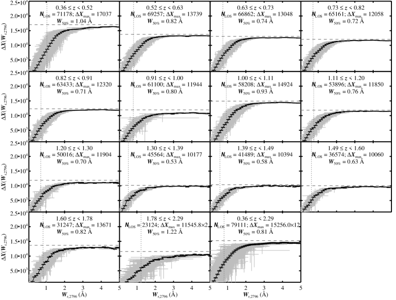
Figure 3.— Results from Monte-Carlo completeness tests. The completeness-corrected co-moving path length as a function of rest equivalent width, $\Delta X(W_{\rm r}{}_{,\mathrm{2796}})$, is shown for the 15 redshift bins used in the current study. The black lines and errors are the completeness curves, and the gray points and errors are the observations. The horizontal, dashed line traces the maximum path length available in the bin, and the vertical, dotted line indicates the equivalent width where we are 50% complete.

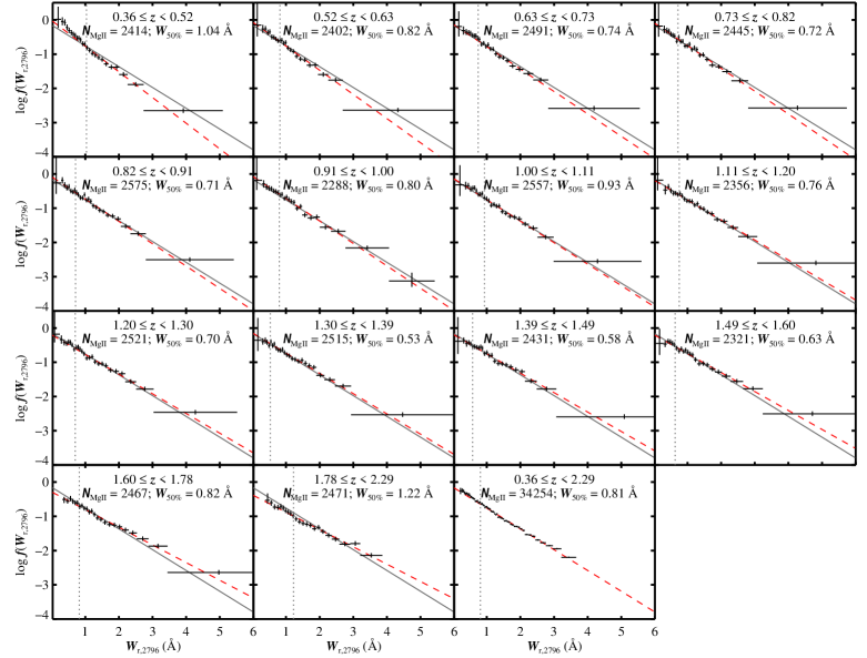
Figure 4.— Equivalent-width frequency distributions. The maximum likelihood fits of an exponential function are the dashed (red) lines, for each redshift bin, and the solid (gray) line, for the full sample. There is distinct evolution with redshift: $f(W_{\rm r})$ flattens (larger fraction of strong absorbers) and increases (more absorbers overall) with increasing redshift. The observations have been completeness corrected, and the redshift-specific 50% completeness limits are the vertical dotted lines.

2.3. Comparing with Previous SDSS Mg II Catalogs

There have been four Mg II surveys using different SDSS data releases: early (Nestor et al., 2005); third (Prochter et al., 2006a); fourth (Quider et al., 2011); and seventh (Zhu & Ménard, 2013). The surveys have a variety of differences that contribute to variations between line lists for the same subset of quasars and, hence, the results (e.g., $d\mathcal{N}_{\mathrm{Mg\,II}}/dX$), which we discuss in Section 3. Here we summarize the differences in catalogs and methodologies—from continuum fitting to final doublet selection; we leave the detailed absorber-to-absorber comparisons to Appendix A.

N05 and Q11 model the intrinsic quasar spectra with a combination of cubic splines and Gaussian profiles for emission lines, while P06 use b-splines and principle-component analysis (PCA) for emission lines. ZM13 and this study use PCA for both continua and emission lines and correct for low-frequency modulations automatically in post-processing.

All catalogs are visually verified, except for ZM13. The latter uses the Q11 catalog as their training set, and Q11, in turn, is based on the methodologies of N05. These three studies model the absorption lines with a (single or double) Gaussian profile, from which they measure the equivalent widths. These three studies and our work agree well on $W_{\rm r}{}_{,\mathrm{2796}}$ values.

Our automated candidate doublet search is based on the algorithm used by P06. We both use boxcar summation to measure equivalent widths, but P06 fix the box width, while we let it vary automatically depending on the profile. The fixed width contributes to the disagreement in our equivalent-width measurements, with P06 underestimating $W_{\rm r}{}_{,\mathrm{2796}}$. More importantly, the continuum placement in P06 was biased low by the strong absorption systems, systematically reducing their equivalent widths.

All surveys estimate their sample completeness, and all but Q11 use Monte-Carlo simulations in a similar fashion to ours, though number of realizations, types of profiles, etc. differ. Q11 relied on the tests of the automated algorithms that N05 conducted and assessed their false-negative rate by having two authors visually verify a small number of sightlines. Q11 focused on describing their catalog, and any analyses did not rely on correcting for completeness.

To summarize, the detailed catalog-to-catalog comparisons (Appendix A), we recover over 76% of the P06 absorbers, 80% of Q11, and 72% of ZM13. We can also identify why we do not recover the remaining doublets, with reasons ranging from the Shen et al. (2011) BAL QSO spectra were not searched to the line was not automatically detected by our algorithms in our normalized spectra. All catalogs are less complete for weaker systems, and each catalog’s unmatched sample largely has $W_{\rm r}{}_{,\mathrm{2796}}\lesssim 1\,\mbox{\AA}$.

Statistically and intuitively, disagreement at low equivalent width—where all surveys become highly incomplete—is expected. For example, we are 50% complete at $W_{\rm r}{}_{,\mathrm{2796}}\approx 0.8\,\mbox{\AA}$, while ZM13 is roughly 60% complete, so we should only agree on $\approx\!30\%$ of doublets of this strength. There is a large caveat because we all use SDSS spectra: our surveys are not statistically independent. However, continuum placement factors strongly into the automated detection of weak lines, which is why we attempt to quantify this affect by refitting the continua in our Monte-Carlo completeness tests.

In all cases, we detect Mg II systems not in other catalogs. Since P06 applied a hard $W_{\rm r}{}_{,\mathrm{2796}}\geq 1\,\mbox{\AA}$ cut, the vast majority of our unique systems are at lower equivalent widths, but their redshift distribution typically follows the full sample. The P06-only sample favors higher redshifts where sky lines are abundant and make verification difficult.

The redshifts of the Q11- and ZM13-only samples are a fair sampling of the full (parent) samples. However, our unique sample favors lower redshift. The effect is more pronounced with respect to ZM13, which limited the search to $\Delta z\geq 0.02$ red-ward of the quasar C IV emission line.

Another point of comparison is the $W_{\rm r}{}_{,\mathrm{2796}}/W_{\rm r}{}_{,\mathrm{2803}}$ ratio. For the matched samples, we tend to measure larger ratios than Q11 and significantly larger than ZM13; P06 did not publish $W_{\rm r}{}_{,\mathrm{2803}}$ measurements. Our unique sample has a significant number of systems with ratios less than unity, indicating we identify more blended systems.

In Section 3, we compare our science results with the published catalogs, where such comparisons are suitable.

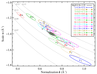
Figure 5.— Best-fit $f(W_{\rm r})$ parameters and errors. We fitted the frequency distribution with an exponential function. The best-fit normalization $k$ and scale $\alpha$ and the 1-$\sigma$ error ellipses are plotted for the 14 small redshift bins (numbered points); the 1, 2, and 3-$\sigma$ contours are shown for the fit to the full sample (black ellipses). The best-fit parameters evolve fairly smoothly with redshift, as seen by comparing the ellipses with the constant $d\mathcal{N}_{\mathrm{Mg\,II}}/dX$ curves (gray, dashed lines; see Equation 3).

3. Results

Typically, we analyzed our Mg II catalog as a whole and in 14 small redshift bins with roughly 2500 doublets each. As necessary, we modify the redshift binning to match other samples when comparing to their results.

3.1. Frequency Distribution

The equivalent-width frequency distribution $f(W_{\rm r})$ (sometimes written, $d^{2}\mathcal{N}_{\mathrm{Mg\,II}}/dW_{\rm r}/dX$) is the number of detections $\mathcal{N}_{\rm obs}(W_{\rm r})$ per rest equivalent width bin $\Delta W_{\rm r}$, per the total co-moving path length available, in the given equivalent-width bin, $\Delta X(W_{\rm r})$:

$$f(W_{\rm r})=\frac{\mathcal{N}_{\rm obs}(W_{\rm r})}{\Delta W_{\rm r}\,\Delta X(W_{\rm r})}{\rm,}$$ (2)

and it is $\Delta X(W_{\rm r})$ that accounts for completeness. We modeled $f(W_{\rm r})$ with an exponential, $f(W_{\rm r})=k\exp(\alpha W_{\rm r})$, and fitted with the maximum likelihood method of Cooksey et al. (2010) for $W_{\rm r}{}_{,\mathrm{2796}}\geq 0.8\,\mbox{\AA}$, though the results are relatively insensitive to a change of $\pm 0.2\,\mbox{\AA}$. The exponential model is a very good description of the data (Figure 4), and the best-fit parameters are given in Table 3.

The frequency distribution flattens with increasing redshift, meaning there are more strong absorbers relative to weak ones, from $z_{2796}=0.4\rightarrow 2.3$. The relatively smooth and significant evolution in the best-fit parameters from low-to-intermediate redshift can be seen in Figure 5. We also show that the line density is lower at the extrema of the redshift range, where:

$$\frac{\displaystyle d\mathcal{N}_{\mathrm{Mg\,II}}}{\displaystyle dX}\bigg{|}_{\rm fit}=\frac{\displaystyle-k}{\displaystyle\alpha}e^{\alpha W_{\rm lim}}{\rm,}$$ (3)

from the integral of the frequency distribution from a limiting equivalent width, $W_{\lim}$, to infinity.

For Mg II, the normalization ($k$) increases by a factor of $\approx\!2.5$ from $z=2.3\rightarrow 0.4$, while the scale ($\alpha$) decreases by approximately 20%. In comparison, for C IV, $\alpha$ evolves little from $z=4.5\rightarrow 1.5$, while $k$ increases by three-fold, roughly (Paper I).

As in Paper I, we factor in the accepted false-positive rate by scaling the original, measured frequency distribution, $f_{0}(W_{\rm r})$:

$$f(W_{\rm r})=\bigg{(}1-\frac{\displaystyle d\mathcal{N}_{\mathrm{afp}}/dX}{\displaystyle d\mathcal{N}_{\mathrm{Mg\,II}}/dX}\bigg{)}f_{0}(W_{\rm r}){\rm,}$$ (4)

which results in an updated best-fit normalization of:

$$k=\bigg{(}1-\frac{\displaystyle d\mathcal{N}_{\mathrm{afp}}/dX}{\displaystyle(d\mathcal{N}_{\mathrm{Mg\,II}}/dX)_{\rm fit}}\bigg{)}k_{0}{\rm.}$$ (5)

In the latter equation, the denominator uses the integrated line density from Equation 3. We report the propagated errors in Table 3 and in the text.

From high-resolution, high-S/N spectroscopy of a smaller number of quasars, Churchill et al. (1999) and Narayanan et al. (2007) both measure a power-law $f(W_{\rm r})$ for $W_{\rm r}{}_{,\mathrm{2796}}\lesssim 0.3\,\mbox{\AA}$ systems. SDSS—as an efficient, low-resolution, moderate-S/N survey—naturally provides great statistics on the rare, strong systems typically missing in smaller surveys. In Paper I, the newly measured strong-end of the C IV frequency distribution was also well-modeled by an exponential, which provided the first detection of a break, since previous (high-resolution, high-S/N, smaller sample) studies had modeled the frequency distribution as a power-law.

Table 3Mg II Results Summary

(1)	(2)	(3)	(4)	(5)	(6)	(7)	(8)	(9)	(10)	(11)
$\langle z\rangle$	$z_{\rm lim}$	$\mathcal{N}_{\rm obs}$	$\Delta X_{\rm max}$	$W_{50\%}$	$d\mathcal{N}_{\mathrm{Mg\,II}}/dz$	$d\mathcal{N}_{\mathrm{Mg\,II}}/dX$	$\mathcal{N}_{\rm fit}$	$k$	$\alpha$	$\chi^{2}_{\rm red}$
				(Å)				(Å-1)	(Å-1)
1.10749	$[0.36539,2.28259]$	34254	183071	0.81	$0.293^{+0.002}_{-0.002}$	$0.123^{+0.001}_{-0.001}$	22414	$0.71^{+0.02}_{-0.02}$	$-1.40^{+0.01}_{-0.01}$	0.535
0.45524	$[0.36539,0.51988]$	2414	17037	1.04	$0.162^{+0.004}_{-0.004}$	$0.096^{+0.002}_{-0.002}$	1509	$0.96^{+0.11}_{-0.10}$	$-1.73^{+0.06}_{-0.06}$	1.519
0.57586	$[0.52003,0.62992]$	2402	13739	0.82	$0.191^{+0.005}_{-0.005}$	$0.102^{+0.003}_{-0.003}$	1485	$0.87^{+0.10}_{-0.09}$	$-1.63^{+0.06}_{-0.06}$	2.422
0.68065	$[0.63003,0.72993]$	2491	13048	0.74	$0.220^{+0.006}_{-0.005}$	$0.110^{+0.003}_{-0.003}$	1510	$0.75^{+0.08}_{-0.08}$	$-1.51^{+0.06}_{-0.06}$	1.327
0.77562	$[0.73005,0.81998]$	2445	12057	0.72	$0.251^{+0.006}_{-0.006}$	$0.118^{+0.003}_{-0.003}$	1508	$0.83^{+0.09}_{-0.08}$	$-1.54^{+0.06}_{-0.06}$	1.617
0.86369	$[0.82002,0.90992]$	2575	12320	0.71	$0.274^{+0.007}_{-0.007}$	$0.123^{+0.003}_{-0.003}$	1627	$0.83^{+0.09}_{-0.08}$	$-1.50^{+0.05}_{-0.05}$	1.240
0.94890	$[0.91002,0.99998]$	2288	11944	0.80	$0.295^{+0.007}_{-0.007}$	$0.126^{+0.003}_{-0.003}$	1480	$0.86^{+0.10}_{-0.09}$	$-1.51^{+0.06}_{-0.06}$	1.658
1.04931	$[1.00003,1.10999]$	2557	14924	0.93	$0.292^{+0.006}_{-0.006}$	$0.119^{+0.003}_{-0.003}$	1749	$0.75^{+0.08}_{-0.07}$	$-1.44^{+0.05}_{-0.05}$	1.535
1.15652	$[1.11001,1.20000]$	2356	11850	0.76	$0.332^{+0.008}_{-0.008}$	$0.130^{+0.003}_{-0.003}$	1590	$0.67^{+0.07}_{-0.06}$	$-1.35^{+0.05}_{-0.05}$	1.836
1.25157	$[1.20005,1.29999]$	2521	11904	0.70	$0.330^{+0.008}_{-0.008}$	$0.125^{+0.003}_{-0.003}$	1578	$0.64^{+0.06}_{-0.06}$	$-1.32^{+0.05}_{-0.05}$	1.060
1.34541	$[1.30009,1.38999]$	2515	10176	0.53	$0.369^{+0.010}_{-0.009}$	$0.135^{+0.004}_{-0.003}$	1550	$0.72^{+0.07}_{-0.07}$	$-1.36^{+0.05}_{-0.05}$	1.237
1.43499	$[1.39003,1.48998]$	2431	10394	0.58	$0.374^{+0.010}_{-0.010}$	$0.133^{+0.003}_{-0.003}$	1543	$0.65^{+0.06}_{-0.06}$	$-1.31^{+0.05}_{-0.05}$	2.267
1.54058	$[1.49024,1.59994]$	2321	10060	0.63	$0.400^{+0.010}_{-0.010}$	$0.138^{+0.004}_{-0.003}$	1527	$0.64^{+0.06}_{-0.06}$	$-1.27^{+0.05}_{-0.05}$	1.652
1.67796	$[1.60001,1.77974]$	2467	13671	0.82	$0.398^{+0.009}_{-0.009}$	$0.132^{+0.003}_{-0.003}$	1771	$0.52^{+0.05}_{-0.04}$	$-1.19^{+0.04}_{-0.04}$	1.064
1.91822	$[1.78010,2.28259]$	2471	23091	1.22	$0.360^{+0.007}_{-0.007}$	$0.111^{+0.002}_{-0.002}$	1987	$0.42^{+0.04}_{-0.04}$	$-1.16^{+0.04}_{-0.04}$	2.489

Note. — Summary of the most common redshift bins and data used for the various analyses. Columns 1–2 give the median, minimum, and maximum redshifts for the observed number of doublets (Column 3), and the maximum co-moving pathlength in the redshift bin is given in Column 4. The 50% completeness limit from the Monte Carlo tests is in Columns 5. The redshift and co-moving absorber line densities for $W_{\rm r}\geq 1.0\,\mbox{\AA}$ are in Columns 6–7. The frequency distribution was fit with an exponential $f(W_{\rm r})=k\exp(\alpha W_{\rm r})$ for $\mathcal{N}_{\rm fit}$ absorbers with $W_{\rm r}\geq 0.8\,\mbox{\AA}$ (Column 8), and the best-fit parameters are given in Columns 9–10. The reduced $\chi^{2}$ from the best fit and $f(W_{\rm r})$ (in bins with $\approx 100$ doublets each) is given in Column 11.

3.2. Mg II Absorber Line Density

The absorber line density is the completeness-corrected number of Mg II doublets within the given $W_{\rm r}{}_{,\mathrm{2796}}$ limits, normalized by the total redshift or co-moving path length available, i.e., $d\mathcal{N}_{\mathrm{Mg\,II}}/dz$ or $d\mathcal{N}_{\mathrm{Mg\,II}}/dX$, respectively. We subtract the accepted false-positive line density, $d\mathcal{N}_{\mathrm{afp}}/dz$ or $d\mathcal{N}_{\mathrm{afp}}/dX$, from our quoted Mg II line densities, for the appropriate redshift bin (Figure 2). For $W_{\rm r}\geq 1\,\mbox{\AA}$, $d\mathcal{N}_{\mathrm{afp}}/dX=0.0021^{+0.0001}_{-0.0001}$ ($0.3<z<2.3$); $0.0015^{+0.0003}_{-0.0003}$ ($z<0.63$); $0.0020^{+0.0001}_{-0.0001}$ ($0.63\geq z<1.78$); and $0.0045^{+0.0011}_{-0.0010}$ ($z\geq 1.78$).

In Figure 6, we compare $d\mathcal{N}_{\mathrm{Mg\,II}}/dX$ for a range of limiting equivalent widths, $W_{\rm r}{}_{,\mathrm{lim}}$. There is significant differential evolution based on $W_{\rm r}{}_{,\mathrm{lim}}$, as predicted by the changing shape of $f(W_{\rm r})$ over time (Figure 4). The $W_{\rm r}\geq 1\,\mbox{\AA}$ absorbers increase by approximately 45% from $z=0.4\rightarrow 1.5$, while the $W_{\rm r}\geq 2\,\mbox{\AA}$ systems increase by a a factor of 2.3 in over the same interval.

The peak in $d\mathcal{N}_{\mathrm{Mg\,II}}/dX$ appears to shift to higher redshift for larger $W_{\rm r}{}_{,\mathrm{lim}}$, from $z\approx 1.5$ ($W_{\rm r}\geq 0.8\,\mbox{\AA}$) to $z\approx 1.7$ ($W_{\rm r}\geq 2\,\mbox{\AA}$). The cosmic star-formation rate density ($\rho_{\ast}$) peaks at $2\lesssim z\lesssim 3$ (Bouwens et al., 2010). Observations have associated strong Mg II systems with outflows from star-forming galaxies. It is reasonable that there would be more strong systems closer to the peak in $\rho_{\ast}$. The changing shape of $f(W_{\rm r})$ supports this result.

Matejek & Simcoe (2012) showed that weaker, $0.3\,\mbox{\AA}\leq W_{\rm r}{}_{,\mathrm{2796}}<1\,\mbox{\AA}$ systems evolve surprisingly little from $z\approx 5.5\rightarrow 0.4$. This persistent, weaker Mg II population arises either from pre-enrichment at early times or constant replenishment (at a density-preserving rate), for most of the lifetime of the universe.

We note that the 50% completeness limit in our highest redshift bin is $W_{\rm r}{}_{,\mathrm{2796}}\approx 1.2\,\mbox{\AA}$, significantly higher than our other bins (due to poor skyline subtraction). We extend our analysis in this bin to below this value in order to compare to results using the canonical $1\,\mbox{\AA}$ limit. As seen in Figure 6, $d\mathcal{N}_{\mathrm{Mg\,II}}/dX$ does consistently decrease for equivalent-width cuts greater than the 50% completeness limit, so the turnover is likely real. We discuss the possible physical explanations for the observed evolution in $d\mathcal{N}_{\mathrm{Mg\,II}}/dX$ in Section 4.

Quasars are not the only background source suitable for absorption-line studies; gamma-ray bursts (GRBs) have also been used to study intergalactic Mg II absorption systems. In the seminal study on Mg II doublets in GRB sightlines, Prochter et al. (2006b) identified roughly four-times as many systems as would be expected based on the P06 quasar $d\mathcal{N}_{\mathrm{Mg\,II}}/dX$ measurement. The authors discussed possible explanations: high-velocity, intrinsic Mg II population in GRB hosts; bias due to dust obscuration in quasar sightlines; GRBs having larger cross-sections; and effects of gravitational lensing. However, subsequent studies never fully resolved the difference between GRB and QSO $d\mathcal{N}_{\mathrm{Mg\,II}}/dX$. Recently, Cucchiara et al. (2013) tackled the issue by increasing the GRB statistics—including a completely independent sample from Prochter et al. (2006b). Using the ZM13 $d\mathcal{N}_{\mathrm{Mg\,II}}/dX$ values, which, as seen in Figure 7, are larger than P06, Cucchiara et al. (2013) concluded that there is no statistical difference between GRB and QSO sightlines. The latest $d\mathcal{N}_{\mathrm{Mg\,II}}/dz$ results from this work are $\approx\!10\%$–20% larger than those from ZM13, which brings the GRB and QSO results further in to agreement.

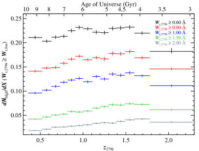
Figure 6.— Mg II absorber line density evolution. The number of absorbers per co-moving path length increases from $z_{2796}=0.4\rightarrow\ \approx\!1.6$. As expected from the flattening of $f(W_{\rm r})$ towards higher redshift (Figure 4), the stronger systems show more evolution, increasing in number towards higher redshift. We are typically 50% complete at $W_{\rm r}\approx 0.8\,\mbox{\AA}$.

$\begin{array}[]{cc}\includegraphics[width=212.47617pt]{fig7a.pdf}&\includegraphics[width=212.47617pt]{fig7b.pdf}\end{array}$

Figure 7.— Redshift (left) and co-moving path length (right) Mg II line densities. We compare apples-to-apples $d\mathcal{N}_{\mathrm{Mg\,II}}/dz$ with $W_{\rm r}\geq 1\,\mbox{\AA}$ from six surveys: this work (blue plusses); N05 (cyan crosses); P06 (light gray squares); Prochter et al. (2006b, dark gray squares); ZM13 (green diamonds); and Matejek & Simcoe (2012, red triangles). The redshift density steadily increases from $z\approx 0.4$ to $\approx 1.75$. The relatively flat $d\mathcal{N}_{\mathrm{Mg\,II}}/dX$ indicates modest evolution in the product of the co-moving number density and the physical cross-section of the absorbing clouds.

3.3. Comparing with Previous SDSS Mg II Results

Previous SDSS Mg II surveys typically fitted $f(W_{\rm r}{}_{,\mathrm{2796}})$ with an exponential model and measure $d\mathcal{N}_{\mathrm{Mg\,II}}/dz$ as a function of redshift, and here we compare their results with ours. The biggest caveat when comparing results is: all SDSS Mg II studies are statistically correlated, since they are based on subsets of the same observations. In addition, there are dependencies between methodologies. Since ZM13 used Q11 as a training set, and the latter, in turn, was based heavily on the methodologies of N05, the results of these studies are highly correlated.

All studies that fitted $f(W_{\rm r})$ (; ) find it well-modeled by an exponential, with no apparent break over $0.3\,\mbox{\AA}\lesssim W_{\rm r}{}_{,\mathrm{2796}}\lesssim 10\,\mbox{\AA}$. These studies fitted the frequency distribution as: $f(W_{\rm r})=d\mathcal{N}_{\mathrm{Mg\,II}}/dW_{\rm r}/dz=\mathcal{N}^{\ast}/W^{\ast}\exp(-W_{\rm r}/W^{\ast})$, which relates better to a Schechter function formalism. Relating our fit parameters to this formalism yields: $k=-\mathcal{N}^{\ast}\alpha$ and $\alpha=-(W^{\ast})^{-1}$. N05 found that the characteristic equivalent width, $W^{\ast}$, increased steadily in their three redshift bins covering $z=0.4\rightarrow 2.3$. Over their 12 redshift bins, ZM13 measured a turnover in $W^{\ast}$ at $z\approx 1.75$. Matejek & Simcoe (2012) measured a monotonically decreasing $W^{\ast}$ from $z=2\rightarrow 5.5$, which mapped well on to the N05 values.

For comparison, we fit the frequency distribution in redshift space and convert the best-fit parameters, $k$ and $\alpha$, to the fairly comparable quantities, $\mathcal{N}^{\ast}$ and $W^{\ast}$. We measure steadily increasing $W^{\ast}$ with redshift, in agreement with N05. N05 detect no evolution in $\mathcal{N}^{\ast}$ over $z=0.4$ to 2.3 (three redshift bins). Matejek & Simcoe (2012) also detect no evolution from $z=2$ to 5.5 (also three bins). However, the Matejek & Simcoe values are about 50% larger than the N05 measurements, with no obvious evolution in the total of six redshift bins to bring this about. On the other hand, $\mathcal{N}^{\ast}$ as estimated by ZM13 steadily increases from $z=0.4$ to 2.3, mapping well on to the high-redshift values.

However, as shown in Figure 5, the fit parameters are correlated: small increases in $W^{\ast}$ (or decreases in $\alpha$) decreases $\mathcal{N}^{\ast}$ (increases $k$). The measured $d\mathcal{N}_{\mathrm{Mg\,II}}/dz$, which is a well-measured quantity, basically defines the error ellipse. Therefore, though N05 and our $W^{\ast}$ values evolve consistently on to the high-redshift measurements, both our $\mathcal{N}^{\ast}$ values disagree with the high-redshift estimates. For us, this manifests as a turnover in $\mathcal{N}^{\ast}$ at $z\approx 1.5$, while the ZM13 values steadily increase.

We compare our $W_{\rm r}{}_{,\mathrm{2796}}\geq 1\,\mbox{\AA}$ $d\mathcal{N}_{\mathrm{Mg\,II}}/dz$ and $d\mathcal{N}_{\mathrm{Mg\,II}}/dX$ values to the other studies in Figure 7. We compiled $d\mathcal{N}_{\mathrm{Mg\,II}}/dz$ from the literature as follows: N05—Figure 9; Prochter et al. (2006b)—best-fit polynomial, updating P06; ZM13—Figure 13; and Matejek & Simcoe (2012)—Table 5. As for $d\mathcal{N}_{\mathrm{Mg\,II}}/dX$, we use: P06—Table 3 and Matejek & Simcoe (2012)—Table 5. As needed, we convert one line density to the other using $dz/dX$ or its inverse, computed at the appropriate redshift.

For all studies, the redshift density steadily increases from $z\approx 0.4$ to at least $z\approx 1.8$, and comparing to the high-redshift values (Matejek & Simcoe, 2012), there appears to be a peak between $z\approx 1.5$ and 3.

However, expansion of the universe contributes to the evolution of $d\mathcal{N}_{\mathrm{Mg\,II}}/dz$. Thus, we turn to $d\mathcal{N}_{\mathrm{Mg\,II}}/dX$, where the normalization by co-moving path length removes the effect of passive evolution. In Figure 7, $d\mathcal{N}_{\mathrm{Mg\,II}}/dX$ evolves less strongly. Examining just the SDSS results, the peak appears to be between $z\approx 1.5$ and 2. The $z=2$ to 3 values from Matejek & Simcoe (2012) are larger than the highest-redshift SDSS values but consistent within the large uncertainties.

Now we discuss why the SDSS $d\mathcal{N}_{\mathrm{Mg\,II}}/dX$ measurements, which are drawn from the same actual spectra, differ by amounts ranging from $\approx\!15\%$ (i.e., ours relative to ZM13) to $\approx\!50\%$ (relative to P06). Since the formal errors quoted by surveys ($\approx\!1\%$) are much smaller than the differences, we conclude that the uncertainties are dominated by systematic effects explored below, in addition to completeness corrections, which are not discussed. Two systematic effects contribute to $d\mathcal{N}_{\mathrm{Mg\,II}}/dX$ differences: Malmquist bias and variations in $W_{\rm r}{}_{,\mathrm{2796}}$ measurements. The Malmquist bias refers to how more absorbers scatter to above $W_{\rm r}{}_{,\mathrm{lim}}$ than scatter to below, due to the $W_{\rm r}$ uncertainties, for distributions steeply rising toward weak absorbers.

Due to the exponential nature of $f(W_{\rm r})$, a small change in $W_{\rm r}{}_{,\mathrm{lim}}$ can have significant impact on the quoted $d\mathcal{N}_{\mathrm{Mg\,II}}/dX$ (see Equation 3); also, systematic differences in equivalent-width measurements affect completeness corrections, basically shifting a completeness curve to higher or lower $W_{\rm r}$. Since there is an offset in the relative equivalent-width “zero point” between studies (see Appendix A), our equivalent-width limits are effectively different and cause a shift in $d\mathcal{N}_{\mathrm{Mg\,II}}/dX$. For example, the median deviation of $W_{\rm r}{}_{,\mathrm{ZM13}}-W_{\rm r}{}_{,\mathrm{S13}}$ for matched absorbers within $\pm 1\sigma_{W}$ of $W_{\rm r}{}_{,\mathrm{2796}}=1\,\mbox{\AA}$ (where it matters most) is $\approx\!0.01\,\mbox{\AA}$ to $0.02\,\mbox{\AA}$ but with large scatter (median absolute deviation of $\approx\!0.15\,\mbox{\AA}$). If we compare our $d\mathcal{N}_{\mathrm{Mg\,II}}/dX$ values for $W_{\rm r}{}_{,\mathrm{2796}}\geq 1.1\,\mbox{\AA}$ to the ZM13 values for $W_{\rm r}{}_{,\mathrm{2796}}\geq 1\,\mbox{\AA}$ at $z<1.75$, they agree exceedingly well.

P06 had $W_{\rm r}{}_{,\mathrm{2796}}$ measurements that differed substantially from Q11, ZM13, and our values. Hence, the P06 suffer significantly from the relative $W_{\rm r}$ “zero point” issue. This effect, some unknown Malmquist bias, and, most importantly, different completeness corrections lead to P06 differing the most from our and other surveys.

Ultimately, the points of consensus for SDSS Mg II systems are: $f(W_{\rm r}{}_{,\mathrm{2796}})$ is well-modeled by an exponential; $d\mathcal{N}_{\mathrm{Mg\,II}}/dX$ peaks at $z\approx 1.5$; and the magnitude of $d\mathcal{N}_{\mathrm{Mg\,II}}/dX$ is largely consistent with the EDR results (N05), with which Lundgren et al. (2009, partial DR5) also agree.

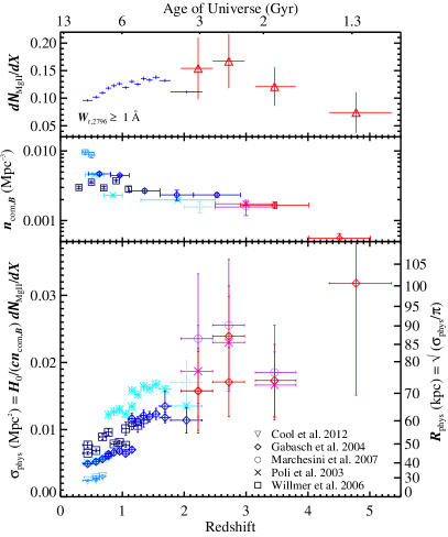
Figure 8.— Mg II-absorbing halo cross-section estimate. Assuming that all $W_{\rm r}{}_{,\mathrm{2796}}\geq 1\,\mbox{\AA}$ doublets are in B-band-selected galaxy halos (with $L\geq 0.5\,L^{\ast}$), we estimated the galaxy-Mg II cross-section as a function of $z_{2796}$ (Equation 6). Top: We used $d\mathcal{N}_{\mathrm{Mg\,II}}/dX$ from the current study (blue plusses) and Matejek & Simcoe (2012, red triangles). Middle: We calculated the co-moving number density of galaxies by integrating the $B$-band luminosity functions from the listed studies, down to $0.5\,L^{\ast}$. The galaxies are bright, typically star-forming galaxies, known to be associated with $z\lesssim 2$ Mg II absorbers (e.g., Martin & Bouché, 2009; Rubin et al., 2013). Bottom: The inferred cross-sections from the SDSS sample are comparable to observations (e.g., Chen et al., 2010a; Bordoloi et al., 2011; Nielsen et al., 2013). The various studies providing the luminosity function parameters are linked by symbol across redshift and by color between the middle and bottom panels. If possible, we show multiple $n_{{\rm com,}B}$ and $\sigma_{\rm phys}$ per redshift, because the scatter between different studies characterizes the uncertainty in $\sigma_{\rm phys}$ better than the estimated errors of any one survey.

4. Discussion

Our Mg II catalog, in conjunction with the high-redshift survey of Matejek & Simcoe (2012), traces the cosmic chemical enrichment cycle from $z_{2796}=0.4\rightarrow 5.5$, or from 10 Gyr to 1 Gyr after the Big Bang. Here we examine how the evolution in $d\mathcal{N}_{\mathrm{Mg\,II}}/dX$ relates to galaxy evolution and how various absorber populations evolve.

4.1. Mg II Evolution

Considering the direct evidence for strong Mg II systems arising in the gaseous halos of galaxies (e.g., Chen et al., 2010a; Churchill et al., 2013), especially star-forming ones (e.g., Martin & Bouché, 2009; Rubin et al., 2013), we estimate the physical cross-section of Mg II absorbers, $\sigma_{\rm phys}$, by assuming the co-moving number density of clouds equals $n_{{\rm com,}B}$, the co-moving number density of $B$-band-selected galaxies, i.e.,:

$$\frac{\displaystyle d\mathcal{N}_{\mathrm{Mg\,II}}}{\displaystyle dX}=\frac{\displaystyle c}{\displaystyle H_{0}}n_{{\rm com,}B}\sigma_{\rm phys}{\rm.}$$ (6)

These galaxies are bright, typically star-forming galaxies, known to be associated with $z\lesssim 2$ Mg II absorbers (e.g., Martin & Bouché, 2009; Rubin et al., 2013).

In Figure 8, we calculate $n_{{\rm com,}B}$ by integrating the $B$-band luminosity functions from Poli et al. (2003, crosses), Gabasch et al. (2004, diamonds), Willmer et al. (2006, squares), Marchesini et al. (2007, circles), and Cool et al. (2012, inverted triangles), down to $0.5\,L^{\ast}$. At $z_{2796}<2.3$, where the cross-section uncertainties are dominated by the $n_{{\rm com,}B}$ errors, $\sigma_{\rm phys}\ \approx 0.005\,\mathrm{Mpc}^{2}$ to $0.015\,\mathrm{Mpc}^{2}$. Assuming the Mg II-absorbing gas is distributed uniformly in a projected disk on the sky, the radius would be 40$\,\mathrm{kpc}$ to 70$\,\mathrm{kpc}$ (right-hand axis) for the SDSS redshift range, which agrees well with the observed radial profile of Mg II-absorbing galaxy halos (Chen et al., 2010a; Bordoloi et al., 2011; Nielsen et al., 2013, though see Werk et al. 2013) and permits variation in the luminosity limit and/or covering fraction. The cross-section is larger at higher redshifts, suggesting that $L<0.5\,L^{\ast}$ galaxies may contribute.

However, ultra-strong ($W_{\rm r}\geq 3\,\mbox{\AA}$) Mg II systems might be associated with galaxy group gas (Gauthier, 2013). If we limit $d\mathcal{N}_{\mathrm{Mg\,II}}/dX$ to $1\,\mbox{\AA}\leq W_{\rm r}<3\,\mbox{\AA}$ systems, the cross-sections is reduced by $5\%$ to $10\%$ from $z=0.4$ to 2.3. Recent work by Werk et al. (2013) on the CGM of $z\approx 0.2$, $L^{\ast}$ galaxies showed that the covering fraction for $W_{\rm r}{}_{,\mathrm{2796}}\geq 1\,\mbox{\AA}$ is small ($\lesssim 30\%$ within 50$\,\mathrm{kpc}$). It is difficult to compare the SDSS systems with those of Werk et al. (2013) because they have small statistics on the $W_{\rm r}\geq 1\,\mbox{\AA}$ absorbers.

Chen et al. (2010b) find a tighter correlation between $W_{\rm r}{}_{,\mathrm{2796}}$ and the projected distance to the host galaxy if the latter is scaled by the $B$-band luminosity: $R_{\rm gas}=75\times(L_{B}/L^{\ast})^{0.35}\,h^{-1}\,\mathrm{kpc}$. If we adopt this model, we can estimate the limiting luminosity, $L_{\rm lim}$, across redshift that best reproduces the observed $d\mathcal{N}_{\mathrm{Mg\,II}}/dX$. Roughly, $L_{\rm lim}\approx 0.015\,L^{\ast}$ at $z_{2796}=0.4$ and increases to $\approx 0.1\,L^{\ast}$ at $z_{2796}=1.8$ before dropping slightly in the last SDSS redshift bin. This would increase $n_{{\rm com,}B}$ by up to a factor of two, but both $n_{{\rm com,}B}$ and an estimated $\sigma_{\rm phys}$ would evolve roughly as shown. The big caveat to applying the Chen et al. (2010b) relation is that it was calibrated at $z_{2796}<0.5$, for $W_{\rm r}{}_{,\mathrm{2796}}\lesssim 3\,\mbox{\AA}$, and with $L\gtrsim 0.1\,L^{\ast}$ galaxies.

In Paper I, the C IV-absorbing cross-section was estimated to be roughly constant from $z_{1548}\approx 1.5\rightarrow 4.5$, assuming the co-moving density of clouds equals that of UV-selected galaxies, and the evolution of $n_{\rm com,UV}$ drives the approximately two-fold decrease of $d\mathcal{N}_{\rm C\,IV}/dX$ in the redshift interval. In comparison, evolution in $d\mathcal{N}_{\mathrm{Mg\,II}}/dX$ might be driven by the (large) increase in the Mg II-absorbing cross-section of galaxies from low-to-high redshift (Figure 8). Though, the evolution might be a result of a changing population of galaxies (e.g., $L<0.5\,L^{\ast}$) that host Mg II absorbers. We will explore these scenarios in a future paper.

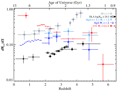
Figure 9.— Line density evolution of various absorber populations: $\tau>2$ H I systems (i.e., LLS and DLA; gray); DLAs only (black); strong Mg II and C IV systems (blue and red, respectively); and weaker Mg II systems at high redshift (cyan) from the following studies: H I—Fumagalli et al. (2013, circles); DLA—Rao et al. (2006, diamonds), Prochaska & Wolfe (2009, filled squares), Noterdaeme et al. (2012, squares); Mg II—current work (plusses), Matejek & Simcoe (2012, triangles); and C IV—Cooksey et al. (2010, filled circle), Paper I (plusses), Simcoe et al. (2011, crosses).

4.2. Evolution of Various Absorber Populations

Most, if not all, SDSS Mg II systems have other metal lines and, where coverage exists, H I absorption. These associated transitions assisted our visual verification, and in their automated procedure, ZM13 used detection of (probable) Fe II lines to disentangle Mg II doublets from other possible identifications. In addition to transitions of H I Lyman series and iron, Mg II systems can have aluminium, silicon, and/or carbon absorption. Here we examine $d\mathcal{N}_{\rm ion}/dX$ of various samples, selected on the basis of different transitions—DLAs, Lyman-limit systems (LLSs), strong C IV, and strong and weaker Mg II—and discuss the evolution of these common tracers of the CGM and IGM across cosmic time (Figure 9).

The differently evolving absorbers in Figure 9 could be physically explained, independently, as follows: (i) optical depth $\tau\geq 2$ H I systems decrease with time as the universe becomes more ionized; (ii) strong C IV systems increase with the increasing metallicity of the universe; (iii) strong Mg II systems evolve with time in lock-step with $\rho_{\ast}$; and (iv) weaker Mg II systems are established early or constantly replenished so as to evolve little. Though these explanations may be partially or completely true, they neither consider nor shed light on the evolution of the other ions. We attempt to describe the evolution of common QAL systems holistically.

We postulate that each ion has multiple sub-populations, which together, yield the observed $d\mathcal{N}_{\rm ion}/dX$. A difficulty arises in how to fairly compare the data, considering the varying equivalent-width, column-density, or optical-depth limits. For this discussion, we simply compile the best published values for a given cutoff. For $\tau\geq 2$ H I systems (i.e., LLSs and DLAs), we use the compilation by Fumagalli et al. (2013), which is based on their measurement at $z=2.8$ and Ribaudo et al. (2011, values centered at $z<1.5$), O’Meara et al. (2013, $1.5<z<3$), and Prochaska et al. (2010, $z>3.5$). The DLA-only $d\mathcal{N}/dX$ values are from Rao et al. (2006, $z<2$), Noterdaeme et al. (2012, $2<z<3.5$), and Prochaska & Wolfe (2009, $2<z<5.5$). The current work and Matejek & Simcoe (2012, $z>2$) provide $d\mathcal{N}_{\mathrm{Mg\,II}}/dX$ for $W_{\rm r}{}_{,\mathrm{2796}}\geq 1\,\mbox{\AA}$, and the line densities for $0.3\,\mbox{\AA}\leq W_{\rm r}{}_{,\mathrm{2796}}<1\,\mbox{\AA}$ absorbers are from the latter survey. For $W_{\rm r}{}_{,\mathrm{1548}}\geq 0.6\,\mbox{\AA}$ C IV systems, we use Cooksey et al. (2010, $z<1$), Paper I ($1.5<z<4.5$), and Simcoe et al. (2011, $z>4.5$).

In the original SDSS Mg II paper, N05 discussed “multiple Mg II” populations. They noted that DLAs, possible disks of star-forming galaxies, are a fraction of strong Mg II systems and that bright, spiral galaxies are not guaranteed to be found near all strong Mg II absorbers, statistically. Rao et al. (2006) estimated that $\approx\!35\%$–40% of Mg II systems with $W_{\rm r}{}_{,\mathrm{2796}}\geq 0.5\,\mbox{\AA}$ and a few other constraints (Fe II $\lambda 2600$ and Mg I $\lambda 2852$ absorption, doublet ratio) were DLAs at $z<1.65$.

The fraction of $W_{\rm r}{}_{,\mathrm{2796}}\geq 1\,\mbox{\AA}$ Mg II systems exhibiting dampled $\mathrm{Ly}\alpha$ absorption is consistent with the observed $\approx\!35\%$–40%, over the same redshift range. Overall, the fraction grows from low-to-high redshift, becoming greater than unity at $z\approx 4$, but the ratio of DLAs to $0.3\,\mbox{\AA}\leq W_{\rm r}{}_{,\mathrm{2796}}<1\,\mbox{\AA}$ Mg II systems, though also growing, stays below 100%. Matejek & Simcoe (2012) and ZM13 show that $d\mathcal{N}_{\mathrm{Mg\,II}}/dX$ for these weaker systems is roughly constant from $z=0.4\rightarrow 5.5$. Thus, the equivalent-width limit of the DLA-tracing Mg II population may evolve with redshift.

Churchill et al. (2000) proposed a Mg II taxonomy: Classic, Single/Weak, C IV-Deficient, Double, and DLA/H I-rich. They identified these classes from non-parametric clustering analysis of 30 Mg II systems with measured equivalent widths of $\mathrm{Ly}\alpha$, Mg II, Fe II (or limits), and C IV (or limits). Their sample came from 45 $0.4<z<1.4$ Mg II systems with high-resolution optical and low-resolution UV spectroscopy and had $W_{\rm r}{}_{,\mathrm{2796}}<1.8\,\mbox{\AA}$, and $W_{\rm r}{}_{,\mathrm{1548}}<2\,\mbox{\AA}$. The Classic and Double Mg II absorbers—30% and 10%, respectively, of the 30—are C IV strong, with the latter having the largest $W_{\rm r}{}_{,\mathrm{1548}}$ and $W_{\rm r}{}_{,\mathrm{2796}}$, possibly because they are two, close Classic systems. Single/Weak systems (23%) are C IV-weak but not remiss of absorption like the C IV-Deficient group (20%). The DLA/H I-rich class comprise the remaining 17% and have the largest $W_{\rm r}{}_{,\mathrm{2796}}$ but $W_{\rm r}{}_{,\mathrm{1548}}$ is comparable to the Single/Weak population.

The fraction of strong Mg II systems, not in DLAs, relative to C IV systems grows from $\approx\!10\%$ at low redshift to roughly 40% at $z\approx 3$, before decreasing sharply. For the overlapping redshift range, this is consistent with the Churchill et al. (2000) sample, if they were to define a “strong Mg II and C IV but not DLA” class. The steep $z>3$ decline is due to non-DLA, strong Mg II systems vanishing, possibly, as the weaker Mg II systems encompass a significant DLA population.

However, the ratio of non-DLA Mg II absorbers to non-DLA H I systems (i.e., LLSs) roughly decreases from $\approx\!50\%$ at $z=1$ to zero at $z=4$, though the rate of decline is steeper at $z\gtrsim 2$ to 3. The steeper decline could be due to there being less strong Mg II systems after the $\rho_{\ast}$ peak, as discussed previously, or because there is an increasing LLS sub-population due to the (metal-poor) IGM at high redshift (Fumagalli et al., 2013).

We are not able to disentangle a C IV-Deficient, (strong) Mg II population at any redshift because $d\mathcal{N}_{\rm C\,IV}/dX$ ($W_{\rm r}{}_{,\mathrm{1548}}\geq 0.6\,\mbox{\AA}$) is larger than $d\mathcal{N}_{\mathrm{Mg\,II}}/dX$ ($W_{\rm r}{}_{,\mathrm{2796}}\geq 1\,\mbox{\AA}$) at all redshifts. However, in the Churchill et al. (2000) sample, one-half to one-third of the Single/Weak class have SDSS-strength C IV absorption, which is roughly 10% of their entire sample. The shape of the C IV $f(W_{\rm r})$ does not evolve significantly over $z=1.5\rightarrow 4.5$ (Paper I); instead, the overall normalization changes smoothly, driving the evolution in $d\mathcal{N}_{\rm C\,IV}/dX$. Thus, the sub-populations comprising the $W_{\rm r}{}_{,\mathrm{1548}}\geq 0.6\,\mbox{\AA}$ systems must evolve smoothly or “conspiratorially” to preserve the shape of $f(W_{\rm r}{}_{,\mathrm{1548}})$.

Fundamentally, the number of observed systems and their associated ions are determined by: elemental abundances; strength and shape of the ionizing radiation; and the spatial distribution (e.g., density, cross-section) of the gas. The complex physics involved make cosmological simulations, if they resolve enrichment processes in the CGM and IGM, a powerful tool in understanding the evolution of various absorber populations in tandem. On the flip side, results from QAL studies are top-level constraints on ongoing and cumulative enrichment processes and should be leveraged to assess whether cosmological simulations reproduce reality. From the observational plane, we will revisit the issue of the evolution of various absorber populations in a future paper.

5. Summary

We have conducted a survey for Mg II systems in 79,294 SDSS DR7 quasar spectra (Schneider et al., 2010); these were chosen because they were not BAL QSOs and had median $\langle{\rm S/N}\rangle\geq 4\,{\rm pixel}^{-1}$ in the region covering intergalactic Mg II absorption. Candidate Mg II doublets were automatically detected, and the final catalog was visually verified. This resulted in 34,254 doublets with $\delta v_{\rm QSO}<-5000\,{\rm km\,s}^{-1}$ and outside the quasar C IV emission region, used for further analyses; the full catalog and other tools for analysis (e.g., completeness grids) are made available for the community. Our Monte-Carlo completeness tests included the effects of the automated algorithms and user bias (e.g., the accepted false-positive rate).

Though there exist differences in methodologies, from continuum fitting to final doublet selection, we recovered over 76% of the P06 absorbers, 80% of Q11, and 72% of ZM13. We also detect systems not in these other SDSS catalogs.

We analyzed the catalog as a whole and in 14 small redshift bins with roughly 2500 doublets each. The equivalent-width frequency distribution is described well by an exponential model for all redshifts. It flattens with increasing redshift, indicating there are more strong absorbers relative to weaker ones. Moreover, the best-fit parameters evolve relatively smoothly from low-to-intermediate redshift.

We compare $d\mathcal{N}_{\mathrm{Mg\,II}}/dX$ for a range of limiting equivalent widths and find significant differential evolution with $W_{\rm r}{}_{,\mathrm{lim}}$. Namely, the stronger Mg II systems evolve more with redshift, as predicted by the changing shape of $f(W_{\rm r})$ over time. In addition, the peak in $d\mathcal{N}_{\mathrm{Mg\,II}}/dX$ appears to be at higher redshift for larger $W_{\rm r}{}_{,\mathrm{lim}}$.

All SDSS studies detect the $d\mathcal{N}_{\mathrm{Mg\,II}}/dz$ increase and a peak between $z\approx 1.5$ to 2.3. On the other hand, we do not measure a decrease in the characteristic equivalent width, $W^{\ast}$, at $z_{2796}>1.75$ seen in ZM13. However, it is difficult to disentangle the degeneracy between $W^{\ast}$ and $\mathcal{N}^{\ast}$ (i.e., $\alpha$ and $k$). Additionally, the $d\mathcal{N}_{\mathrm{Mg\,II}}/dX$ measurements differ by up to 50% due to differences in methodologies, and we discussed the effects of Malmquist bias and offsets in rest equivalent-width measurements. The bias arises from more absorbers scattering above $W_{\rm r}{}_{,\mathrm{lim}}$ than below, due to measurement uncertainties. A small change in in the relative $W_{\rm r}{}_{,\mathrm{2796}}$ “zero point” has a significant impact on the absorber line density. Of course, differences in completeness corrections can contribute greatly to differences in survey results.

Assuming the co-moving number density of Mg II-absorbing clouds equals the co-moving number density of $B$-band-selected galaxies with $L\geq 0.5\,L^{\ast}$, the physical cross-section of the galaxies is estimated to grow from $\sigma_{\rm phys}\approx 0.005\,\mathrm{Mpc}^{2}$ to $0.015\,\mathrm{Mpc}^{2}$ over $z=0.4\rightarrow 2.3$. The increase in $\sigma_{\rm phys}$ might drive the increase in $d\mathcal{N}_{\mathrm{Mg\,II}}/dX$, but the evolution in the line density might reflect a changing population of Mg II-absorbing galaxies. We also explored the effect of cross-section scaling with the galaxy $B$-band luminosity and with $d\mathcal{N}_{\mathrm{Mg\,II}}/dX$ for $1\,\mbox{\AA}\leq W_{\rm r}<3\,\mbox{\AA}$ systems, which are more likely individual galaxy halos as opposed to intra-group gas.

A holistic approach is taken in discussing the evolution of various absorber population, where we assume that each ion has multiple sub-populations yielding the observed $d\mathcal{N}_{\rm ion}/dX$. The intersection of DLAs and strong Mg II absorbers grows from low-to-high redshift, but weaker ($0.3\,\mbox{\AA}\leq W_{\rm r}{}_{,\mathrm{2796}}<1\,\mbox{\AA}$) Mg II systems may better trace the DLAs at $z\gtrsim 3$. The population of strong, non-DLA-tracing Mg II and strong C IV system grows from low-to-high redshift, before decreasing sharply at $z\approx 3$. Finally the fraction of non-DLA Mg II absorbers in LLSs decreases from 50% to zero over $z=1\rightarrow 4$.

This is the second paper in our Precious Metals in SDSS Quasar Spectra project. Early versions of this catalog have already been used to compare Mg II system properties across redshift (Matejek et al., 2013) and for Mg II-galaxy clustering analysis (Gauthier et al., 2013). Future Precious Metals studies include modeling Mg II-absorbing cross-sections, a fairly comparable Si IV catalog, and multi-ion classification analysis.

Appendix A Detailed Comparison with Previous SDSS Mg II Catalogs

$\begin{array}[]{ccc}\includegraphics[width=143.09538pt]{figA10a.pdf}&\includegraphics[width=143.09538pt]{figA10b.pdf}&\includegraphics[width=143.09538pt]{figA10c.pdf}\end{array}$

Figure 10.— Comparing redshift distributions of published SDSS Mg II catalogs: P06 (DR3, left); Q11 (DR4, middle); and ZM13 (DR7, right). The solid histograms show each catalog’s full distribution (for the same data release), while the dashed histograms are each catalog’s unique sample (our current catalog in black, others in red). The hard $W_{\rm r}{}_{,\mathrm{2796}}\geq 1\,\mbox{\AA}$ limit in P06 (Figure 11) drives the differences in the catalogs. For Q11 and ZM13, the systems unique to the current study tend to be at lower redshift (black, dashed histograms).

In Section 2.3, we summarized the differences between four previous Mg II surveys, that used the following SDSS data releases: early (Nestor et al., 2005); third (Prochter et al., 2006a); fourth (Quider et al., 2011); and seventh (Zhu & Ménard, 2013). Here we provide specific absorber-to-absorber details.

N05 surveyed approximately 3700 $z_{\rm QSO}\geq 0.37$ sightlines in the SDSS EDR quasar catalog (Schneider et al., 2002) and visually verified 1331 Mg II doublets with $0.3\,\mbox{\AA}\leq W_{\rm r}{}_{,\mathrm{2796}}<5.7\,\mbox{\AA}$ and $0.36<z_{2796}<2.27$. In DR7, there remains 3809 of the 3814 total QSOs in EDR, and in those, we detect 1425 absorbers with $W_{\rm r}{}_{,\mathrm{2796}}\lesssim 9\,\mbox{\AA}$ with the same redshift range. N05 did not publish their line catalog, but it was folded in to the DR4 survey of Q11, which is discussed below.

P06 surveyed 45,023 $z_{\rm QSO}>0.35$ quasar spectra in the DR3 quasar catalog (Schneider et al., 2005) and published a catalog of the resulting, visually verified 7410 doublets, with $1\,\mbox{\AA}\leq W_{\rm r}{}_{,\mathrm{2796}}\leq 10.1\,\mbox{\AA}$ and $0.36<z_{2796}\leq 2.28$. There are 44,545 DR3 sightlines in the DR7 catalog, and we identified 15,083 Mg II systems. In Figures 10 and 11, we compare $z_{2796}$ and $W_{\rm r}{}_{,\mathrm{2796}}$ for the intersection of the P06 and our catalogs (5693 doublets) and for the systems unique to either (1717 and 9390, respectively). The P06-only systems are generally spread out in redshift (Figure 10). P06 measured equivalent widths by summing the flux absorbed in 3589 Å boxes, centered at the redshift of the 2796 Å line. As can be seen in Figure 11, this and a systematically low continuum fit results in an underestimation of the equivalent width for strong systems.

We do not recover the 1717 doublets unique to P06 for the following reasons (number): in Shen et al. (2011) BAL QSO sightlines (730); $({\rm S/N})_{\rm conv}<2.5\,{\rm resel}^{-1}$ in the 2803 Å line in our normalized spectra (588); in sightlines with $\langle{\rm S/N}\rangle<4\,{\rm pixel}^{-1}$ (296); $({\rm S/N})_{\rm conv}<3.5\,{\rm resel}^{-1}$ in the 2796 Å line in our normalized spectra (65); in visual BAL QSO sightlines (35); and within 3000$\,{\rm km\,s}^{-1}$ of the Schneider et al. (2010) quasar redshift (3). Of the 9393 doublets unique to our catalog, 6787 (72%) have $W_{\rm r}{}_{,\mathrm{2796}}<1\,\mbox{\AA}$, which Prochter et al. (2006a) excluded by construction.

$\begin{array}[]{ccc}\includegraphics[trim=199.16928pt 0.0pt 0.0pt 0.0pt,width=143.09538pt]{figA11a.pdf}&\includegraphics[trim=199.16928pt 0.0pt 0.0pt 0.0pt,width=143.09538pt]{figA11b.pdf}&\includegraphics[trim=199.16928pt 0.0pt 0.0pt 0.0pt,width=143.09538pt]{figA11c.pdf}\end{array}$

Figure 11.— Comparing rest equivalent-width distributions of published SDSS Mg II catalogs. For all catalogs, the unique systems tend to be the weaker systems (red histograms). P06 only published systems with $W_{\rm r}\geq 1\,\mbox{\AA}$ (left). They also had the largest discrepancy with our measured equivalent widths. The green, dashed lines show the one-to-one relation. The orange, dash-dot lines are linear least-squares fits, including errors in both datasets, with three-sigma errors (orange, dotted lines). The black histograms show the redshift distribution of the matched systems from each catalog.

Q11 surveyed 44,620 $z_{\rm QSO}>0.36$ quasar sightlines in the SDSS DR4 database, and they give the details of their SQL query. They visually verified 17,042 Mg II systems with $0.15\,\mbox{\AA}<W_{\rm r}{}_{,\mathrm{2796}}<6.5\,\mbox{\AA}$ and $0.36<z_{2796}<2.29$. In DR7, there remains 44,463 of the DR4 quasars, in which we detect 18,188 systems. The intersection of our catalogs yields 13,783 systems, leaving 3258 doublets unique to Q11 and 4405 to us; Figures 10, 11, and 12 show the $z_{2796}$, $W_{\rm r}{}_{,\mathrm{2796}}$, and $W_{\rm r}{}_{,\mathrm{2796}}$/$W_{\rm r}{}_{,\mathrm{2803}}$ distributions for matched and unique samples. There is an excess of our unique Mg II systems, at low redshift. Our $W_{\rm r}{}_{,\mathrm{2796}}$ measurements agreed well, even though Q11 used Gaussian fits and we used boxcar summation, and systems unique to either catalog tend to cluster at $W_{\rm r}{}_{,\mathrm{2796}}<1\,\mbox{\AA}$. There is a significant tilt when comparing our equivalent-width ratios, and our unique systems tend to have ratios less than unity, which mean they have blended 2803 Å lines.

We do not recover 3260 systems unique to Q11 for the following reasons (number): in BAL QSO sightlines (1617); $({\rm S/N})_{\rm conv}<2.5\,{\rm resel}^{-1}$ in the 2803 Å line (1172) and $({\rm S/N})_{\rm conv}<3.5\,{\rm resel}^{-1}$ in the 2796 Å line (294) in our normalized spectra; in visual BAL QSO sightlines (94); in sightlines with $\langle{\rm S/N}\rangle<4\,{\rm pixel}^{-1}$ (79); and in sightlines no longer in DR7 (4). Of the 4403 doublets unique to our catalog, 3092 (70%) have $W_{\rm r}{}_{,\mathrm{2796}}<1\,\mbox{\AA}$.

ZM13 surveyed a total of 84,533 DR7 quasar spectra, 569 from Hewett & Wild (2010) and the rest from Schneider et al. (2010). For all quasars, ZM13 adopted the Hewett & Wild (2010) quasar redshifts. ZM13 conducted a completely automated search, using Q11 as a training set, and identified 35,752 systems with $W_{\rm r}{}_{,\mathrm{2796}}<8.5\,\mbox{\AA}$ and $0.36<z_{2796}<2.29$. Comparing our full catalog of 35,629 Mg II systems, both catalogs agree on 25,909 systems, leaving 9843 systems unique to ZM13 and 9720 to us. We show the $z_{2796}$, $W_{\rm r}{}_{,\mathrm{2796}}$, and $W_{\rm r}{}_{,\mathrm{2796}}$/$W_{\rm r}{}_{,\mathrm{2803}}$ distributions for the matched and unique samples in Figures 10, 11, and 12. There is a strong trend for our unique doublets to be at low redshift, since ZM13 did not search the C IV “forest,” requiring $\Delta z>0.02$ red-ward of the quasar C IV emission line. Our $W_{\rm r}{}_{,\mathrm{2796}}$ values agree well; ZM13 also measured the equivalent width from Gaussian fits. The doublets unique to either catalog peak at $W_{\rm r}{}_{,\mathrm{2796}}<1\,\mbox{\AA}$. There is a significant tilt in the equivalent-width-ratio plane, and our unique systems are relatively evenly distributed around a ratio of unity.

We do not recover 9843 systems unique to ZM13 for the following reasons (number): $({\rm S/N})_{\rm conv}<2.5\,{\rm resel}^{-1}$ in the 2803 Å line in our normalized spectra (5193); in BAL QSO sightlines (3075); $({\rm S/N})_{\rm conv}<3.5\,{\rm resel}^{-1}$ in the 2796 Å line in our normalized spectra (976); in sightlines with $\langle{\rm S/N}\rangle<4\,{\rm pixel}^{-1}$ (291); in visual BAL QSO sightlines (209); and in Hewett & Wild (2010) sightlines (99). Of the 9720 doublets unique to our catalog, 3387 were not recovered by ZM13 because they are in the C IV forest; 793 because they are within $\Delta z=0.04$ of the Hewett & Wild (2010) quasar Mg II emission line; and 156 because they are coincident with Galactic Ca II $\lambda\lambda 3934,3969$.

$\begin{array}[]{cc}\includegraphics[trim=199.16928pt 0.0pt 0.0pt 0.0pt,width=130.08731pt]{figA12a.pdf}&\includegraphics[trim=199.16928pt 0.0pt 0.0pt 0.0pt,width=130.08731pt]{figA12b.pdf}\end{array}$

Figure 12.— Comparing rest equivalent-width ratio distributions of published SDSS Mg II catalogs; the colored lines and histograms are similar to those described in Figure 11. (P06 did not published the equivalent widths of the Mg II 2803 Å line.) Though the equivalent widths for matched systems were largely in agreement (Figure 11), the ratios show larger disagreement (orange, dashed lines). The systems unique to Q11 and ZM13 tend to be less saturated systems (ratios $>1$; red histograms, vertical axes). Since the unique systems from all catalogs were largely lower-$W_{\rm r}{}_{,\mathrm{2796}}$ systems, it appears Q11 and ZM13 were more sensitive to weak $W_{\rm r}{}_{,\mathrm{2796}}$ doublets with weaker $W_{\rm r}{}_{,\mathrm{2803}}$ lines, while we picked up on weak, saturated and/or blended systems, where blending can drive the ratio below unity.

References

- Bergeron (1986) Bergeron, J. 1986, A&A, 155, L8
- Bordoloi et al. (2011) Bordoloi, R., et al. 2011, ApJ, 743, 10
- Bouché et al. (2012) Bouché, N., Hohensee, W., Vargas, R., Kacprzak, G. G., Martin, C. L., Cooke, J., & Churchill, C. W. 2012, MNRAS, 426, 801
- Bouché et al. (2006) Bouché, N., Murphy, M. T., Péroux, C., Csabai, I., & Wild, V. 2006, MNRAS, 371, 495
- Bouwens et al. (2010) Bouwens, R. J., et al. 2010, ApJ, 725, 1587
- Bowen & Chelouche (2011) Bowen, D. V., & Chelouche, D. 2011, ApJ, 727, 47
- Charlton et al. (2003) Charlton, J. C., Ding, J., Zonak, S. G., Churchill, C. W., Bond, N. A., & Rigby, J. R. 2003, ApJ, 589, 111
- Chen et al. (2010a) Chen, H.-W., Helsby, J. E., Gauthier, J.-R., Shectman, S. A., Thompson, I. B., & Tinker, J. L. 2010a, ApJ, 714, 1521
- Chen et al. (2010b) Chen, H.-W., Wild, V., Tinker, J. L., Gauthier, J.-R., Helsby, J. E., Shectman, S. A., & Thompson, I. B. 2010b, ApJ, 724, L176
- Churchill et al. (2000) Churchill, C. W., Mellon, R. R., Charlton, J. C., Jannuzi, B. T., Kirhakos, S., Steidel, C. C., & Schneider, D. P. 2000, ApJ, 543, 577
- Churchill et al. (2013) Churchill, C. W., Nielsen, N. M., Kacprzak, G. G., & Trujillo-Gomez, S. 2013, ApJ, 763, L42
- Churchill et al. (1999) Churchill, C. W., Rigby, J. R., Charlton, J. C., & Vogt, S. S. 1999, ApJS, 120, 51
- Cooksey et al. (2013) Cooksey, K. L., Kao, M. M., Simcoe, R. A., O’Meara, J. M., & Prochaska, J. X. 2013, ApJ, 763, 37
- Cooksey et al. (2010) Cooksey, K. L., Thom, C., Prochaska, J. X., & Chen, H. 2010, ApJ, 708, 868
- Cool et al. (2012) Cool, R. J., et al. 2012, ApJ, 748, 10
- Cucchiara et al. (2013) Cucchiara, A., et al. 2013, ApJ, 773, 82
- Fumagalli et al. (2013) Fumagalli, M., O’Meara, J. M., Prochaska, J. X., & Worseck, G. 2013, ApJ, 775, 78
- Gabasch et al. (2004) Gabasch, A., et al. 2004, A&A, 421, 41
- Gauthier (2013) Gauthier, J.-R. 2013, MNRAS, 432, 1444
- Gauthier & Chen (2011) Gauthier, J.-R., & Chen, H.-W. 2011, MNRAS, 418, 2730
- Gauthier et al. (2013) Gauthier, J.-R., Chen, H.-W., Cooksey, K. L., Simcoe, R. A., Seyffert, E. N., & O’Meara, J. M. 2013, ArXiv e-prints
- Gauthier et al. (2010) Gauthier, J.-R., Chen, H.-W., & Tinker, J. L. 2010, ApJ, 716, 1263
- Hewett & Wild (2010) Hewett, P. C., & Wild, V. 2010, MNRAS, 405, 2302
- Kacprzak et al. (2011a) Kacprzak, G. G., Churchill, C. W., Barton, E. J., & Cooke, J. 2011a, ApJ, 733, 105
- Kacprzak et al. (2011b) Kacprzak, G. G., Churchill, C. W., Evans, J. L., Murphy, M. T., & Steidel, C. C. 2011b, MNRAS, 416, 3118
- Kacprzak et al. (2012) Kacprzak, G. G., Churchill, C. W., & Nielsen, N. M. 2012, ApJ, 760, L7
- Komatsu et al. (2009) Komatsu, E., et al. 2009, ApJS, 180, 330
- Kornei et al. (2012) Kornei, K. A., Shapley, A. E., Martin, C. L., Coil, A. L., Lotz, J. M., Schiminovich, D., Bundy, K., & Noeske, K. G. 2012, ApJ, 758, 135
- Lanzetta et al. (1987) Lanzetta, K. M., Turnshek, D. A., & Wolfe, A. M. 1987, ApJ, 322, 739
- Lovegrove & Simcoe (2011) Lovegrove, E., & Simcoe, R. A. 2011, ApJ, 740, 30
- Lundgren et al. (2009) Lundgren, B. F., et al. 2009, ApJ, 698, 819
- Marchesini et al. (2007) Marchesini, D., et al. 2007, ApJ, 656, 42
- Martin & Bouché (2009) Martin, C. L., & Bouché, N. 2009, ApJ, 703, 1394
- Matejek & Simcoe (2012) Matejek, M. S., & Simcoe, R. A. 2012, ApJ, 761, 112
- Matejek et al. (2013) Matejek, M. S., Simcoe, R. A., Cooksey, K. L., & Seyffert, E. N. 2013, ApJ, 764, 9
- Ménard et al. (2011) Ménard, B., Wild, V., Nestor, D., Quider, A., Zibetti, S., Rao, S., & Turnshek, D. 2011, MNRAS, 417, 801
- Misawa et al. (2008) Misawa, T., Charlton, J. C., & Narayanan, A. 2008, ApJ, 679, 220
- Narayanan et al. (2007) Narayanan, A., Misawa, T., Charlton, J. C., & Kim, T.-S. 2007, ApJ, 660, 1093
- Nestor et al. (2011) Nestor, D. B., Johnson, B. D., Wild, V., Ménard, B., Turnshek, D. A., Rao, S., & Pettini, M. 2011, MNRAS, 412, 1559
- Nestor et al. (2005) Nestor, D. B., Turnshek, D. A., & Rao, S. M. 2005, ApJ, 628, 637
- Nielsen et al. (2013) Nielsen, N. M., Churchill, C. W., Kacprzak, G. G., & Murphy, M. T. 2013, ApJ, 776, 114
- Noterdaeme et al. (2012) Noterdaeme, P., et al. 2012, A&A, 547, L1
- O’Meara et al. (2013) O’Meara, J. M., Prochaska, J. X., Worseck, G., Chen, H.-W., & Madau, P. 2013, ApJ, 765, 137
- Petitjean & Bergeron (1990) Petitjean, P., & Bergeron, J. 1990, A&A, 231, 309
- Poli et al. (2003) Poli, F., et al. 2003, ApJ, 593, L1
- Prochaska et al. (2010) Prochaska, J. X., O’Meara, J. M., & Worseck, G. 2010, ApJ, 718, 392
- Prochaska & Wolfe (2009) Prochaska, J. X., & Wolfe, A. M. 2009, ApJ, 696, 1543
- Prochter et al. (2006a) Prochter, G. E., Prochaska, J. X., & Burles, S. M. 2006a, ApJ, 639, 766
- Prochter et al. (2006b) Prochter, G. E., et al. 2006b, ApJ, 648, L93
- Quider et al. (2011) Quider, A. M., Nestor, D. B., Turnshek, D. A., Rao, S. M., Monier, E. M., Weyant, A. N., & Busche, J. R. 2011, AJ, 141, 137
- Rao & Turnshek (2000) Rao, S. M., & Turnshek, D. A. 2000, ApJS, 130, 1
- Rao et al. (2006) Rao, S. M., Turnshek, D. A., & Nestor, D. B. 2006, ApJ, 636, 610
- Ribaudo et al. (2011) Ribaudo, J., Lehner, N., & Howk, J. C. 2011, ApJ, 736, 42
- Rigby et al. (2002) Rigby, J. R., Charlton, J. C., & Churchill, C. W. 2002, ApJ, 565, 743
- Rubin et al. (2013) Rubin, K. H. R., Prochaska, J. X., Koo, D. C., Phillips, A. C., Martin, C. L., & Winstrom, L. O. 2013, ArXiv e-prints
- Rubin et al. (2010) Rubin, K. H. R., Weiner, B. J., Koo, D. C., Martin, C. L., Prochaska, J. X., Coil, A. L., & Newman, J. A. 2010, ApJ, 719, 1503
- Sargent et al. (1988) Sargent, W. L. W., Steidel, C. C., & Boksenberg, A. 1988, ApJ, 334, 22
- Schneider et al. (2005) Schneider, D. P., et al. 2005, AJ, 130, 367
- Schneider et al. (2002) —. 2002, AJ, 123, 567
- Schneider et al. (2010) —. 2010, AJ, 139, 2360
- Shen et al. (2011) Shen, Y., et al. 2011, ApJS, 194, 45
- Simcoe et al. (2011) Simcoe, R. A., et al. 2011, ApJ, 743, 21
- Steidel & Sargent (1992) Steidel, C. C., & Sargent, W. L. W. 1992, ApJS, 80, 1
- Weiner et al. (2009) Weiner, B. J., et al. 2009, ApJ, 692, 187
- Werk et al. (2013) Werk, J. K., Prochaska, J. X., Thom, C., Tumlinson, J., Tripp, T. M., O’Meara, J. M., & Peeples, M. S. 2013, ApJS, 204, 17
- Willmer et al. (2006) Willmer, C. N. A., et al. 2006, ApJ, 647, 853
- Wolfe et al. (2005) Wolfe, A. M., Gawiser, E., & Prochaska, J. X. 2005, ARA&A, 43, 861
- York et al. (2000) York, D. G., et al. 2000, AJ, 120, 1579
- Zhu & Ménard (2013) Zhu, G., & Ménard, B. 2013, ApJ, 770, 130