Non-isothermal filaments in equilibrium

Abstract

Context. The physical properties of the so-called Ostriker isothermal filament (Ostriker 1964) have been classically used as benchmark to interpret the stability of the filaments observed in nearby clouds. However, recent continuum studies have shown that the internal structure of the filaments depart from the isothermality, typically exhibiting radially increasing temperature gradients.

Aims. The presence of internal temperature gradients within filaments suggests that the equilibrium configuration of these objects should be therefore revisited. The main goal of this work is to theoretically explore how the equilibrium structure of a filament changes in a non-isothermal configuration.

Methods. We solve the hydrostatic equilibrium equation assuming temperature gradients similar to those derived from observations.

Results. We obtain a new set of equilibrium solutions for non-isothermal filaments with both linear and asymptotically constant temperature gradients. Our results show that, for sufficiently large internal temperature gradients, a non-isothermal filament could present significantly larger masses per unit length and shallower density profiles than the isothermal filament without collapsing by its own gravity.

Conclusions. We conclude that filaments can reach an equilibrium configuration under non-isothermal conditions. Detailed studies of both the internal mass distribution and temperature gradients within filaments are then needed in order to judge the physical state of filaments.

1 Introduction

Although the observations of filaments within molecular clouds have been reported since decades (e.g. Schneider & Elmegreen, 1979), only recently their presence has been recognized as a unique characteristic of the star-formation process. The latest Herschel results have revealed the direct connection between the filaments, dense cores and stars in all kinds of environments along the Milky Way, from low-mass and nearby clouds (André et al., 2010) to most distant and high-mass star-forming regions (Molinari et al., 2010). As a consequence, characterizing the physical properties of these filaments has been revealed as key to our understanding of the origin of the stars within molecular clouds.

Classically, filaments have been interpreted assuming that $(i)$ they are isothermal, $(ii)$ they are isolated, $(iii)$ they can be modeled as cylindrical structures with infinite length, and $(iv)$ that their support against gravity comes solely from thermal pressure. However, observational evidence is mounting that none of the above hypotheses can be considered strictly valid: $(i)$ recent continuum observations of filaments in different clouds have shown that the dust temperature gradually decreases towards the main axis of these structures (e.g. Stepnik et al., 2003; Palmeirim et al., 2013); $(ii)$ filaments are typically found forming intricate networks (e.g. hub-filament associations, Myers, 2009) or even compact bundles of small-scale filaments (Hacar et al., 2013); $(iii)$ Filaments with aspect ratios of $\sim$ 4–5 are not uncommon (Hacar & Tafalla, 2011); and $(iv)$ millimeter line studies show that the molecular emission arising from the filaments exhibit super-thermal linewidths, suggesting that the non-thermal motions could play a non-negligible role in their stability (e.g. Arzoumanian et al., 2013). The inclusion of any of these characteristics could drastically change the interpretation of the physical state of the filaments. It is then clear that the equilibrium properties of the filaments should be revisited.

In this paper we concentrate on the theoretical study of non-isothermal filaments. The main aim of this work is to show how the equilibrium structure of a filament changes if the hypothesis of isothermality is relaxed. In a companion paper (Recchi et al., in preparation) we investigate the stability and structure of non-isolated filaments. In a future paper we will investigate the effect of non-thermal pressure support within the filament.

2 Isothermal filaments

Starting from the seminal paper of Chandrasekhar & Fermi (1953), the stability of isothermal filaments has been studied by a number of authors. Stodólkiewicz (1963) and Ostriker (1964) first demonstrated that the radial profile of an isothermal filament in hydrostatic equilibrium can be described by:

$$\rho_{eq}(r)=\rho_{c}\left[1+\left(\frac{r}{H}\right)^{2}\right]^{-2},\mbox{ with }H=\sqrt{\frac{2c_{s}^{2}}{\pi G\rho_{c}}}$$ (1)

where $r$ is the radial distance from the axis, $\rho_{c}$ is the central density (i.e. the density at the axis), and $c_{s}$ is the isothermal sound speed (i.e. $c_{s}^{2}=p/\rho=kT/(\mu m_{H})$. The mass per unit length (or linear mass) of this isothermal cylinder, the so-called Ostriker filament, is given by:

$$M_{lin}\equiv M_{cr}=\int_{0}^{\infty}2\pi r\rho_{eq}(r)dr=\frac{2kT}{G\mu m_{H}}$$ (2)

Assuming a $\mu=2.3$ as a typical mean molecular weight in molecular clouds and for a temperature typical for the ISM of $T=10$ K, the linear mass of an isothermal cylinder in equilibrium is then 16.6 M_⊙ pc^-1. In filaments with larger linear masses, equilibrium between pressure and self-gravity cannot be established. Under these conditions, self-gravity prevails and the cylinder is destined to collapse into a spindle (e.g. Inutsuka & Miyama, 1992).

3 Equilibrium solutions for non-isothermal filaments

In parallel to the isothermal analysis, Ostriker (1964) also developed the theory of stability for non-isothermal cylinders. He considered a generic polytropic equation of state (EOS) $P=K_{n}\rho^{1+1/n}$ ($n$ corresponds to $1/(\gamma-1)$, where $\gamma$ is the ratio of specific heats). By combining the equation of hydrostatic equilibrium ${\nabla}P=\rho{\nabla}V$ (where $V$ is the gravitational potential) and the Poisson’s equation $\nabla^{2}V=-4\pi G\rho$, he found the equation $K_{n}(n+1)\nabla^{2}\rho^{1/n}=-4\pi G\rho$. With the change of variables $r=a\xi\equiv\left[\frac{(n+1)K_{n}}{4\pi G\rho_{c}^{1-1/n}}\right]^{1/2}\xi,\sigma=(\rho/\rho_{c})^{1/n}$ (originally defined as $\theta$ by Ostriker), the resulting equation is simply

$$\frac{d^{2}\sigma}{d\xi^{2}}+\frac{1}{\xi}\frac{d\sigma}{d\xi}=-(\sigma)^{n},$$ (3)

subject to the initial conditions $\sigma(0)=1$, $\sigma^{\prime}(0)=0$. Equation 3 has real solutions only if $n\geq-1$, or equivalently if $\gamma\geq 0$ (but see Viala & Horedt 1974 for the case $n<-1$). These solutions include the isothermal solution when $n=+\infty$ (and $\gamma=1$). Under these conditions, both the linear mass and the radius of the filament in equilibrium reach a finite value (see Ostriker 1964 for a discussion).

Nowadays, detailed observations of the dust emission in filaments offer us the unique opportunity to directly estimate their radial temperature profile (see Stepnik et al. 2003 for L1506 using PRONAOS, Nutter et al. 2008 for TMC-1 using SCUBA, and, more recently, Arzoumanian et al. 2011 for IC 5146 or Palmeirim et al. 2013 for B211 using Herschel). In contrast to the temperature profiles expected for filaments in equilibrium with polytropic EOS, the dust temperature gradients observed in nearby molecular filaments show it to be radially increasing (e.g. Stepnik et al., 2003; Palmeirim et al., 2013), probably due to the radiation field incident on the exterior of the filament complex. It is important to remark that it is impossible to obtain radially increasing temperature profiles by solving Eq. 3 for $n>-1$. In fact, $T\propto\rho^{1/n}$, hence $T\propto\sigma$. For $n>0$, both $\rho$ and $\sigma$ (hence $T$) decrease outwards. For $n=0$, corresponding to $\rho=Const$, the well-known solution is $\sigma=1-\frac{1}{4}\xi^{2}$ (decreasing outwards). It is easy to verify numerically that, for $-1<n<0$, $\sigma$ and $T$ still decrease outwards, whereas $\rho$ increases outwards because $\rho\propto\sigma^{n}$. The same result has been obtained by Viala & Horedt (1974; see their tables 11-13). It is also interesting to remark that values of $\gamma<1$ are expected for polytropic filaments in gravitational collapse, according to simulations (Kawachi & Hanawa, 1998). As a result, the observation of such temperature profiles has been interpreted as a signature of instability.

In order to take into account the observationally-based result of radially increasing temperature gradients, we must thus adopt a different approach. We assume the gas temperature profile $T(r)$ to be known and we recover the corresponding equilibrium density profile. We still use the hydrostatic equilibrium relation $\nabla P=g\rho$, reminding however that now both $T$ and $\rho$ vary with radius (we still assume $\mu$ to be constant). The resulting (integro-differential) equation is:

$$\frac{k}{\mu m_{H}}\nabla(\rho T)=\rho\cdot\left(-\frac{2G\int_{0}^{r}2\pi{\tilde{r}}\rho({\tilde{r}})d{\tilde{r}}}{r}\right),$$ (4)

Here we define $\rho=\theta\rho_{c}$, $T=\tau T_{0}$ and $r=Hx$, where $\rho_{c}$ and $T_{0}$ are the density and the temperature at the filament axis, respectively, and $H$ is given by Eq. 1, with $T=T_{0}$. The resulting normalized equation is:

$$\theta^{\prime}=-\theta\left(\frac{\tau^{\prime}}{\tau}+\frac{8}{\tau x}\int_{0}^{x}s\theta ds\right),$$ (5)

where primes indicate differentiation with respect to $x$. This equation is subject to the initial condition $\theta(0)=1$ (i.e. $\rho(x=0)=\rho_{c}$). This equation can be manipulated as follows: differentiate it with respect to $x$ and use again Eq. 5 to get rid of the integral. The resulting second-order ODE is:

$$\theta^{\prime\prime}=\frac{\left(\theta^{\prime}\right)^{2}}{\theta}-\theta^{\prime}\left(\frac{\tau^{\prime}}{\tau}+\frac{1}{x}\right)-\theta\left(\frac{\tau^{\prime\prime}}{\tau}+\frac{\tau^{\prime}}{\tau x}\right)-8\frac{\theta^{2}}{\tau},$$ (6)

where it is easy to see that the isothermal Ostriker solution, with $\theta_{i}=\left[1+x^{2}\right]^{-2}$ (i.e. the normalized version of Eq. 1), satisfies the above ODE if $\tau=1$ (i.e. $T(x)=T_{0}$). This form of the equation is more convenient than the Lane-Emden equation Eq. 3 for the problem at hand. It is also important to note that the above equation is subject to the initial conditions $\theta(0)=1$, $\theta^{\prime}(0)=-\tau^{\prime}(0)$. This initial condition is due the fact that the value of the pressure gradient at the axis must be zero (see below). The consequence of this initial condition is relevant: if the temperature profiles have positive gradients at the axis (as it appears from the observations), the density profiles must have negative gradients, i.e. they must show central cusps.

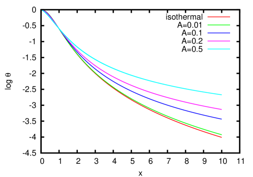
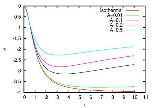
Figure 1: Normalized density profiles $\theta=\rho/\rho_{c}$ (left panel) and values of $\alpha$ (right panel; see Sect. 3.1 for the definition of $\alpha$) as a function of $x=r/H$ for models with temperature profiles described by Eq. 8, for different normalized temperature gradients $A$. The reference isothermal profile is also plotted in both panels.

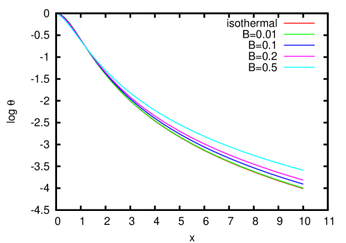
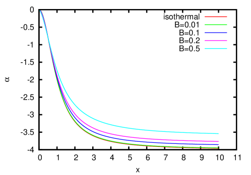
Figure 2: As Fig. 1 but for models with temperature profiles described by Eq. 10.

Another way to manipulate Eq. 4 is the following: call $\eta$ the pressure, normalized to the central value (i.e. $\eta=P/P_{0}$). The obtained integro-differential equation for $\eta$ is $\eta^{\prime}=-\frac{\eta}{x\tau}\int_{0}^{x}\frac{s\eta}{\tau}ds$. Manipulating this equation exactly as done for Eq. 5, the following differential equation can be found:

$$\eta^{\prime\prime}=\frac{\left(\eta^{\prime}\right)^{2}}{\eta}-\eta^{\prime}\cdot\left(\frac{1}{x}+\frac{\tau^{\prime}}{\tau}\right)-8\left(\frac{\eta}{\tau}\right)^{2}.$$ (7)

The initial conditions are $\eta(0)=1$ and $\eta^{\prime}(0)=0$. This second initial condition derives from the equation of hydrostatic equilibrium $\nabla P=g\rho$ if we assume $g(0)=0$. Given a temperature profile $\tau(x)$, the density profile for a non-isothermal filament in equilibrium $\theta(x)$ can be then derived solving Eqs. 6 or 7.

3.1 Filaments with linear temperature gradients

It is instructive to consider a simplified case where the temperature linearly increases with radius as:

$$\tau(x)=1+Ax,$$ (8)

where $A$ is the normalized temperature gradient in units of the normalized radius $x$. This linear increase of the temperature closely resembles the observations summarized at the beginning of this section, at least sufficiently close to the axis. We have numerically solved Eq. 6 for different values of $A$. We have also solved Eq. 7 and verified that the two solutions are identical. This is a useful check of the consistency of our solution. The resulting density profiles $\theta(x)$ are shown in Fig. 1 (left panel). We can notice from this figure that the density profile tends, as expected, to the isothermal profile $\theta_{i}=\left[1+x^{2}\right]^{-2}$ for $A\rightarrow 0$. Within the range of normalized temperature gradients considered here (i.e. $0.01\leq A\leq 0.5$), the equilibrium configuration derived from Eq. 6 closely resembles the Ostriker profile at short radii (at least sufficiently close to the axis; i.e. $x<2$). On the contrary, the derived density profiles clearly depart from the equilibrium solution for an isothermal filament at larger radii under the presence of temperature gradients with $A\geq 0.1$. Indeed, if $A=0.5$ the density profile for an non-isothermal filament in equilibrium can be more than one order of magnitude higher than the expected value in the isothermal case at $x\geq 6$.

In order to better characterize the density profile, we consider the quantity $\alpha=\frac{d\ln\theta}{d\ln x}$. If the density profile can be approximated by a power law, $\alpha$ clearly represents the exponent. The functions $\alpha(x)$ for the different density profiles discussed above as a function of the normalized radius $x$ are plotted in Fig. 1 (right panel). For the isothermal profile $\theta_{i}(x)$ it is easy to see that $\alpha=-\frac{4x^{2}}{1+x^{2}}$, with $\alpha$ tending to -4 for $x\rightarrow\infty$. Compared to the Ostriker solution, the equilibrium configuration for a non-isothermal filament with $A>0$ presents therefore shallower profiles at large radii. Particularly for $0.1\leq A\leq 0.5$, the filaments tend to present slopes with $-3\lesssim\alpha\lesssim-2$ for normalized radius within $4<x<10$.

The presence of density profiles shallower than the Ostriker solution has important implications in the linear mass that can be supported by these non-isothermal filaments. As can be seen in Fig. 1, $\alpha$ tends to increase for large values of $x$. Indeed, it is possible to show (see Appendix A) that $\alpha$ must asymptotically tend to a value $\alpha_{lim}\in]-2,-1[$. This implies also that the normalized linear mass:

$$\Pi=\int_{0}^{\infty}2\pi x\theta(x)dx,$$ (9)

diverges. This can be explained because the temperature tends to infinity for $x\rightarrow\infty$, so the increasingly large thermal pressure at large radii must be counter-balanced by an increasingly large gravity. As a consequence, the linear mass for a non-isothermal filament in equilibrium presenting a linear temperature gradient can be arbitrary large. In order to avoid the linear mass to diverge, a filament described by a temperature profile as in Eq. 8 has to be necessarily pressure-truncated at some radius.

Finally, we notice that the properties of the non-isothermal filaments derived above resemble the equilibrium configuration found in turbulent dominated filaments. Gehman et al. (1996) demonstrated that an isothermal filament with a radially increasing turbulent pressure presents a shallower density profile and larger linear mass than the equivalent Ostriker-like filament at the same temperature. Compared to the non-isothermal configuration, in these models the increasing gravitational energy is balanced by a pressure generated from the radial increase of the non-thermal motions, while in our case the filament is always thermally supported.

3.2 Filaments presenting asymptotically constant temperature gradients

It is also useful to look for a temperature profile resembling Eq. 8 for small values of $x$ but tending to a finite value for $x\rightarrow\infty$. These kinds of profiles are similar to those found in the observations where the temperature flattens out for large radii (typically at radii $\sim$ 0.4-0.5 pc; see e.g. Stepnik et al., 2003; Palmeirim et al., 2013). A function with such properties could be:

$$\tau(x)=\frac{1+(1+B)x}{1+x}.$$ (10)

where $\tau(x)$ tends to $(1+B)$ for $x\rightarrow\infty$. The density profiles and the slopes $\alpha(x)$ for this temperature profile are shown in Fig. 2. As can be seen in the Figure, compared to the linear case, the density profiles obtained for filaments described by Eq. 10 are closer to the isothermal profile if $B$ is small (i.e. $B\lesssim 0.2$), while they only became significantly different to the Ostriker profile under the presence of large gradients (i.e. with $B\sim 0.5$), at large radii. Additionally, and for all the $B$ values, the slopes of the density profiles decrease monotonically, with values of $\alpha<-3.5$ for normalized radius $x>8$.

For those non-isothermal filaments in equilibrium with a temperature structure described by Eq. 10, it is possible to show (see again Appendix A) that $\alpha$ must be smaller than $-2$. This implies also that, in contrast to the linear case, the integral Eq. 9 defining the linear mass is converging.

In this sense, we have also calculated numerically the relation between both the linear mass $\Pi$ and the half-mass radius $x_{1/2}$ (the radius within which the mass is $0.5\cdot\Pi$) of a filament described by Eq. 10 with the equivalent values for the linear mass (which turns out to be equal to $\pi$) and the half-mass radius (=1) for the Ostriker filament, respectively, as a function of $B$. Our results show that these two quantities can be well approximated by the following quadratic fits:

$$\Pi-\pi\simeq 0.681B-0.067B^{2},$$ (11)

$$x_{1/2}-1\simeq 0.441B+0.092B^{2}.$$ (12)

We can thus see that a non-isothermal filament (with temperature increasing outwards but tending to a constant value) can sustain again more mass than an isothermal Ostriker-like filament without being gravitationally unstable. However, the differences in the linear mass between these two models are in this case not very large (typically of less than 20–30%).

4 Conclusions

The steep radial profile, typically $\propto$ r^-4, and the characteristic mass per unit length with 16.6 M_⊙ pc^-1 at 10 K, of the the isothermal Ostriker filament have been used to define the equilibrium state of the filaments within molecular clouds. As shown in Sec. 3 the non-isothermal nature of the filaments introduce an additional support for the stability of these objects compared to their isothermal counterparts. Indeed, these results illustrate how the non-isothermal filaments could present larger linear masses and shallower radial profiles than the Ostriker-like filaments without being necessary unstable, where these differences increase under the presence of large temperature gradients.

Available observations suggest rather shallow dust temperature gradients. For instance, the temperature gradient of the filament B211/3 derived by (Palmeirim et al., 2013) indicates $A\simeq$ 0.022. However, dust and gas temperatures are likely not to be well coupled in filaments. This happens for densities larger than $\sim$ 3 $\cdot$ 10⁴ cm^-3 (Galli et al. 2002). The derived central density in B211/3 is $\sim$ 4.5 $\cdot$ 10⁴ cm^-3 (Palmeirim et al., 2013, see their footnote 2), thus dust and gas temperatures are probably very similar close to the axis. They will decouple at some distance from the axis, with cosmic rays ionization playing a role in heating up the gas. It is thus reasonable to expect gas temperature profiles steeper than what dust measurements indicate. This analytic work illustrates how only dedicated and combined studies of both the mass distribution and thermal structure within these objects (in addition to simulations) can be then used to determine the physical state of filaments in molecular clouds.

Appendix A On the asymptotic slope of the density profile

In this appendix we study the asymptotic behavior of the density profile $\theta(x)$. A similar problem has been previously discussed in Ostriker (1964) and Gehman et al. (1996) for filaments in equilibrium ruled by different EOS. In this case, we aim to investigate the asymptotic behavior of the normalized radial profile ($\theta$) and linear mass ($\Pi$) of a non-isothermal filament in equilibrium with a temperature structure described by Eqs. 8 or 10.

Let assume first a temperature profile like Eq. 8. As explained in Sect. 3, if we assume a power law dependence $\theta\sim x^{\alpha}$, then $\alpha=\frac{d\ln\theta}{d\ln x}$. From Eq. 8, we transform Eq. 5 to calculate the quantity $\frac{d\ln\theta}{d\ln x}=\frac{x\theta^{\prime}}{\theta}$. Assuming moreover that $\theta(x)$ can be well approximated by a power law only for $x>x^{*}$, then one obtains:

$$\frac{x\theta^{\prime}}{\theta}=-\frac{Kx}{1+Kx}-\frac{8}{1+Kx}\int_{0}^{x^{*}}s\theta(s)ds-\frac{8}{1+Kx}\int_{x^{*}}^{\infty}s^{\alpha+1}ds$$ (13)

For $x\rightarrow\infty$, the left hand side tends to $\alpha$, the first term on the right hand side tends to $-1$, the second tends to 0, and the third is proportional to $x^{\alpha-1}$ if $\alpha\neq-2$ and to $\frac{\ln x}{x}$ if $\alpha=-2$. We see now that $\alpha$ cannot be larger than $-1$, otherwise the r.h.s. diverges. It cannot be smaller than (or equal to) $-2$, neither, since in this case $\alpha$ would tend to $-1$, contradicting the assumption that $\alpha\leq-2$. A more careful analysis, based on the assumption that $\theta(x)=x^{\alpha}+R(x)$ (where $R(x)$ is a small residual function) leads indeed to the conclusion that $\alpha\in]-2,-1[$. Consequently, the integral $\Pi=\int 2\pi x\theta(x)dx$ is divergent.

We employ now the temperature profile Eq. 10. From it, Eq. 5 then becomes:

$$\frac{\theta^{\prime}}{\theta}=-\frac{K}{(1+x)[1+(K+1)x]}-\frac{8(1+x)}{x[1+(K+1)x]}\int_{0}^{x}s\theta(s)ds.$$ (14)

Proceeding as before, it is easy to see that:

$$\alpha\simeq-\frac{8}{K+1}\displaystyle\lim_{x\to\infty}\int_{0}^{x}s\theta(s)ds.$$ (15)

Define now $I$ as $\int_{0}^{x^{*}}s\theta(s)ds$. It is easy to obtain:

$$\alpha\simeq-\frac{8}{K+1}\cdot\displaystyle\lim_{x\to\infty}\begin{cases}(I+\frac{x^{\alpha+2}-(x^{*})^{\alpha+2}}{\alpha+2})&\alpha\neq-2\\ (I+\ln x-\ln x^{*})&\alpha=-2\end{cases}$$ (16)

The case $\alpha=-2$ can be immediately ruled out because, for $x\rightarrow\infty$ the r.h.s. of (16) explodes to $-\infty$, and analogously we cannot accept values of $\alpha$ larger than $-2$, hence we conclude that $\alpha<-2$ necessarily. This range of values for $\alpha$ is particularly relevant in that it implies finite masses, in fact the integral $\Pi=\int_{0}^{\infty}2\pi x\theta(x)dx$ does not diverge.