Wigner crystals for a planar, equimolar binary mixture of classical, charged particles

Abstract

We have investigated the ground state configurations of an equimolar, binary mixture of classical charged particles (with nominal charges $Q_{1}$ and $Q_{2}$) that condensate on a neutralizing plane. Using efficient Ewald summation techniques for the calculation of the ground state energies, we have identified the energetically most favourable ordered particle arrangements with the help of a highly reliable optimization tool based on ideas of evolutionary algorithms. Over a large range of charge ratios, $q=Q_{2}/Q_{1}$, we identify six non-trivial ground states, some of which show a remarkable and unexpected structural complexity. For $0.59\lesssim q<1$ the system undergoes a phase separation where the two charge species populate in a hexagonal arrangement spatially separated areas.

I Introduction

The identification of the ordered ground state configurations of classical charged particles is known in literature as the Wigner problem ref:wigner_1934 . In two dimensions and at vanishing temperature these charges form a hexagonal lattice ref:meissner_1976 ; ref:bonsall_1977 ; ref:levin_2002 . In rather recent investigations, this problem has been extended: one example is the bilayer problem where the charges are confined between two planes, which are separated by a finite distance ref:samaj_2012 ; ref:samaj_2012_a . Due to the availability of closed, analytic expressions for the potential energy of this particular system, the complete set of its ground state configurations could be identified.

In the present contribution we return to the single layer problem and consider an equimolar, binary mixture of charged particles (with nominal values $Q_{1}$ and $Q_{2}$), that condensate at vanishing temperature on a neutralizing plane. For given values $Q_{1}$ and $Q_{2}$ the ordered equilibrium configurations of the particles at vanishing temperature are imposed by the requirement that the potential energy is minimized. With the help of efficient and highly accurate Ewald summation techniques ref:mazars_2011 , the lattice sum of this system can be evaluated for any particle arrangement on an arbitrary, two-dimensional lattice. Employing suitable optimization techniques, the parameters of these lattices are then optimized in such a way as to minimize the lattice sum. In this contribution we have used an optimization tool that is based on ideas of evolutionary algorithms (EAs) ref:holland_1975 ; ref:gottwald_2005 . Within this concept, any possible two-dimensional lattice is considered as an individual, to which a fitness value is assigned. These individuals are then exposed on the computer to an artificial evolution: via creation and mutation operations a large number of individuals is produced; in the former procedure a pair of new individuals is created from a pair of parent individuals which are selected according to their fitness values. Along this evolution only the best, i.e., the fittest, individuals are expected to survive and are thus retained. Bearing in mind that we are looking for the individual (= structure) with the lowest lattice sum, we assign a high fitness value to an energetically favourable ordered structure. EA-based optimization algorithms have turned out to be highly efficient and reliable tools for identifying ordered equilibrium structures in a broad variety of condensed matter systems, in general ref:gottwald_2005 ; ref:pauschenwein_2008 ; ref:kahn_2009 ; ref:kahn_2010 , and for quite a few two-dimensional systems, in particular ref:fornleitner_2008 ; ref:fornleitner_2008_a ; ref:fornleitner_2009 ; ref:doppelbauer_2010 ; ref:antlanger_2011 .

In total we have identified six non-trivial ground states. They are characterized by a broad variety of structural complexity, which is the result of an intricate competition between the interactions of the two charges. Introducing the charge ratio $q$ as the only relevant parameter of the system (defined as $q=Q_{2}/Q_{1}$ with $0\leq q\leq 1$ due to simple consideration and due to symmetry arguments) we identified two structures that show a remarkable stability over relatively large $q$-ranges: (i) one of them can be described via two intertwining, commensurate square sublattices, one of them populated by charges $Q_{1}$, the other by charges $Q_{2}$; this structure shows, in addition, among all ground states the highest energy gain with respect to a suitably defined reference state; (ii) in the other ordered equilibrium configuration strongly distorted, but symmetric hexagonal tiles cover the entire two-dimensional space hosting in their interiors pairs of the weaker charges. For $0.59\lesssim q<1$ the system undergoes a phase separation where the two spatially separated phases are represented by hexagonal lattices populated by either species of charges. The remaining four non-trivial ground states are dominated by distorted, asymmetric hexagonal arrangements of charges $Q_{1}$, hosting in their interior pairs and triplets of charges $Q_{2}$. For the limiting values, i.e., $q=0$ and $q=1$, we obtain the expected hexagonal particle arrangements.

The paper is organized as follows. In the subsequent section we briefly introduce our model system. Section 3 is dedicated to the methods we have used: both the Ewald summation technique as well as our optimization tool (based on ideas of evolutionary algorithms) are briefly summarized; further we introduce a suitable state of reference for our energetic considerations. In section 4 we thoroughly discuss the results. The contribution is closed with concluding remarks.

II Model

We consider an equimolar mixture of classical charges with the particles being confined to a planar (i.e., two-dimensional ) geometry. The point charges (with nominal values $Q_{1}$ and $Q_{2}$) are located at positions ${\bf r}_{i}$ and ${\bf r}_{j}$ and interact via an unscreened Coulomb interaction

$$\Phi(r_{ij})=\frac{Q_{i}Q_{j}}{r_{ij}}$$ (1)

with $r_{ij}=|{\bf r}_{i}-{\bf r}_{j}|$.

Since the total number density (i.e., number of particles per unit area), $\rho$, can be scaled out via the distances, its actual quantity is irrelevant for further considerations. In the equimolar case we obtain for the partial number densities $\rho_{1}=\rho_{2}=\rho/2$.

For convenience we introduce the parameter $q=Q_{2}/Q_{1}$, i.e., the ratio between the two types of charges. Since negative values of $q$ lead to a divergent potential energy and taking into account the symmetry $q\leftrightarrow 1/q$ we can restrict ourselves to the range $0\leq q\leq 1$; thus we assume that charge $Q_{1}$ is stronger than charge $Q_{2}$. Note that we recover the classical Wigner problem for $q=1$.

To compensate for the charges, we introduce a uniform, neutralizing background on the plane, specified by a charge density $\sigma$, which is given by

$$\sigma=-\rho_{1}Q_{1}-\rho_{2}Q_{2}=-Q_{1}\frac{1+q}{2}\rho.$$ (2)

III Method

The present contribution is dedicated to a complete identification of the ground state configurations of an equimolar mixture of point charges, i.e., the ordered equilibrium structures at vanishing temperature. Following the basic laws of thermodynamics, the particles will arrange under these conditions in an effort to minimize the corresponding thermodynamic potential. For our system (i.e., fixed particle number $N$ and density $\rho$), we have to minimize the potential energy, which reduces at vanishing temperature to the lattice sum of the ordered particle configuration.

Among the numerous optimization schemes available in literature, we have opted for an optimization algorithm that is based on ideas of EAs ref:holland_1975 ; ref:gottwald_2005 . Our choice is motivated by the fact that this strategy has turned out to be highly successful in related problems for a wide variety of soft matter systems, including in particular problems in two-dimensional geometries ref:fornleitner_2008 ; ref:fornleitner_2008_a ; ref:fornleitner_2009 ; ref:doppelbauer_2010 ; ref:antlanger_2011 . For a comprehensive presentation of this optimization algorithm and of the related computational and numerical details, we refer the reader to ref:gottwald_2005 ; ref:doppelbauer_2012 .

The quantity that has to be minimized is the lattice sum of an ordered particle configuration. Taking into account the long-range character of the interactions (1), this quantity can most conveniently be calculated via Ewald sums ref:mazars_2011 . For the separation of $r$- and $k$-space contributions, we have used the cutoff values $r_{c}=15/\sqrt{\rho}$ and $k_{c}=10\sqrt{\rho}$, respectively; for the Ewald summation parameter we use $\alpha=0.3$. This set of numerical parameters guarantees a relative accuracy of $10^{-5}$ for the evaluation of the internal energy.

In an effort to specify the ordered structures, we introduce for convenience a $q$-dependent reference energy. For the one component system (i.e., $q=1$) the ground state energy (per particle) of point charges, arranged on a neutralizing plate in a hexagonal lattice, is given by ($Q=Q_{1}=Q_{2}$)

$$E_{0}(q=1)=-C_{\rm M}\sqrt{\rho}Q^{2},$$ (3)

$C_{\rm M}=1.960515789$ being the Madelung constant of this particular particle arrangement.

We extend this expression continuously to $q\leq 1$ along the following lines: we imagine the system to be split up into two infinitely large regions, labeled $\gamma=1$ and $\gamma=2$, each of them hosting exclusively the respective charges, $Q_{1}$ and $Q_{2}$, and each of them being locally charge neutral. The two regions share a common border. Introducing local number densities, $\rho^{(\gamma)}_{i}$, for species $i$ in region $\gamma$ ($i=1,2$ and $\gamma=1,2$), we arrive at the following relations:

$$\rho^{(1)}_{1}Q_{1}+\sigma=0~{}~{}~{}~{}\rho^{(1)}_{2}=0 {\rm~{}in~{}region~{}1}$$

$$\rho^{(2)}_{1}=0~{}~{}~{}~{}\rho^{(2)}_{2}Q_{2}+\sigma=0 {\rm~{}in~{}region~{}2}.$$

Together with (2), we obtain

$$\rho^{(1)}_{1}=\frac{1+q}{2}\rho~{}~{}~{}~{}{\rm in~{}region~{}1}~{}~{}~{}~{}~{}~{}~{}\rho^{(2)}_{2}=\frac{1+q}{2q}\rho~{}~{}~{}~{}{\rm in~{}region~{}2}.$$ (4)

With these values for the local number densities and assuming that the charges will form hexagonal lattices in the respective regions, we obtain – with the help of equation (3) – the total energy per particle for this system

$$E_{0}\left(q\right) = -C_{\rm M}\left(\frac{1}{2}\sqrt{\rho_{1}^{(1)}}Q_{1}^{2}+\frac{1}{2}\sqrt{\rho_{2}^{(2)}}Q_{2}^{2}\right)$$ (5)

$$= -C_{\rm M}\sqrt{\rho}Q^{2}\sqrt{\frac{1+q}{2}}\frac{1+q^{3/2}}{2}.$$

In an effort to characterize the emerging ground state configurations, we have evaluated the two-dimensional orientational bond order parameters, $\Psi_{4}$ and $\Psi_{6}$ ref:strandburg_1988 , defined via

$$\Psi_{n}=\left|\frac{1}{N_{i}}\sum_{j=1}^{N_{i}}\exp[\imath n\Theta_{j}]\right|~{}~{}n=4,6.$$ (6)

$N_{i}$ is the number of nearest neighbours of a tagged particle with index $i$ and $\Theta_{j}$ is the angle of the vector connecting this particle with particle $j$ with respect to an arbitrary, but fixed orientation.

IV Results

In an effort to identify the complete set of ordered ground state configurations of our system specified in Section II, we have performed extensive EA-runs, taking into account up to 20 particles per species and per unit cell. For a given state point, up to 5,000 individuals were created. Calculations have been performed on a discrete $q$-grid with a spacing of $\Delta q=0.01$; thus in this contribution $\Delta q$ defines the accuracy in the location of the boundaries between ground states. The respective minimum energy configurations were retained as the ground state particle arrangements.

In Figure 1 we display the energy (per particle), $E(q)$, of these ground state configurations and the energy difference, $\Delta E(q)=[E(q)-E_{0}(q)]$, with respect to the reference energy, $E_{0}(q)$, as defined in equation (5). Note that over the entire $q$-range $\Delta E(q)$ is very small, i.e., less than $5\times 10^{-3}$. The fact that the differences between competing structures are so small is a fingerprint of the long-range nature of the Coulomb interaction.

$E(q)$ decays with increasing $q$: it connects the limiting value at $q=0$ [$E(q=0)=E_{0}(q=0)=-C_{\rm M}\sqrt{\rho}Q^{2}/2\sqrt{2}$], obtained for a pure system of charges $Q_{1}$ and a number density $\rho_{1}=\rho/2$ with the other reference state at $q=1$, where the charges are indistinguishable (i.e., $Q_{1}=Q_{2}=Q$) and thus $E(q=1)=E_{0}(q=1)=-C_{\rm M}\sqrt{\rho}Q^{2}$. In the intermediate $q$-range, the curve seems – at first sight – to be a smooth, monotonous function. The subtle details, which reflect the structural changes of the system as $q$ varies, become visible only if we subtract from $E(q)$ the reference energy, $E_{0}(q)$, i.e., $\Delta E(q)=E(q)-E_{0}(q)$. This function is now non-monotonous and shows kinks for particular $q$-values which can be associated with the structural changes. For convenience, the vertical broken lines in Figure 1 indicate the limits of stability of the six non-trivial identified ground states. The fact that these kinks are sometimes more or less pronounced is related to three issues: (i) the limited accuracy of our energy evaluation (see discussion above), (ii) the finite grid-size $\Delta q$ underlying our investigations, and (iii) the intersection angle between the $E(q)$-curves of two neighbouring ground state structures. For $0.59\lesssim q<1$ the energy of the (phase separated) reference state, $E_{0}(q)$, attains values that are smaller than the energy of the respective ground states identified in our EA search, indicating that the system undergoes a phase separation. This phenomenon, i.e., the formation of two infinitely large regions populated by only one species of charges representing the coexisting phases, cannot be grasped with our EA-based optimization tool, since it relies on a finite number of charges per unit cell.

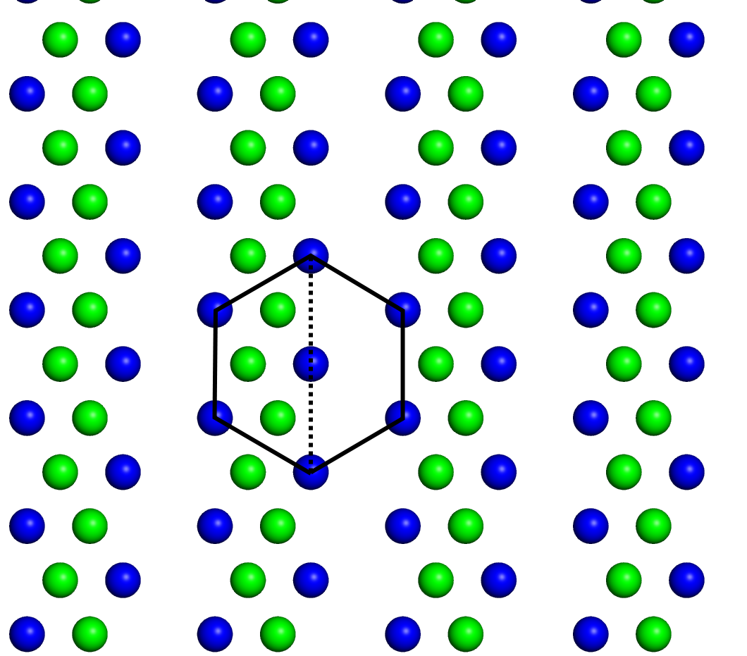
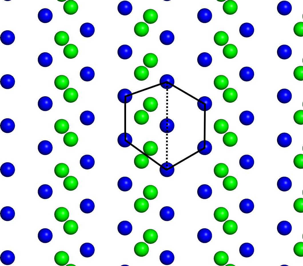
Figure 2: Left panel: structure 1 (identified for $q=0.02$), right panel: structure 2 (identified for $q=0.05$). Blue: charges $Q_{1}$, green: charges $Q_{2}$. Lines highlight the hexagonal units discussed in the text. The dotted lines mark the central axes of the hexagonal units (cf. text).

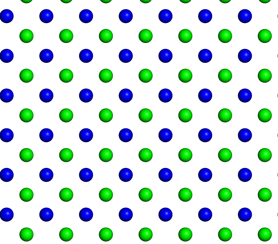
Figure 3: Structure 3 (identified for $q=0.10$). Blue: charges $Q_{1}$, green: charges $Q_{2}$.

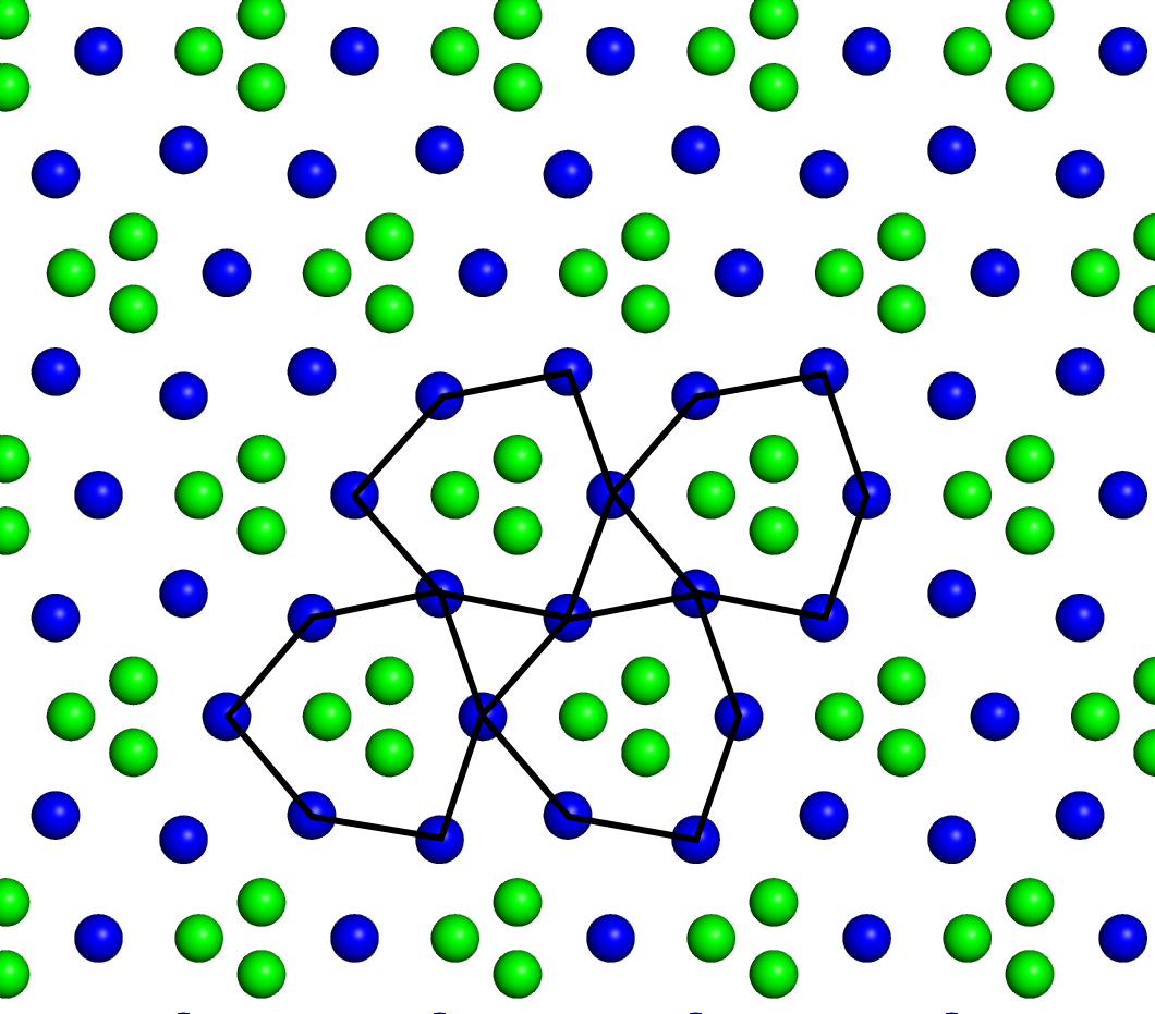
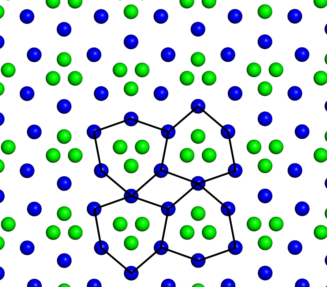
Figure 4: Left panel: structure 4 (identified for $q=0.26$), right panel: structure 5 (identified for $q=0.27$. Blue: charges $Q_{1}$, green: charges $Q_{2}$. Lines highlight the hexagonal units discussed in the text.

The Table provides an overview over the ground state configurations that we have identified for $0\leq q\leq 1$; the structures themselves are depicted in Figures 2 – 5.

Table 1: Overview over the identified ground state configurations and the respective $q$-ranges. The structures themselves are depicted in Figures 2 – 5.

$q$-range	ground state structure
0.00	hexagonal lattice formed by charges $Q_{1}$
$0.00<q\lesssim 0.04$	Structure 1
$0.05\lesssim q\lesssim 0.09$	Structure 2
$0.10\lesssim q\lesssim 0.25$	Structure 3
$0.26\simeq q$	Structure 4
$0.27\lesssim q\lesssim 0.28$	Structure 5
$0.29\lesssim q\lesssim 0.59$	Structure 6
$0.60\lesssim q<1$	phase separation
1.00	hexagonal lattice formed by the
	(indistinguishable) charges $Q_{1}$ and $Q_{2}$

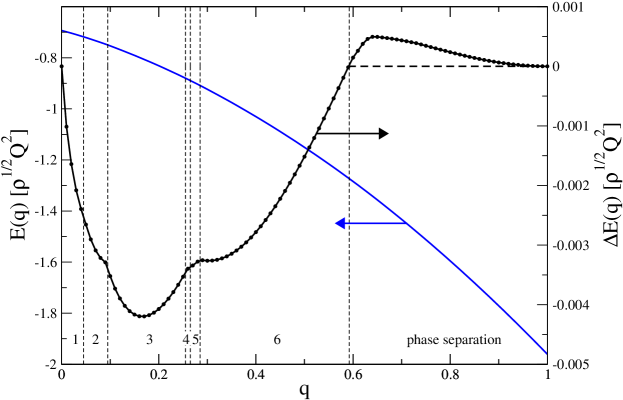
Figure 1: Energy per particle of the ground state configuration, $E(q)$ (blue line), and energy difference (per particle), $\Delta E(q)=[E(q)-E_{0}(q)]$ (black line), with respect to the reference energy, $E_{0}(q)$, as defined in equation (5) as functions of $q$. Vertical broken lines indicate the limits of stability of the six identified non-trivial ground states. The horizontal broken line marks the $q$-values where the phase separated system is the energetically most favourable one.

For $q=0$, charges with non-vanishing nominal values, $Q_{1}$, arrange – as expected – in a hexagonal lattice (not depicted) with number density $\rho_{1}=\rho/2$; the other, chargeless particles do not interact with any particle species and thus occupy arbitrary positions.

For $0<q\lesssim 0.04$, charges $Q_{1}$ form a hexagonal lattice which is to a high degree regular (Structure 1, depicted in the left panel of Figure 2): the order parameter $\Psi_{6}$ varies between $\Psi_{6}(q=0.01)=0.99972$ and $\Psi_{6}(q=0.04)=0.99577$. The deviation from its ideal value, $\Psi_{6}=1$, stems from a slight distortion of these hexagons (highlighted in the corresponding panel): a central ’axis’ (dotted line in the corresponding panel), connecting the ’upper’ and ’lower’ vertices of the hexagon, is formed by two line-segments of equal length; the distances of the vertices left (right) to this central axis from the center of the hexagon differ in their length by less than +4% (-3 %). Thus the left half of the hexagon is slightly larger than its counterpart located to the right of the central axis. This enlarged space is imposed by the fact that this area hosts charges $Q_{2}$, which form a zig-zag pattern within the ground state configuration, oriented parallel to the central axis of the hexagon; within this line, charges $Q_{2}$ are equidistant. The other part of the hexagon, located right to its central axis remains empty.

In the adjacent $q$-range, $0.05\lesssim q\lesssim 0.09$, charges $Q_{1}$ maintain their hexagonal arrangements (Structure 2, displayed in the right panel of Figure 2). As compared to Structure 1, the distortion of the hexagons (highlighted in the corresponding panel) is now considerably more pronounced: $\Psi_{6}(q=0.05)=0.90598$ while $\Psi_{6}(q=0.09)=0.83643$. The ’upper’ and the ’lower’ vertices of the hexagon are still connected via a central axis (dotted line in the corresponding panel), consisting of two line segments of equal length; however, the distances of the vertices left to this central axis from the center of the hexagon are now by up to 21 % longer, while the corresponding distances of the vertices on the opposite side of the axis are less than 5 % shorter. This conceivable asymmetry (see the highlighted hexagon in the corresponding panel) is imposed by the increased nominal value of charge $Q_{2}$: the zig-zag arrangement of particles, observed for this species of charges in Structure 1 has been replaced by a parallel arrangements of pairs of particles which are aligned in the direction of the central axis of the hexagon; while the intra-pair distance is very short, the inter-pair distance is quite large.

In the relatively wide range of $0.10\lesssim q\lesssim 0.25$ the two species of charges arrange in two intertwining, commensurate square lattices (Structure 3, cf. Figure 3). It has to be emphasized that both sublattices remain perfect over the entire $q$-range of stability, i.e., $\Psi_{4}=1$ for $0.10\lesssim q\lesssim 0.25$. The structural stability of this particular ground state is also reflected by the fact that Structure 3 is characterized by the highest energy gain compared to the energy value of the reference structure, $E_{0}(q)$ (see Figure 1).

Around the value $q\simeq 0.26$, charges $Q_{1}$ form hexagonal structural units which are in their shape reminiscent of gems or diamonds. These six-particle rings form in a head-to-tail arrangement parallel lanes: adjacent six-particle rings of neighbouring lanes share vertices, while the remaining edges form equilateral triangles. This ground state is referred to as Structure 4; it is depicted in the left panel of Figure 4 and the six-particle rings are highlighted. Each of the six-particle units hosts in its center an essentially equilateral triangle of charges $Q_{2}$. The positions of the six surrounding charges $Q_{1}$ are imposed by the condition that the smallest distance of these charges from any of the three inner charges ($Q_{2}$) has the same value; this requirement induces the particular shape of the six-particle rings. The triangular arrangements that fill up the interstitial space are not populated by charges $Q_{2}$.

The ground state identified for $0.27\lesssim q\lesssim 0.28$ (denoted as Structure 5 and depicted in the right panel of Figure 4) differs only in one feature from Structure 4: the lanes, formed by the head-to-tail arrangements of the six-particle rings (highlighted in the corresponding panel) are now antiparallel. In this configuration the neighbouring rings of adjacent lanes share edges, which leads now to the formation of rhombic four-particle arrangements which are again void of $Q_{2}$ charges.

Finally, at $q\simeq 0.29$ Structure 6 emerges and remains the ground state over the relatively large interval $0.29\lesssim q\lesssim 0.59$ (see left panel of Figure 5). Its basic unit is an elongated hexagon (highlighted in the corresponding panel): aligned in parallel and sharing edges with neighbouring tiles, they completely cover the two-dimensional space. The direction perpendicular to the longest elongation of this hexagon is considered for the following discussion as the central axis (dotted in the corresponding panel). For Structure 6 this axis is also the symmetry axis of the hexagon. The four edges originating from the central axis have the same lengths, say $l_{1}$; similarly, the remaining two edges of the hexagon (oriented parallel to the central axis) assume another, equal value, say $l_{2}$. Each of these hexagons hosts a pair of charges $Q_{2}$, located on a line perpendicular to the central axis and separated by a distance, which decreases as $q$ is increased. By increasing the charge ratio $q$, $l_{1}$ decreases from $1.297\sqrt{\rho}$ (at $q=0.29$) to $1.269\sqrt{\rho}$ (at $q=0.59$), while $l_{2}$ increases from $1.29\sqrt{\rho}$ (at $q=0.29$) to $1.324\sqrt{\rho}$ (at $q=0.59$). At the cross-over, i.e., $l_{1}\simeq l_{2}$ (observed for $q\simeq 0.36$, our optimization tool identifies a closely related, energetically degenerate structure, denoted as Structure 6’ and depicted in the right panel of Figure 5: now that all edges of the basic hexagon are equal, these units are no longer forced to align in parallel, but are able to chose an alternative, non-parallel arrangement: imposed by the internal angle between edges of the basic hexagon, these units arrange in a grain-like super-structure.

For $0.59\lesssim q<1.00$, we find that $E_{0}(q)<E(q)$ (see Figure 1), indicating that the phase separated particle configuration is energetically more stable than any other ordered structure identified by our optimization tool. Due to the limitation in the number of particles per unit cell, the EA-based search for ground state configurations proposes – depending on the number of particles per cell – configurations with increasing complexity, all of them being characterized by an energy value $E(q)$ that is larger than the corresponding value $E_{0}(q)$. Thus the demixed state, formed by two separate hexagonal, ordered regions and each of them being populated by one species of charge, is the ground state in this $q$-range.

Finally, for $q=1$, we recover the one-component hexagonal monolayer (not displayed).

V Conclusions

In this contribution we have investigated the ground state configurations of an equimolar, binary mixture of classical charged particles (with nominal charges $Q_{1}$ and $Q_{2}$), that self-assemble on a neutralizing plane. Our investigations are based on reliable Ewald summation techniques which allow an efficient evaluation of the ground state energies (= lattice sums). With the help of reliable optimization tools, which are based on ideas of evolutionary algorithms, we are able to identify the ordered ground states of the system: by searching essentially among all possible two-dimensional lattices, this algorithm identifies for a given charge ratio $q=Q_{2}/Q_{1}$ the energetically most favourable particle arrangement. Apart from the expected, trivial hexagonal lattices for $q=0$ and $q=1$, we could identify for $0<q\lesssim 0.59$ in total six ground state configurations.

Quite unexpectedly, these particle arrangements show a remarkable structural complexity which is the result of the energetic competition between the charge-charge interactions. Throughout, a pronounced impact of the weaker charges, $Q_{2}$, on the sublattices formed by the stronger charges, $Q_{1}$, could be observed: this holds even if the corresponding $q$-values are rather small (i.e., $q\simeq 0.05$). Except for a purely square particle arrangement (which is stable over a remarkably large $q$-range and which shows the highest energy gain among all ground states with respect to a suitably defined reference state – see also the discussion about energies below), the ground states can be described on the basis of asymmetric, sometimes strongly distorted six-particle arrangements formed by charges $Q_{1}$, which host in their interior simple two- or three-particle configurations of charges $Q_{2}$. A deeper insight into the mechanisms that govern the formation of ground states is gained by introducing a phase separated reference state, where the two species of charges populate in hexagonal arrangements spatially separated areas. Comparing the energies of our ground state configurations, $E(q)$, with the energy of this reference state, $E_{0}(q)$, we find that these two functions differ by less than $5\times 10^{-3}$, a fact that represents a characteristic fingerprint of the long-range Coulomb interactions. An analysis of this energy difference as a function of $q$ reveals that transitions from one ground state to an adjacent one become visible as (more or less pronounced) kinks in this function. Based on these considerations we could show that for $0.59\lesssim q<1$ the energetically most favourable particle arrangement is the (ideal) phase separated state.

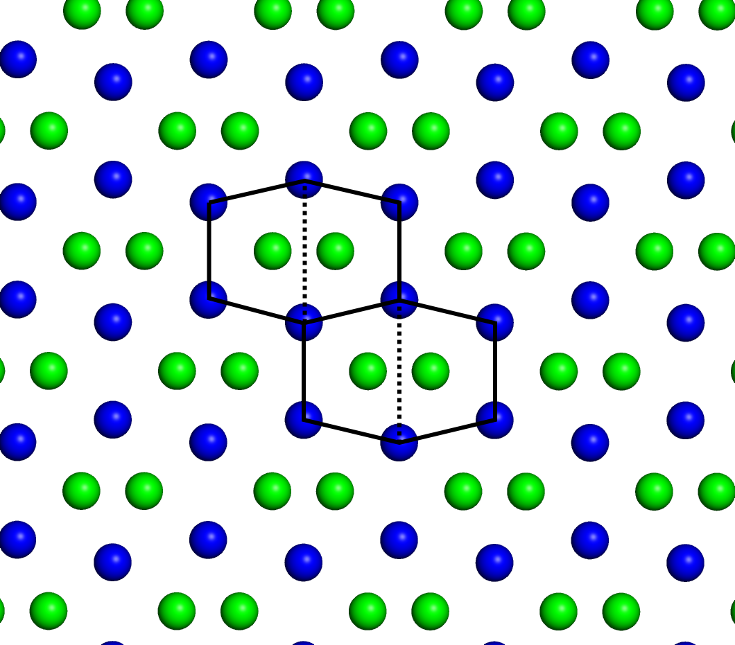
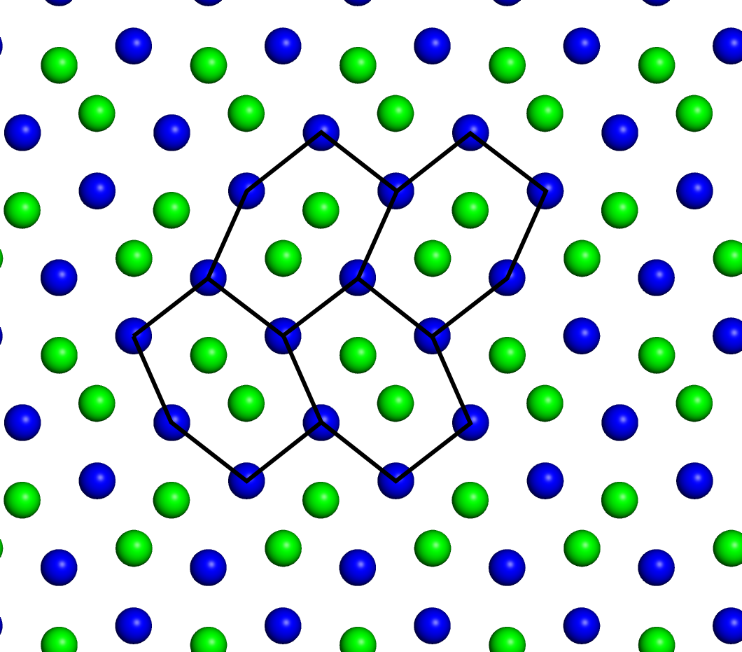
Figure 5: Left panel: structure 6 (identified for $q=0.30$), right panel: structure 6’ (identified for $q=0.35$. Blue: charges $Q_{1}$, green: charges $Q_{2}$. Lines highlight the hexagonal units discussed in the text. The dotted lines mark the central axes of the hexagonal units (cf. text).

References

- (1) Wigner E., Phys. Rev., 1934, 46, 1002.
- (2) Meißner G., Namaizawa H., Voss M., Phys. Rev. B, 1976, 13, 1370.
- (3) Bonsall L., Maradudin A. A., Phys. Rev. B, 1977, 15, 1959.
- (4) Levin Y., Rep. Prog. Phys., 2002, 65, 1577.
- (5) Šamaj L., Trizac E., EPL, 2012, 98, 36004.
- (6) Šamaj L., Trizac E., Phys. Rev. B, 2012, 85, 20513.
- (7) Mazars M., Phys. Rep., 2011, 500, 43.
- (8) Adaptation in Natural and Artificial Systems. Holland J. H., The University of Michigan Press, Ann Arbor, 1975.
- (9) Gottwald D., Kahl G., Likos C., J. Chem. Phys., 2005, 122, 204503.
- (10) Pauschenwein G.J., Kahl G., J. Chem. Phys., 2008, 129, 174107.
- (11) Kahn M., Weis J.J., Likos C.N., Kahl G., Soft Matter, 2009, 5, 2852.
- (12) Kahn M., Weis J.J., Kahl G., J. Chem. Phys., 2010, 133, 224504.
- (13) Fornleitner J., Kahl G., EPL, 2008, 82, 18001.
- (14) Fornleitner J., Lo Verso F., Kahl G., Likos C.N., Soft Matter, 2008, 4, 480.
- (15) Fornleitner J., Lo Verso F., Kahl G., Likos C., Langmuir, 2009, 25, 7836.
- (16) Doppelbauer G., Bianchi E., Kahl G., J. Phys.: Condens. Matter, 2010, 22, 10410.
- (17) Antlanger M., Doppelbauer G., Kahl G., J. Phys.: Condens. Matter, 2011, 23, 404206.
- (18) Doppelbauer G., Noya E.G., Bianchi E., Kahl G., Soft Matter, 2012, 8, 7768.
- (19) Strandburg K.J., Rev. Mod. Phys., 1988, 60, 161.