Sudden and slow quenches into the antiferromagnetic phase of ultracold fermions

Abstract

We propose a method to reach the antiferromagnetic state of two-dimensional Fermi gases trapped in optical lattices: Independent subsystems are prepared in suitable initial states and then connected by a sudden or slow quench of the tunneling between the subsystems. Examples of suitable low-entropy subsystems are double wells or plaquettes, which can be experimentally realized in Mott insulating shells using optical super-lattices. We estimate the effective temperature $T^{*}$ of the system after the quench by calculating the distribution of excitations created using the spin wave approximation in a Heisenberg model. We investigate the effect of an initial staggered magnetic field and find that for an optimal polarization of the initial state the effective temperature can be significantly reduced from $T^{*}\approx 1.7\,T_{c}$ at zero polarization to $T^{*}<0.65\,T_{c}$, where $T_{c}$ is the crossover temperature to the antiferromagnetic state. The temperature can be further reduced by using a finite quench time. We also show that $T^{*}$ decreases logarithmically with the linear size of the subsystem.

I. INTRODUCTION

Ultracold fermions trapped in optical lattices have emerged as ideal model systems to simulate the Hubbard model Zwerger2008 ; Esslinger2010 . Major achievements include the observation of Mott insulating states Joerdens2008 ; Schneider2008 and of short-range antiferromagnetic ordering Esslinger2013 and the simulation thereof Greiner2011 . Currently the observation of long-range antiferromagnetic ordering is the next milestone on the quest to simulate low-temperature phases of the Hubbard model and find answers to open questions such as the origin of high-temperature superconductivity. The main experimental challenge is the reduction of entropy or temperature by at least a factor of two or four, respectively Joerdens2010 .

To achieve this temperature reduction, one can take advantage of the excellent tunability of ultracold atomic systems: Several cooling schemes have been proposed, which should allow to reduce the entropy of the systems (for a review, see Ref. deMarco2011 ). In the scheme proposed here, we make use of the fact that in trapped systems, gapped states can be in thermal contact with gapless states, similarly as in related proposals Capogrosso2008 ; Bernier2009 ; Ho2009 ; Cirac2011 ; Trivedi2011 ; Hulet2012 ; Vekua2011 . As a result, the entropy in the gapped region is strongly reduced and the excitations in the gapless region carry most of the entropy. A prominent example is a band insulating state surrounded by a compressible metallic state.

We propose to transform the central band insulating shell into an antiferromagnetic state by first assembling subsystems featuring precursors of magnetic ordering, followed by a sudden or slow quench connecting the previously independent subsystems. We calculate the effective temperature $T^{*}$ after the quench and compare it with the critical temperature for antiferromagnetic ordering $T_{c}$. The following questions then arise naturally: What is the ideal inital state that minimizes $T^{*}$?

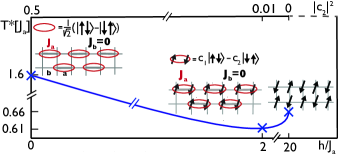
Figure 1: (color online) The effective temperature $T^{*}$ after the sudden quench as a function of the initial state’s coefficient $c_{2}$ or the magnetic field $h$. Arrows represent spins, each red ellipse denotes a singlet state $(|\uparrow\downarrow\rangle-|\downarrow\uparrow\rangle)/\sqrt{2}$ and ellipses surrounding arrows denote optimally polarized singlet states $0.99|\uparrow\downarrow\rangle-0.12|\downarrow\uparrow\rangle$. $J_{a}$ (bold) and $J_{b}$ (thin lines) are the intra- and inter-dimer interactions.

How does $T^{*}$ depend on the size of the initial state and on the speed of the quench?

To answer the first question, we consider a double well as the simplest non-trivial subsystem, see Fig. 1. An array of double wells can be created in a dimerized lattice Phillips2007 ; Bloch2008 ; Esslinger2013 , starting from a band insulating state and separating the sites employing e.g. a frequency doubled optical lattice Bloch2008 . In our limit of strong onsite interaction $U$, the atoms are treated as Heisenberg spins with very weak inter-dimer interactions $J_{b}$ and strong intra-dimer coupling $J_{a}$. Naively, one might think that the ideal choice for the initial state of the subsystem would be a singlet state $|\psi\rangle=c_{1}|\uparrow\downarrow\rangle+c_{2}|\downarrow\uparrow\rangle$ with $|c_{1,2}|^{2}=1/2$, since this is the groundstate. However, this state has zero staggered magnetization and hence only a small overlap to the $T=0$ antiferromagnetic state. At the other extreme, a classical Néel state with $|c_{2}|=0$ already contains a preferred direction of broken symmetry and staggered magnetism. The drawback here is the perfect ordering, which is not present in larger systems even at $T=0$ due to quantum fluctuations. The optimal state is a partially polarized state, with $|c_{2}/c_{1}|\approx 8$, featuring $T^{*}\approx 0.61\,J_{a}$.

In the two-dimensional systems at finite temperature considered here, only short range order with exponentially decaying correlations at finite temperature exists. The correlation length $\xi(T)=A\exp{(2\pi\rho_{s}/k_{B}T)}$ diverges exponentially for $T\rightarrow 0$. Here $\rho_{S}=0.199$ is the renormalized spin-stiffness constant at $T=0$ and $A\approx 0.276$ Ding1990 ; Manousakis1991 ; Chakravarty1989 . However, the regime for which the correlation length $\xi(T)$ is larger than the lattice spacing $d$, is referred to as the antiferromagnetic (AF) regime. The crossover temperature $T_{c}\approx 0.97\,J$ is defined as $\xi(T_{c})=d$. As we show below, the optimal initial state of a product state of subsystems of size $L$ resembles the finite-temperature state in the following way: The optimal state of the subsystems also has to have a nonzero magnetization, in analogy to the short-range order of the second-order phase transition, and the optimal temperature $T^{*}$ approximately fulfills $\xi(T^{*})\approx L$. The initial state therefore consists of “patches” of short-range order of length $L$, in analogy to the short-range ordered AF state with a correlation length $\xi(T)$. This implies that even when increasingly larger magnetically ordered subsystems with corresponding correlation lengths $\xi^{*}$ are prepared, the effective temperature $T^{*}$ obtained after the quench only decreases logarithmically with $\xi^{*}$, as we show numerically. We note that the correlation length $\xi(T)$ is experimentally visible in the broadening of the structure factor peaks that are obtained via Bragg scattering, in addition to technical broadening.

Our scheme has two major advantages over related schemes: Firstly, no significant redistribution of atoms is required Bernier2009 ; Ho2009 . Such a redistribution is expected to cause severe problems due to the extremely slow mass flow in the Mott insulating regime Chin2010 . Secondly, the high entropy shell surrounding the central region of interest does not necessarily have to be removed: In this case, the timescale of the quench and the subsequent thermalization must be shorter than the time for the entropy to leak back into the central region. This condition will limit the correlation length, but at the same time avoid the need for a removal step Bernier2009 , which is technically very challenging and has not yet been demonstrated experimentally. All ingredients necessary for the implementation of this proposal have already been experimentally demonstrated Phillips2007 ; Bloch2008 ; Esslinger2013 . Merging plaquettes to create a state of fermionic pairs has been discussed in Ref. Rey2009 . Our scheme is closely related to the work by Lubasch and coworkers Cirac2011 , where only double well subsystems initialized in singlet states are considered.

Throughout the paper, we consider fermions in the strongly repulsive coupling regime $U\gg t$, where $t$ is the tunneling matrix element. The system is hence well described by the two-dimensional Heisenberg spin Hamiltonian

$$H=J_{a}\sum_{{\langle ij\rangle}_{a}}\textbf{S}_{i}\textbf{S}_{j}+J_{b}\sum_{{\langle ij\rangle}_{b}}\textbf{S}_{i}\textbf{S}_{j}-\sum_{i}h_{i}S_{i}^{z},$$ (1)

where $\langle ij\rangle_{a/b}$ means summation over nearest neighbours along bonds $a$ and $b$, respectively, and $\textbf{S}_{i}$ is the spin-$1/2$ operator. We set $\hbar\equiv 1$ and $k_{B}\equiv 1$. The exchange couplings $J_{a/b}=4t_{a/b}^{2}/U>0$ quantify interactions $J_{a}$ between spins in a subsystem and interactions $J_{b}$ between subsystems. $t_{a/b}$ are the tunneling energies within/between subsystems. $h_{i}=(-1)^{i}h$ denotes the staggered magnetic field pointing along the $z$ axis. We focus on staggered magnetic fields with a spatially constant amplitude $h$ but also touch briefly on the case with a spatially inhomogeneous amplitude in section IV.A. Changing the ratio $g\equiv J_{b}/J_{a}$, the system undergoes a second order phase transition. For columnar and for staggered dimerization it occurs at $g_{c}=0.38$ Sachdev2000 and $g_{c}=0.396$ Jiang2013 , respectively. For $g>g_{c}$ the groundstate has Néel order, and for $T<T_{c}$ the system is in the so-called renormalized classical regime. For $g<g_{c}$ and for $T<\Delta$ the system in the quantum disordered region with a paramagnetic ground state Chakravarty1989 ; Sachdev2000 , where $\Delta$ is the energy gap of the state.

We perform calculations for different initial subsystems such as double wells, $2\times 2$ plaquettes, $Z$-shaped and larger $n\times m$ subsystems, see Fig. 2b. The subsystems are always prepared in the groundstate of (1) with $J_{b}=0$. To estimate the effective temperature, we assume that only low-energy modes are excited during the slow quench. Using linear spin-wave theory AA we analytically (numerically) estimate the temperature $T^{*}$ for small (large) subsystems. We study how the effective temperature $T^{*}$ depends on the quench time $\tau$ and present analytical results for slow changes.

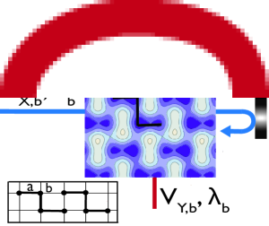
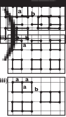
Figure 2: (color online) (a) Contour plot of the Z-shape optical lattice. Beams $\bar{X}$, $X$ propagate along the same axis and beam $Y$ along an axis perpendicular to that axis. Beam $Y$ interferes with beam $X$. Lighter regions correspond to higher potential energy and darker to lower energy. We choose $V_{\bar{X},b}=V_{Y,b}=1,V_{X,b}=0.2$, $V_{X,r}=V_{Y,r}=0.3$ and $\phi_{1}=\pi/2,\,\,\phi_{2}=\pi/4.$ (b) Schematic pictures of dimers (i), $2\times 2$ plaquettes (ii) and $3\times 2$ plaquettes (iii).

II. LATTICE GEOMETRY

In our studies we consider several optical lattices, simple square and dimerized lattices as well as plaquette- and $Z$-shaped lattices. Dimerized and plaquette-shaped lattices have already been realised experimentally using super-lattices Bloch2008 ; Bloch2012 or a mixture of interfering and non-interfering lattices Phillips2007 ; Esslinger2013 .

Here we describe a technique to create an array of four-site states in $Z$-shape configuration, see Fig. 2a. This is the most complicated geometry which we still deem realizable with current experimental techniques. Due to the $Z$-shape, a staggered magnetic field can be created employing only a magnetic field gradient pointing along the diagonal axis. The larger $n\times m$ plaquettes depicted in Fig. 2b-iii serve as theoretical constructs to discuss scaling issues.

For each lattice, the fundamental building block is a repulsive cubic optical lattice $V_{\bar{X},Y}(x,y)$ generated by two blue-detuned retro-reflected beams $\bar{X}$ and $Y$, as depicted in Fig. 2a. The two beams have a wavelength of e.g. $\lambda_{b}=532$ nm and a slight frequency offset to avoid mutual interference. In order to make effective bonds along the $x$-direction, an additional retro-reflected beam $X$ along the $x$-direction is used, which interferes with beam $Y$. The resulting potential is $V_{X,Y}(x,y)$. The bonds along the $y$-direction are created by an attractive cubic optical lattice $V_{\lambda_{r}}(x,y)$ formed by two red-detuned retro-reflected beams at a wavelength $\lambda_{r}=2\lambda_{b}$ (beams not shown in Fig. 2a). The resulting trapping potential is presented in the Fig. 2a and given by the equation

$$V(x,y) = V_{\bar{X},Y}(x,y)+V_{X,Y}(x,y)+V_{\lambda_{r}}(x,y)$$

$$= +V_{\bar{X},b}\cdot\cos^{2}(k_{b}x)+V_{Y,b}\cdot\cos^{2}(k_{b}y)$$

$$+V_{X,b}\cdot\cos^{2}(k_{b}x+\phi_{1})$$

$$+2\sqrt{V_{X,b}V_{Y,b}}\cdot\cos(k_{b}x+\phi_{1})\cos(k_{b}y)$$

$$-V_{X,r}\cdot\cos^{2}(k_{r}x)-V_{Y,r}\cdot\cos^{2}(k_{r}y+\phi_{2}),$$

where $V_{\bar{X},b},V_{X,b},V_{Y,b}$ and $V_{X,r},V_{Y,r}$ are the respective lattice depths. They are given in units of the recoil energy $E_{b}=h^{2}/2m\lambda_{b}^{2}$ for $V_{\bar{X},b},V_{X,b},V_{Y,b}$ and $E_{r}=h^{2}/2m\lambda_{b}^{2}$ for $V_{X,r},V_{Y,r}$. $m$ denotes the mass of a single atom.

III. SPIN WAVE THEORY

To describe the final state after the quench and estimate $T^{*}$, we use linear spin-wave theory following Holstein and Primakoff (HP) Holstein1940 , in the notation of Ref. AA . We choose the classical Néel state along the $z$ and $-z$ direction and define the rotated spin $\tilde{\bf S}_{i}\equiv(S_{i}^{x},-S_{i}^{y},-S_{i}^{z})$, for sites $i$ on one sublattice. Then the Hamiltonian reads

$$H=-|J|\sum_{\langle ij\rangle}S_{i}^{z}\tilde{S}_{j}^{z}+\frac{|J|}{2}\sum_{\langle ij\rangle}(S_{i}^{+}\tilde{S}_{j}^{+}+S_{j}^{-}\tilde{S}_{i}^{-}).$$ (3)

where we note that after the quench the spin couplings are equal, i.e., $J_{a}=J_{b}\equiv J$. We now approximate the spins by bosonic operators

$$S_{i}^{+}=\sqrt{2S-n_{i}}a_{i},\,S_{i}^{-}=a_{i}^{\dagger}\sqrt{2S-n_{i}},\,S_{i}^{z}=S-n_{i},$$ (4)

and similarly for $\tilde{\bf S}_{i}$. The operators $a_{i}$, $a_{i}^{\dagger}$ satisfy commutation relations $\left[a_{i},a_{j}^{\dagger}\right]=\delta_{ij}$, and $n_{i}\equiv a_{i}^{\dagger}a_{i}$ is the number of bosons on site $i$. It is limited by $2S$, with $S=1/2$. We expand the square root in Eqs. (4) as $\sqrt{1-n_{i}/2S}\approx 1-\frac{n_{i}}{4S}-\cdots$ and carry out the calculations to the lowest order, i.e., perform the linear spin wave approximation. This leads to an ensemble of non-interacting bosonic modes.

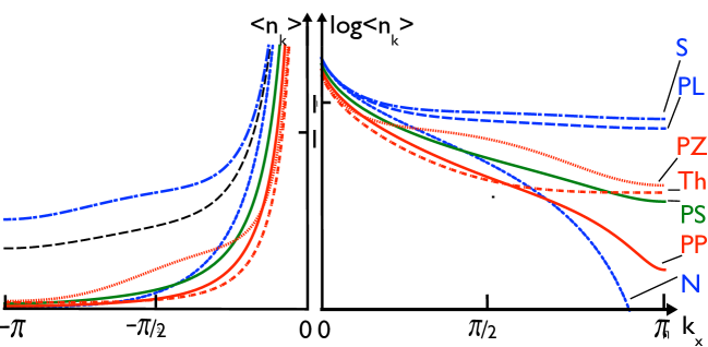
Figure 3: (color online) The average number of excitations $\langle n_{\textbf{k}}\rangle$ on a linear and logarithmic scale as a function of $k_{x}$, for $k_{y}=0$. The initial states are: Néel (N), singlet (S), polarized singlet (PS), plaquette (PL), polarized plaquette (PP), polarized $Z$-state (PZ) and a thermal distribution (Th) with $T=0.554\,J$. For the polarized cases the optimal magnetic field yielding the lowest effective temperature was chosen.

We first insert the linearized bosonic operators of Eq. (4) into the Hamiltonian (3) and use the Fourier transform $a_{\textbf{k}}=\frac{1}{\sqrt{N}}\sum_{i}e^{-i\textbf{k}\textbf{r}_{i}}a_{i}$ where k runs over the first Brillouin zone, $\textbf{k}\in[-\pi/a,\pi/a)^{2}$, where $a$ is the lattice constant, set to $a\equiv 1$. $N$ is the number of lattice sites. The Hamiltonian becomes

$$H=-\frac{NzJS^{2}}{2}+zJS\sum_{\textbf{k}}(a_{\textbf{k}}^{\dagger}a_{\textbf{k}}+\frac{\gamma_{\textbf{k}}}{2}(a_{\textbf{k}}a_{-\textbf{k}}+a_{\textbf{k}}^{\dagger}a_{-\textbf{k}}^{\dagger})),$$

where $\gamma_{\textbf{k}}\equiv\frac{1}{2}(\cos k_{x}+\cos k_{y})$, and $\textbf{k}=(k_{x},k_{y})$. $z$ is the number of the nearest neighbours, $z=2d$, and $d=2$ is the lattice dimensionality. Then we perform a Bogoliubov transformation $a_{\textbf{k}}=u_{\textbf{k}}\alpha_{\textbf{k}}-v_{\textbf{k}}\alpha_{-\textbf{k}}^{\dagger}$, with $u_{k}=\cosh\theta_{k}$ and $v_{k}=\sinh\theta_{k}$, where the $\alpha_{\textbf{k}}$ are bosonic operators. To cancel anomalous terms in the Hamiltonian we choose $\tanh 2\theta_{\textbf{k}}=-\gamma_{\textbf{k}}$. The Hamiltonian now has the desired diagonal form

$$H_{LSW}=-\frac{NzJS^{2}}{2}+\sum_{\textbf{k}}\omega_{\textbf{k}}(\alpha_{\textbf{k}}^{\dagger}\alpha_{\textbf{k}}+\frac{1}{2}),$$ (5)

where $\omega_{\textbf{k}}=JSz\sqrt{1-\gamma_{\textbf{k}}^{2}}$ is the spin-wave dispersion relation. Near $\textbf{k}=\{0,0\}$ and $\textbf{k}=\{\pi,\pi\}$ the dispersion is linear with $\omega_{\textbf{k}}\approx JSz\mid\textbf{k}\mid$ and $\omega_{\textbf{k}}\approx JSz\mid\textbf{k}-(\pi,\pi)\mid$, respectively. These two Goldstone modes reflect the broken symmetry of the antiferromagnetic state. Due to the absence of a gap the creation of excitations cannot be avoided even for a slow quench. The staggered magnetization $M=\frac{1}{N}\sum_{i}(-1)^{i}\langle S_{i}^{z}\rangle$ for spin-$1/2$ in the linear spin-wave approximation is $M\approx 0.303$ Manousakis1991 ; AA , so quantum fluctuations lead to a reduction to about 60$\%$ of the classical value. Numerical and theoretical studies of the staggered magnetization in the infinite-lattice extrapolation for spin-$1/2$ Heisenberg models have found that $M\sim 0.25-0.4$ Manousakis1991 .

IV. SUDDEN QUENCH

We now describe the method to determine the effective temperature $T^{*}$ after the quench. In short, we calculate the momentum distribution of spin waves created in the quench using linear spin-wave theory, $\langle n_{\textbf{k}}\rangle=\sum_{i,j}c_{i}^{*}c_{j}\langle i|\alpha_{\textbf{k}}^{\dagger}\alpha_{\textbf{k}}|j\rangle$, where the summation is over the basis states $|i\rangle$ of the subsystem, and $|\Psi\rangle\equiv\sum_{i}c_{i}|i\rangle$ is the groundstate. The average number of excitations $\langle n_{\textbf{k}}\rangle$ as a function of $k_{x}$ (and $k_{y}=0$) for various geometries is plotted in Fig. 3. The energy of the system, compared to the groundstate, after the quench is given by $\langle E\text{$\rangle$=}\sum_{\mathbf{k}}\langle n_{\textbf{k}}\rangle\omega_{k}$. Since the system is isolated, the energy after the quench is conserved. The effective temperature $T^{*}$ is then defined to be the temperature of a thermal distribution having the same energy $\langle E^{th}\text{$\left(T^{*}\right)\rangle$=}\sum_{\mathbf{k}}\langle n_{\textbf{k}}^{th}(T^{*})\rangle\omega_{k}$. An alternative measure for the temperature scale $T_{k}^{*}$ can be defined by finding the thermal distribution $\langle n_{\textbf{k}}^{th}(T_{k}^{*})\rangle$ which matches the post-quench distribution $\langle n_{\textbf{k}}\rangle$ at small momenta, yielding $T_{k}^{*}=\lim_{k\rightarrow 0}\langle n_{\textbf{k}}\rangle\omega_{k}$. We note that this limit is well-defined, because for the cases we discuss here, the limit is independent of how ${\bf k}$ approaches zero. We use the former definition $T^{*}$, since it takes into account not only low energy but rather all excitations created. We note that $T_{k}^{*}$ appears when we consider slow quenches in section VI.

Table 1: TAB. I. The minimal energy $\langle E\rangle$ and the minimal temperatures $T^{*}$ and $T_{k}^{*}$ at optimal polarization. For effective temperatures $T^{*}<T_{c}=0.97\,J$ Chakravarty1989 ; Manousakis1991 ; Ding1990 antiferromagnetic ordering is expected.

A. Homogeneous magnetic field

The precise protocol of the quench is as follows: Initially, we assume that the coupling between subsystems is $J_{b}=0$, and the amplitude of the staggered magnetic field $h$ can chosen freely. The quench is initiated by suddenly increasing the coupling between subsystems, i.e., setting $J_{b}=J_{a}$. At the same time the magnetic field is turned off. The groundstate before the quench $|\Psi\rangle$ is found by solving the Heisenberg Hamiltonian in eq. (1) in linear spin wave approximation, see eq. (5). The momentum distribution is determined by evaluating $\langle\Psi|\alpha_{\textbf{k}}^{\dagger}\alpha_{\textbf{k}}|\Psi\rangle$. We perform analytical calculations for the Néel state, singlet state, $2\times 2$ plaquette and $Z$-shape state. Details of the calculations are presented in the Appendix. For the larger $n\text{$\times$}m$ plaquettes we carry out numerical calculations using exact diagonalization. Table I summarizes the effective temperatures found for the different configurations. We observe that with the proposed scheme the regime of antiferromagnetic correlations can be easily reached, with e.g. $T^{*}\approx 0.63\,T_{c}$ for optimally polarized singlets. There is good agreement between the two effective temperatures for optimally polarized states, which minimize high-energy excitations. The much larger discrepancy for unpolarized states stems from the fact that only the low energy part of the distribution is used to determine $T_{k}^{*}$.

Fig. 4 depicts numerical results for systems up to 20 spins in a $5\times 4$ configuration. As the magnetic field increases, the effective temperature of the system decreases up to the minimum value $T^{*}$. After exceeding the optimal value of the magnetic field all curves tend towards the temperature of the classical Néel state $T^{*}\approx 0.66\,J$. The plot shows that the magnetization and the effective temperature go to zero with increasing size of the subsystem. We find that $T^{*}$ depends weakly on the subsystem size, possibly indicating logarithmic scaling.

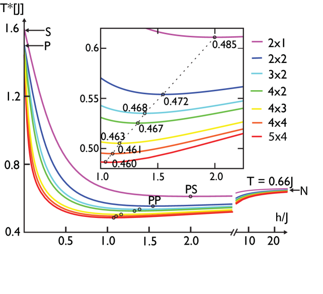
Figure 4: (color online) The effective temperature $T^{*}$ as a function of the magnetic field for larger plaquette subsystems consisting of $m\times n$ sites. The inset shows the regime of $h/J_{a}\in[1.0-2.5]$. The circles mark the minimal effective temperature for each lattice geometry and the labels indicate the corresponding staggered magnetization $M=\frac{1}{N}\sum_{i}\langle S_{i}^{z}\rangle$. It should approach the groundstate value $M\approx 0.303$ of the linear spin-wave approximation as the system size goes to infinity. The dotted line is a guide to the eye. The configuration labels conform to the nomenclature in Fig. 3.

The explanation of this behaviour lies in the dependence of the correlation length on the temperature $\xi(T^{*})$. Inverting this formula and assuming that the correlation length is comparable to the linear size of a subsystem yields $T^{*}=\frac{2\pi\rho_{S}}{\log{(L/A)}}$, where we choose $L=\sqrt{m\cdot n}$ as the length scale of the subsystem. The curve is plotted in Fig. 5a and compared to our numerical results (dots). We note that a $2\times 2$ plaquette and the $Z$-system give almost the same energy $T^{*}$. This is consistent with the hypothesis that $T^{*}$ scales only with the linear system size $L$.

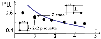
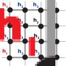
Figure 5: (color online) (a) The minimal temperature $T^{*}$ as a function of the linear size of subsystems $L$. There is reasonable agreement between the numerical results (dots) with the expected logarithmic scaling (continuous line) expected from theory with $\rho_{S}=0.199$ and $A=0.276$ Ding1990 . (b) Distribution of inhomogenous staggered magnetic fields over a $4\times 4$ plaquette, the field values $h_{1},h_{2},h_{3}$ characterize the distribution.

B. Inhomogeneous magnetic field

So far we only treated the polarization of the initial state by a staggered magnetic field of constant amplitude $h$. Now we take into account a site-dependent staggered magnetic field. We consider only the case of a $4\times 4$ plaquette. The magnetic field on each plaquette is distributed in the way shown in Fig. 5b, with alternating polarity on adjacent sites. The total energy $\langle E\rangle$ is minimized by varying the three parameters $h_{1},h_{2},h_{3}$. We find that the lowest energy corresponds to the case where the outer sites of the plaquette are subjected to a higher magnetic field than those in the center. The energy reaches its minimum value $T_{inh}^{*}$ for $h_{1}/J=1,h_{2}/J=0.7,h_{3}/J=0.45$. However, the reduction in effective temperature with respect to the $4\times 4$ plaquette in a homogeneous staggered field by only $0.003\,J$ to $T_{inh}^{*}=0.492\,J$ is rather small.

VI. SLOW QUENCH

In this section we discuss the effect of a finite quench time $\tau$ on the effective temperature. We consider Néel, singlet, optimally polarized singlet states and optimally polarized $2\times 2$ plaquettes in a homogeneous staggered magnetic field. The system is prepared in the same way as in the sudden quench, but the interaction $J_{b}$ between subsystems is turned on within a time interval $\tau$, and the magnetic field $h$ is turned off smoothly on the same time scale. To estimate the effective temperature we make the simplifying assumption that modes with frequency $\omega_{\textbf{k}}>1/\tau$ adapt adiabatically to the parameter changes whereas modes with $\omega_{\textbf{k}}<1/\tau$ are populated as in a sudden quench. The total energy after the quench can then be calculated as $\langle E(\tau)\rangle=\sum_{\textbf{k}}\omega_{k}\langle n_{k}\rangle\Theta(\omega_{\textbf{k}}-1/\tau)$. As before, we find $T^{*}$ by finding the thermal distribution having an energy $\langle E(\tau)\rangle$. As shown in Fig. 6, the effective temperature drops rapidly with increasing quench time. Moreover, the effective temperatures for Néel and singlet case approach each other since their excitation densities at small momenta approach the same value.

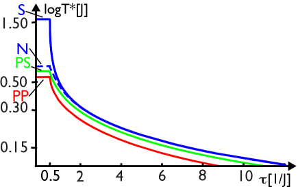
Figure 6: (color online) The effective temperature $T^{*}$ as a function of the quench time $\tau$ on a log-lin scale. The different configurations are labeled as in previous figures. As $\tau$ increases, the effective temperature $T^{*}$ quickly approaches power-law scaling, $T^{*}\sim(T_{k}^{*}/\tau^{2})^{1/3}$.

It is instructive to find the scaling of the effective temperature with quench time in the limit of slow quenches. As it turns out, the effective temperature $T^{*}$ is related to the temperature scale $T_{k}^{*}$ associated with the low-frequency excitations and the sweep time according to $T^{*}\propto\left(\frac{T_{k}^{*}}{\tau^{2}}\right)^{1/3}$. To show this, we consider the limit in which only modes with $\textbf{k}\approx 0$ are occupied, which have a linear dispersion $\omega_{\textbf{k}}\sim|\textbf{k}|$ and consequently an excitation probability $\langle n_{\textbf{k}}\rangle\approx T_{k}^{*}/\omega_{\textbf{k}}$. This gives the following dependence of the total energy on $\tau$:

$$\langle E^{ad}(\tau)\rangle=\frac{1}{(2\pi)^{2}}\int\limits_{\omega_{\textbf{k}<1/\tau}}d^{2}\textbf{k}\,\omega_{k}\langle n_{\textbf{k}}\rangle=\frac{1}{4\pi}\frac{T_{k}^{*}}{\tau^{2}}.$$ (6)

We can compare this energy to the thermal energy for small temperatures:

$$\langle E_{T\rightarrow 0}^{th}\rangle=\frac{1}{(2\pi)^{2}}\int\limits_{0}^{\textbf{k}_{cut}}d^{2}\textbf{k}\,\omega_{k}\langle n_{\textbf{k}}^{th}\rangle=\zeta(3)\frac{T^{*^{3}}}{\pi},$$ (7)

where we again use that for $k\rightarrow 0$ the spin wave spectrum is linear and $\zeta(3)\approx 1.2$ is the Riemann zeta function. Equating these energies we find that for slow quenches the effective temperature changes according to $T^{*}=\left(\frac{1}{4\zeta(3)}\frac{T_{k}^{*}}{\tau^{2}}\right)^{1/3}$. In this limit, the figure of merit to be optimized is thus $T^{*}_{k}$. We note that for even slower quenches, this power law behavior will eventually be controlled by the critical point at $g_{c}$. In this limit, the power-law exponent would be replaced by critical exponents.

VII. SUMMARY

In conclusion, we have proposed a method and a specific experimental realization to reach the antiferromagnetically ordered state by preparing very low entropy subsystems, which do not interact initially. The subsystems are merged by either sudden or slow quenches of the interaction, where slower quenches result in significantly lower effective temperatures. The effective temperature is calculated within linear spin-wave theory and we observe that it reduces with increasing linear subsystems size. Assuming that the subsystem size determines the correlation length of the resulting antiferromagnetic state, we expect logarithmic scaling. Additionally, we find that the effective temperature can be reduced if the subsystems are prepared with optimal polarization, closely resembling the target state. We expect that these insights will be very useful to attain antiferromagnetic ordering in experiments employing double well or plaquettes type geometries. As shown in Sect. II, the method can be implemented with current technology. Furthermore, the principle that is outlined here, i.e., to assemble subsystems with precursors of the desired short-range order, can also be applied to the construction of other many-body states in ultracold atom systems.

We acknowledge support from the Deutsche Forschungsgemeinschaft through the SFB 925 and the Landesexzellenzinitiative Hamburg, which is supported by the Joachim Herz Stiftung.

APPENDIX

In our analytical computations we consider the following states:

1. Classical Néel state. This state is a product state of spins up $|\uparrow\rangle$ and spins down $|\downarrow\rangle$ ordered in a checkerboard $|0\rangle\equiv|\uparrow\downarrow\uparrow\downarrow...\rangle$.

2. Polarized singlet state. This is a product state of singlets which are arranged as shown in picture Fig.2b i. We represent it by the formula:
   $\Big{(}\prod_{\text{i}}(c_{1}-c_{2}\alpha_{i,1}^{\dagger}\alpha_{i,2}^{\dagger})\Big{)}|0\rangle$.
   In the presence of nonzero $h$, the coefficients $c_{1},c_{2}$ are generally not equal to each other only for $h=0$, $c_{1}=c_{2}$, and the standard singlet state is recovered by putting $c_{1}=1/\sqrt{2}$.
   

3. Polarized 2$\times$2 plaquette state. This is a product state of $2\times 2$ plaquettes which are arranged as shown in picture Fig.2b ii. We represent it by the formula:
   $\Big{(}\prod_{i}(c_{1}+c_{2}\prod_{j=1}^{4}\alpha_{i,j}^{\dagger}+c_{3}\sum_{j=1}^{4}\alpha_{i,j}^{\dagger}\alpha_{i,j+1}^{\dagger})\Big{)}|0\rangle$. For $h=0$ the coefficients are following $c_{1}=c_{2}=-\frac{1}{\sqrt{3}},c_{3}=\frac{1}{2\sqrt{3}}$.
   

4. Polarized $Z$-state. This is a product state of $Z$-states which are arranged as shown in picture Fig.2a. We represent it by the formula:
   $\Big{(}\prod_{i}(c_{1}+c_{2}\prod_{j=1}^{4}\alpha_{i,j}^{\dagger}+c_{3}\alpha_{i,2}^{\dagger}\alpha_{i,3}^{\dagger}+c_{4}\alpha_{i,1}^{\dagger}\alpha_{i,4}^{\dagger}+c_{5}(\alpha_{i,1}^{\dagger}\alpha_{i,2}^{\dagger}+\alpha_{i,3}^{\dagger}\alpha_{i,4}^{\dagger}))\Big{)}|0\rangle$

In all above states $|0\rangle$ is the classical Néel state , $\alpha_{i}$, $\alpha_{i}^{\dagger}$ are the annihilation and creation bosonic quasiparticle operators at the lattice site $i$. They are Fourier transformed operators discussed before in the part ’Spin wave theory.’ All states are normalised, $\sum_{i}|c_{i}|^{2}=1$.
The momentum distributions of Bogoliubov excitations created in the sudden quench for the above states are following:

1. For Néel state,

   $$\langle n_{\textbf{k}}\rangle=\frac{1}{2\sqrt{1-\gamma_{\textbf{k}}^{2}}}-\frac{1}{2},$$ (8)

2. For polarized singlet state

   $$\left\langle n_{\textbf{k}}\right\rangle=\frac{c_{2}^{2}+\frac{1}{2}-\gamma_{\textbf{k}}c_{2}\sqrt{1-c_{2}^{2}}\cos{k_{x}}}{\sqrt{1-\gamma_{\textbf{k}}^{2}}}-\frac{1}{2}$$ (9)

3. For polarized 2$\times$2 plaquette state

   $$\left\langle n_{\textbf{k}}\right\rangle=\frac{f_{1}(\textbf{c})}{2\sqrt{1-\gamma_{\textbf{k}}^{2}}}-\frac{1}{2}+2c_{3}^{2}\sin{k_{x}}\sin{k_{y}},$$ (10)

   where $\textbf{c}=(c_{1},c_{2},c_{3})$ and

   $$f_{1}(\textbf{c}) = 2c_{2}^{2}+4c_{3}^{2}(1+\cos k_{x}\cos k_{y})+$$

   $$(\cos k_{x}+\cos k_{y})^{2}(c_{2}c_{3}+c_{1}c_{3})+1,$$

4. For polarized $Z$-state,
   

   $$\left\langle n_{\textbf{k}}\right\rangle=\frac{f_{2}(\textbf{c})}{2\sqrt{1-\gamma_{\textbf{k}}^{2}}}-\frac{1}{2},$$ (12)

   where $\textbf{c}=(c_{1},...,c_{5})$ and $f_{2}(\textbf{c})=\sum_{i=1}^{5}C_{i}(\textbf{c})$
   

   $$C_{1}(\textbf{c}) = 1+2(c_{2}^{2}+c_{5}^{2})+c_{3}^{2}+c_{4}^{2}$$

   $$C_{2}(\textbf{c}) = 2(c_{3}+c_{4})B_{5}\cos{(k_{x}-k_{y})}$$

   $$C_{3}(\textbf{c}) = 2\gamma_{\textbf{k}}(c_{1}+c_{2})c_{5}\cos k_{x}$$ (13)

   $$C_{4}(\textbf{c}) = \gamma_{\textbf{k}}(c_{2}c_{3}+c_{1}c_{5})\cos{(2k_{x}-k_{y})}$$

   $$C_{5}(\textbf{c}) = \gamma_{\textbf{k}}(c_{1}c_{3}+c_{2}c_{5})\cos k_{y}.$$

In all above formulas $\gamma_{\textbf{k}}=\frac{1}{2}(\cos{k_{x}}+\cos{k_{y}})$.

Now we calculate the total energy after the sudden quench, $\langle E\rangle=\sum_{\textbf{k}}\omega_{\textbf{k}}\langle n_{\textbf{k}}\rangle$ in all above states, $\omega_{\textbf{k}}$ is the spin wave dispersion. Energies in the thermodynamic limit are the following:

1. For Néel state, $\langle E\rangle\approx 0.158$.

2. For polarized singlet state,

   $$\langle E\rangle\approx 2c_{2}^{2}+\frac{1}{2}c_{2}\sqrt{1-c_{2}^{2}}+0.16.$$ (14)

3. For polarized 2$\times$2 plaquette state,

   $$\langle E\rangle\approx 2(c_{2}^{2}+2c_{3}^{2})+(c_{2}c_{3}+c_{1}c_{3})+0.16.$$ (15)

4. For polarized $Z$-state

   $$\langle E\rangle\approx 2(c_{2}^{2}+c_{5}^{2})+c_{3}^{2}+c_{4}^{2}+$$ (16)

   $$\frac{1}{4}(c_{1}c_{3}+c_{2}c_{4}+2c_{1}+2c_{2})+0.16.$$

Above energies are convex functions of $c_{i}$’s so they can be optimized over the external magnetic field $h$. The Lagrangian multipliers are used to estimate their minima. Energies with optimal magnetic field $h$ are compared to the energy of thermal distribution with temperature $T^{*}$ in the thermodynamic limit, $\langle E^{th}\rangle=\frac{1}{4\pi^{2}}\int d^{2}\textbf{k}\,\omega_{\textbf{k}}\langle n_{\textbf{k}}^{th}(T^{*})\rangle$. The resulting temperature is denoted as $T^{*}$.
Now we approximate the effective temperature $T^{*}$ for an adiabatic quench. In this case we calculate the number of spin waves in the long-wavelength limit $\langle n_{{k_{x}}}\rangle\equiv\langle n_{\textbf{k}}\rangle_{k_{x}\rightarrow 0}$ (we set $k_{y}=0$):

1. For Néel state, $\langle n_{k_{x}}\rangle=\frac{1}{2\sqrt{1-\gamma_{\textbf{k}}^{2}}}$.

2. For polarized singlet state, $\langle n_{k_{x}}\rangle=\frac{g_{1}(c_{2})}{\sqrt{1-\gamma_{\textbf{k}}^{2}}},$ where $g_{1}(c_{2})=c_{2}^{2}+\frac{1}{2}-c_{2}\sqrt{1-c_{2}^{2}}$.

3. For polarized 2$\times$2 plaquette state, $\left\langle n_{k_{x}}\right\rangle=\frac{g_{2}(\textbf{c})}{\sqrt{1-\gamma_{k}^{2}}},$ where $\textbf{c}=(c_{1},c_{2},c_{3})$ and

   $$g_{2}(\textbf{c})=(c_{2}^{2}+2c_{3}^{2})+2c_{3}^{2}+2(c_{2}c_{3}+c_{1}c_{3})+\frac{1}{2}.$$ (17)

4. For polarized $Z$-state, $\left\langle n_{k_{x}}\right\rangle=\frac{g_{3}(\textbf{c})}{\sqrt{1-\gamma_{k}^{2}}}$,
   where $\textbf{c}=(c_{1},...,c_{5})$ and

   $$g_{3}(\textbf{c})=\frac{1}{2}(2c_{2}^{2}+\sum_{i=3}^{5}c_{i}^{2})+\frac{1}{2}((c_{1}+c_{2})(c_{3}+c_{4}))+c_{5}\sum_{i=1}^{4}c_{i}+\frac{1}{2}.$$ (18)

Since $g_{i}(\textbf{c})$ are convex functions, there is a magnetic field which optimizes $\langle n_{k_{x}}\rangle$. We use again the Lagrangian multipliers to find minima of $\langle n_{k_{x}}\rangle$. We notice that $\langle n_{k_{x}}\rangle$ diverges the same way as a thermal distribution for small energies $\langle n_{\textbf{k}}^{th}\rangle\approx\frac{T^{*}}{\omega_{k}}$. Comparing them we obtain the minimal temperature $T_{k_{x}}^{*}$.

References

- (1) I. Bloch, J. Dalibard, W. Zwerger, Rev. Mod. Phys. 80, 885 (2008).
- (2) T. Esslinger, Annu. Rev. Condens. Matter Phys. 1, 129 (2010).
- (3) R. Jördens et al., Nature 455, 204 (2008).
- (4) U. Schneider et al., Science 322, 1520 (2008).
- (5) R. Jördens et al., Phys. Rev. Lett. 104, 180401 (2010).
- (6) D. Greif, T. Uehlinger, G. Jotzu, L. Tarruell, T. Esslinger, Science 340, 1307 (2013).
- (7) J. Simon, W. S. Bakr, R. Ma, M. E. Tai, P. M. Preiss, M. Greiner, Nature 472, 307 (2011).
- (8) D. C. McKay, B. deMarco, Rep. Prog. Phys. 74, 054401 (2011).
- (9) B. Capogrosso-Sansone, S. G. Söyler, N. Prokof’ev, B. Svistunov, Phys. Rev.A 77, 015602 (2008).
- (10) J.-S. Bernier et al, Phys. Rev.A 79, 061601 (2009).
- (11) T.-L. Ho, Q. Zhou, Proc. Natl. Acad. Sci. U.S.A. 106, 6916 (2009).
- (12) M. Lubasch, V. Murg, U. Schneider, J. I. Cirac, and M.-C. Bañuls, Phys. Rev. Lett. 107, 165301 (2011).
- (13) T. Paiva, Y. L. Loh, M. Randeria, R. T. Scalettar, N. Trivedi, Phys. Rev. Lett. 107, 086401 (2011).
- (14) C. J. M. Mathy, D. A. Huse, R. G. Hulet, Phys. Rev. A 86, 023606(R) (2012).
- (15) M. Colomé-Tatché, C. Klempt, L. Santos, T. Vekua, New J. Phys. 13, 113021 (2011).
- (16) M. Anderlini et al., Nature 448, 452 (2007).
- (17) S. Trotzky et al., Science 319, 295 (2008).
- (18) S. Chakravarty, B. I. Halperin, D. R. Nelson, Phys. Rev. B 39, 2344 (1989); A. V. Chubukov, S. Sachdev, J. Ye, Phys. Rev. B 49, 11919 (1994).
- (19) E. Manousakis, Rev. Mod. Phys. 63, 1 (1991).
- (20) H. Q. Ding and M. S. Makivić, Phys. Rev. Lett. 64, 1449 (1990).
- (21) C.-L. Hung, X. Zhang, N. Gemelke, C. Chin, Phys. Rev. Lett. 104, 160403 (2010).
- (22) S. Sachdev, Science 288, 475 (2000).
- (23) F.-J. Jiang, arXiv:1307.6104 (2013).
- (24) A. Auerbach, Interacting Electrons and Quantum Magnetism, (Springer-Verlag, New York, 1998).
- (25) S. Nascimbène et al., Phys. Rev. Lett. 108, 205301 (2012).
- (26) T. Holstein, H. Primakoff, Phys. Rev. 58, 1098 (1940).
- (27) A. M. Rey, R. Sensarma, S. Fölling, M. Greiner, E. Demler, M. D. Lukin, Eur. Phys. Lett. 87, 60001 (2009).