Low Virial Parameters in Molecular Clouds:
Implications for High Mass Star Formation and Magnetic Fields

Abstract

Whether or not molecular clouds and embedded cloud fragments are stable against collapse is of utmost importance for the study of the star formation process. Only “supercritical” cloud fragments are able to collapse and form stars. The virial parameter $\alpha=M_{\rm{}vir}/M$, which compares the virial to the actual mass, provides one way to gauge stability against collapse. Supercritical cloud fragments are characterized by $\alpha{}\lesssim{}2$, as indicated by a comprehensive stability analysis considering perturbations in pressure and density gradients. Past research has suggested that virial parameters $\alpha{}\gtrsim{}2$ prevail in clouds. This would suggest that collapse towards star formation is a gradual and relatively slow process, and that magnetic fields are not needed to explain the observed cloud structure. Here, we review a range of very recent observational studies that derive virial parameters $\ll{}2$ and compile a catalogue of 1325 virial parameter estimates. Low values of $\alpha$ are in particular observed for regions of high mass star formation (HMSF). These observations may argue for a more rapid and violent evolution during collapse. This would enable “competitive accretion” in HMSF, constrain some models of “monolithic collapse”, and might explain the absence of high–mass starless cores. Alternatively, the data could point at the presence of significant magnetic fields $\sim{}1~{}\rm{}mG$ at high gas densities. We examine to what extent the derived observational properties might be biased by observational or theoretical uncertainties. For a wide range of reasonable parameters, our conclusions appear to be robust with respect to such biases.

1. Introduction

Whether or not clouds and embedded cloud fragments are stable against collapse is of utmost importance for the study of molecular clouds and the star formation process. “Subcritical” cloud fragments are unbound, and may expand and dissolve back into the diffuse interstellar medium. Conversely, “supercritical” fragments are bound or marginally gravitationally bound, and can undergo collapse when perturbed. Such cloud fragments can eventually form stars. The virial parameter, $\alpha\equiv{}5\sigma_{v}^{2}R/(GM)$ (Bertoldi & McKee 1992; hereafter BM) can be used to gauge whether a cloud fragment is sub– or supercritical. It is calculated from a fragment’s mass, radius, and one–dimensional velocity dispersion ($M$, $R$, and $\sigma_{v}$; $G$ is the constant of gravity). For given environmental conditions, there is a critical virial parameter such that subcritical clouds are characterized by $\alpha>\alpha_{\rm{}cr}$, while $\alpha<\alpha_{\rm{}cr}$ holds for supercritical clouds. For non–magnetized clouds, $\alpha_{\rm{}cr}\gtrsim{}2$, while strong magnetic fields imply $\alpha_{\rm{}cr}\ll{}2$ (see Sec. 2 and Appendix A for both statements).

Larson (1981) presented some of the earliest observational work on $\alpha$ that used a large sample containing several clouds. In his Fig. 4, he examines the ratio $\sigma_{v}^{2}R/(GM)=\alpha/5$. He derives the mean and the dispersion around the average value, which gives a range $1.1^{+1.6}_{-0.6}$. This implies $\alpha=5^{+8}_{-3}$ in our framework. Since that study, virial parameters $\alpha\gtrsim{}2$ are regularly considered to be a general feature of molecular cloud structure on any spatial scale. For example, Heyer et al. (2009) find a mean value $\alpha=1.9$ for their cloud sample. In fact, the apparent observation that clouds and cloud fragments are critical or subcritical is commonly known as “Larson’s second law” of cloud structure (e.g., McKee & Ostriker 2007).

The supposed prevalence of virial parameters $\alpha\gtrsim{}2$ has a range of consequences for star formation physics. First, since cloud fragments do not seem to reside in the highly unstable domain $\alpha{}\ll{}2$, contraction towards collapse is supposedly gradual and does not occur with free–fall velocities. Second, if high–mass cores can be modelled as non–magnetized hydrostatic spheres supported by “turbulent” gas motions with velocity dispersion $\sigma_{v}$, then stellar accretion rates $\dot{M}_{\star}\propto{}\sigma_{v}^{3}$ during collapse are implied (e.g., Shu 1977). Given the large observed values of $\sigma_{v}$, this would offer a straightforward explanation why high–mass stars can continue to accrete despite exerting significant radiation pressure on their environment (McKee & Tan, 2002). Third, dynamically significant magnetic fields would not be needed to explain the structure of molecular clouds. If $\alpha{}\gtrsim{}2$, gas motions alone could prevent cloud fragments from collapsing, while $\alpha{}<2$ would imply a significant role for magnetic fields in star formation (e.g., Myers & Goodman 1988). Fourth, star formation via “competitive accretion” would not work, since this requires high densities and slow relative motions between stars and gas (implying $\alpha<1$; Krumholz et al. 2005).

We remark that the virial parameter is also important when one wishes to understand the evolution of entire molecular clouds. Virial parameters in large cloud complexes were studied by, e.g., Solomon et al. (1987), Scoville et al. (1987), and Heyer et al. (2001). Recent updates are provided by Heyer et al. (2009) and Roman-Duval et al. (2010). Dobbs et al. (2011) suggest that clouds in their entirety are unbound on large spatial scales $\gtrsim{}10~{}\rm{}pc$. This would present a convenient explanation for the low star formation rate in the Milky Way.

For these reasons, it is important to realize that a number of observational studies conducted in the last few years do find massive cloud fragments with $\alpha{}\ll{}2$ (e.g., Pillai et al. 2011, Csengeri et al. 2011, Wienen et al. 2012, Li et al. 2013). These observations also mean that constraints on star formation physics based on the assumption of $\alpha{}\gtrsim{}2$ have to be reconsidered. Returning to the list above, collapse might be rapid and violent. There is little evidence to justify spheres in hydrostatic equilibrium supported by turbulent pressure, for which $\dot{M}_{\star}\propto{}\sigma_{v}^{3}$ would hold. Competitive accretion may occur, and significant magnetic fields might be needed to explain cloud structure.

More generally, the new observations constrain under which conditions numerical cloud simulations with initial virial parameters $\alpha>1$ (e.g., series of simulations started by Bate et al. 2002) or $\alpha<1$ (e.g., Hennebelle et al. 2011) may apply, and why some stellar clusters might be born with velocity dispersions too low to balance self–gravity (see Adams 2010 for a summary). The compilation presented here also gauges to what extent virial masses can be used to estimate true fragment masses.

However, before discussing the implications of small virial parameters, it is prudent to re–examine observational determinations of $\alpha$. Here, we do so by presenting a large catalogue of virial parameter estimates generated by reprocessing a wide variety of previously published observations in a standardized fashion. This helps to separate true observational trends from artifacts found in smaller samples. Also, past studies calculated virial parameters using a very broad range of definitions for $\alpha$. This means that virial parameters reported by different studies can usually not be directly compared with another.

Further, it is important to be aware of the model assumptions determining the value of $\alpha_{\rm{}cr}$, which controls whether an observed cloud fragment is stable or not. Ballesteros-Paredes (2006) explores some of the most common misconceptions about the virial parameter. In particular, he stresses that there is constant mass flow between all scales, so that a static picture of cloud structure may not be appropriate. That said, he concludes that “the sub– or supercriticality of a molecular cloud core [judged based on the virial mass ratio] is a good estimation of the dynamical state of such a core”, in accordance with the assumptions made in the current paper.

We address these points as follows. First, Sec. 2 summarizes the concept of the virial parameter, and reviews the expected critical values controlling the stability of cloud fragments against collapse. Section 3 presents the reprocessing of existing observational data to derive a catalogue of virial parameter estimates. Trends found within this catalogue are described and discussed in Sec. 4. In particular, this shows that $\alpha{}\ll{}2$ is found in a variety of samples. Section 5 describes possible implications for star formation physics. Whether observational uncertainties could bias the virial parameter to values $\ll{}2$ is examined in Sec. 6. The paper concludes with a summary in Sec. 7. In three appendices, we examine the virial parameter (Appendix A), its dependency on the fragment masses (Appendix B4), and implications from low observed virial parameters (Appendix C), in more detail.

Sections 3 and 4 are of a somewhat technical nature. These parts of the discussion may be skipped if one wishes to proceed directly to the essential parts of the paper.

2. The Virial Parameter: An Overview

For more than two decades, the virial parameter and the related virial mass have been employed to gauge whether or not a cloud fragment is stable against collapse. Here, we define a few relevant properties and summarize how the virial parameter can be used to gauge whether a cloud fragment is unstable to gravitational collapse or not. Some of the details of the discussion are deferred to Appendix A.

Throughout this paper, we consider “cloud fragments” as entities of arbitrary size that form part of larger molecular clouds. Fragments include, for example, the “dense cores” and “clumps” discussed in other studies (e.g., Williams et al. 2000).

We execute our analysis in the framework laid out by Bertoldi & McKee (1992; hereafter BM). They define the virial parameter as

$$\alpha \equiv\frac{5\sigma_{v}^{2}R}{GM}$$ (1a)

$$=1.2\,\left(\frac{\sigma_{v}}{\rm{}km\,s^{-1}}\right)^{2}\left(\frac{R}{\rm{}pc}\right)\left(\frac{M}{10^{3}\,\rm{}M_{\sun}}\right)^{-1}\,{}.$$ (1b)

One may simplify this and write $\alpha=M_{\rm{}vir}/M$ by defining a virial mass $M_{\rm{}vir}\equiv 5\sigma_{v}^{2}R/G$. As detailed in Sec. 3, the velocity dispersion combines the thermal motion of the mean free particle in interstellar molecular gas with the non–thermal motions of the bulk gas. This definition of $\alpha$ was chosen since—as shown by BM—

$$\alpha=a\,\frac{2E_{\rm{}kin}}{\left|E_{\rm{}pot}\right|}\,{},$$ (2)

where $E_{\rm{}kin}$ and $E_{\rm{}pot}$ are the kinetic and gravitational potential energy, respectively. The parameter $a$ absorbs modifications that apply in the case of non–homogeneous and non–spherical density distributions. Evaluation gives $a=2\pm{}1$ for a wide range of cloud shapes and density gradients (see Appendix A).

The fact that $\alpha$ is related to $E_{\rm{}kin}/\left|E_{\rm{}pot}\right|$ can be used for a naive stability analysis that neglects a few details. Cloud fragments with $E_{\rm{}kin}/\left|E_{\rm{}pot}\right|\gg{}1$, and therefore $\alpha{}\gg{}1$, contain enough kinetic energy to expand and dissolve into the surrounding environment. Alternatively, they may also be confined by additional forces, such as an external pressure (see, e.g., the “pressure confined” fragments discussed by BM). Conversely, fragments with $E_{\rm{}kin}/\left|E_{\rm{}pot}\right|\ll{}1$, and therefore $\alpha{}\ll{}1$, do not hold significant kinetic energy, and will often not be stable: they will collapse or must be supported against self–gravity. This suggests the existence of a critical virial parameter $\alpha_{\rm{}cr}\sim{}1$. “Supercritical” fragments with $\alpha<\alpha_{\rm{}cr}$ will collapse, while “subcritical” fragments with $\alpha>\alpha_{\rm{}cr}$ will expand or must be confined.

More detailed models of the stability of cloud fragments usually consider a models’ response to perturbations. For example, isothermal hydrostatic equilibrium spheres, as discussed by Ebert (1955) and Bonnor (1956), are stable against slow perturbations provided their mass is below the critical value, $M<M_{\rm{}BE}$, where

$$M_{\rm{}BE}=2.43\,\frac{\sigma_{v}^{2}\,R}{G}\,.$$ (3)

Substitution of this mass into Eq. (1) gives $\alpha_{\rm{}BE}=2.06$, the critical virial parameter of Bonnor–Ebert spheres. As laid out in Appendix A, $M_{\rm{}BE}$ actually provides an approximate upper limit to the critical masses of non–magnetized spheres, provided that the pressure comes from random motions with a velocity dispersion increasing outwards (as observed; see Sec. 4): $M_{B=0}\lesssim{}M_{\rm{}BE}$. It follows that

$$\alpha_{B=0}\gtrsim\alpha_{\rm{}BE}\approx 2$$ (4)

holds for the critical virial parameter of a hydrostatic equilibrium sphere not supported by magnetic pressure. For reference, the velocity dispersion needed to achieve $\alpha=2$ is presented in Sec. 5.

For magnetized clouds, a critical mass $M_{B}\approx{}M_{B=0}+M_{\Phi}$ holds (BM), where the magnetic flux mass for a field of mean strength $\langle{}B\rangle$ is

$$M_{\Phi}=0.12\,\frac{\Phi}{G^{1/2}}=0.12\,\frac{\pi{}\langle{}B\rangle{}R^{2}}{G^{1/2}}$$ (5)

(Tomisaka et al., 1988). $M_{B=0}\lesssim{}M_{\rm{}BE}$ implies that $M_{B}\lesssim{}M_{\rm{}BE}+M_{\Phi}$. One may further rewrite Eq. (1a), without loss of generality, as $\alpha=\alpha_{\rm{}BE}\cdot{}(M_{\rm{}BE}/M)$. In the critical case, with $M=M_{B}$, substitution of $M_{B}\lesssim{}M_{\rm{}BE}+M_{\Phi}$ and rearrangement gives

$$\alpha_{B}\gtrsim 2\cdot\frac{1}{1+M_{\Phi}/M_{\rm{}BE}}\,,$$ (6)

where we have further used that $\alpha_{\rm{}BE}\approx{}2$. In the limit $M_{\Phi}\gg{}M_{\rm{}BE}$, one finds $\alpha_{B}=\alpha_{\rm{}BE}\cdot{}(M_{\rm{}BE}/M_{\Phi})$. This shows that $\alpha_{B}$ can attain values $\ll{}2$, provided the magnetic field is strong enough.

The discussion above assumes roughly spherical models with moderate density gradients. In principle, deviations from spherical shape and variations in density gradients will affect a model’s stability against perturbations. However, since $a$ is approximately constant over a wide range of parameters (Appendix A), moderate deviations from the assumed density profiles should not significantly affect the energy ratios, and therefore also not affect the stability considerations.

We note that the impact of inhomogeneous density distributions does not have to be considered when comparing observed virial parameters against specific model values, such as $\alpha_{\rm{}BE}$. Detailed model calculations, e.g. of the Bonnor–Ebert case, already take density gradients into account. Correction of the observed $\alpha$, or of the model value $\alpha_{\rm{}cr}$, would thus be overcorrecting for density gradients.

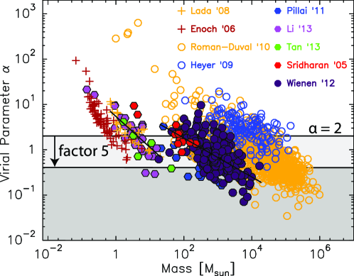
Figure 1.— The virial parameter, $\alpha$, as a function of fragment mass. Filled symbols indicate samples focusing on regions of high mass star formation (HMSF), while crosses indicate studies dealing with non–HMSF regions. Open circles are used for mixed samples that include clouds with and without HMSF. The horizontal black line at $\alpha=2$ gives the lowest critical virial parameter expected for non–magnetized clouds: fragments with $\alpha<2$ are supercritical and unstable to collapse, unless they are supported by significant magnetic fields. For reference, a virial parameter lower by a factor 5 is indicated using an arrow and another horizontal line. To illustrate power–law trends in virial parameters, fits to the Lada et al. (2008) and Wienen et al. (2012) samples are drawn using black lines.

3. Sample Selection & Data Analysis

This section explains how $\alpha$ is calculated from the data. The results are shown in Fig. 1. We compile a catalogue containing a total of 1325 virial parameter estimates for entire molecular clouds ($\gg{}1~{}\rm{}pc$ scale), clumps ($\sim{}1~{}\rm{}pc$), and cores ($\ll{}1~{}\rm{}pc$) with and without high mass star formation (HMSF).

As we detail below, observations of entire clouds are taken from Heyer et al. (2009) and Roman-Duval et al. (2010). Data for HMSF regions are from Sridharan et al. (2005), Pillai et al. (2011), Wienen et al. (2012), Li et al. (2013), and Tan et al. (2013). These samples all focus on, or exclusively study, early stages of HMSF. This means no or only faint sources are embedded in the fragments. We choose to concentrate on such young sources, because the state of more evolved objects is not necessarily representative of the initial conditions for star formation. For this reason, we do not include data from HMSF samples where—as discussed by the respective authors—evolutionary indicators like masers, mid–infrared emission, outflows, infall line profiles, etc., imply active star formation (Plume et al., 1997; Molinari et al., 2000; Beuther et al., 2002; Beltran et al., 2004; Fontani et al., 2005; Bontemps et al., 2010; Csengeri et al., 2011). Data for non–HMSF cores include cores in the Pipe Nebula (Lada et al., 2008) and Perseus molecular cloud (Enoch et al., 2006). Notes on individual samples are given in Sec. 3.2. Table 1 presents an overview over the different studies used here.

Our combined sample is not meant to be complete and unbiased; while our guiding principle is to provide a comprehensive overview, when possible we focus on larger samples that can easily be processed in the standardized way outlined below. A key aspect is that we only employ masses derived from observations of dust emission and extinction, and use a common set of dust opacities to derive masses from these data. This approach is chosen since mass measurements based on molecular line emission suffer from uncertainties due to unknown molecular abundances and excitation conditions. We deviate from this strategy only when considering very large clouds, for which only observations of molecular line emission from CO are available. Definitions of radius and velocity dispersion are standardized for all data, as explained below.

3.1. Data Processing

Several properties must be calculated to estimate the virial parameter. This is done as follows.

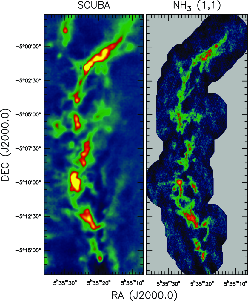
Figure 2.— Comparison of emission from dust (left panel; SCUBA data from Nutter & Ward-Thompson 2007) and Ammonia (middle; combined VLA and GBT data from Li et al. 2013). The correlation between the tracers is obvious. This justifies the use of tracers like Ammonia to characterize the kinematics of material detected in dust emission.

Velocity Dispersion, $\sigma_{v}$

Some studies provide the FWHM line width (Roman-Duval et al. 2010, Wienen et al. 2012, Bontemps et al. 2010, Pillai et al. 2011, Sridharan et al. 2005). In those cases, we calculate the corresponding velocity dispersion for a Gaussian line shape. We have discarded data where more than one velocity component is reported. This avoids the arbitrary choice of how the mass has to be divided up between the different velocity components.

The velocity dispersion $\sigma_{v}$ entering the calculation of the virial parameter reflects the combination of non–thermal gas motions, $\sigma_{v,\rm{}nt}$, and of the thermal motions of the particle of mean mass. The latter mass is $\langle{}m\rangle{}=2.33\,m_{\rm{}H}$ for molecular gas at the typical interstellar abundance of H, He, and metals (Appendix A of Kauffmann et al. 2008). For a molecule of mass $m$, the thermal velocity dispersion at temperature $T$ is $\sigma_{{\rm{}th},m}=288~{}{\rm{}m\,s^{-1}}\cdot{}(m/m_{\rm{}H})^{-1/2}\cdot{}(T/{10~{}\rm{}K})^{1/2}$, where $m_{\rm{}H}$ is the hydrogen mass. We combine these relations to estimate the dynamically relevant velocity dispersion as $\sigma^{2}_{v}=\sigma^{2}_{{\rm{}th},\langle{}m\rangle}+\sigma^{2}_{v,\rm{}nt}$. Similarly, the velocity dispersion observed for a molecule of mass $m$ is a combination of thermal and non–thermal gas motions, $\sigma^{2}_{v,\rm{}obs}=\sigma^{2}_{{\rm{}th},m}+\sigma^{2}_{v,\rm{}nt}$. We use the latter relation to estimate $\sigma_{v,\rm{}nt}$, which is then used to derive $\sigma_{v}$.

We have consistently used molecular emission lines selectively tracing dense gas to estimate velocity dispersions. This assures that the mass derived from dust emission, and the velocity dispersion from emission lines, probe the same volume. The dense gas tracers include $\mathrm{NH_{3}}$, $\mathrm{NH_{2}D}$, $\mathrm{N_{2}H^{+}}$, and $\mathrm{N_{2}D^{+}}$, and are not affected by depletion. Figure 2 illustrates the strong correlation between these tracers and the dust emission relevant for mass measurements. Tracers of lower density gas are only used for the two $\rm{}^{13}CO$–based cloud samples for which dust continuum data are not available (Heyer et al., 2009; Roman-Duval et al., 2010). In those cases, we have used $\rm{}^{13}CO$–derived masses and we have correspondingly derived $\alpha$ using $\rm{}^{13}CO$ velocity dispersions.

Radius, $R$

We adopt a common definition for the radius across all samples. Specifically, we determine the source area, $A$, and convert this into an effective radius, $R=(A/\pi)^{1/2}$. Some samples report an area contained in a specific contour, or they use other means to draw a clear outer source boundary. Other publications report the full width at half maximum (FWHM), and we use the FWHM area to determine $R$. As described below, we assure that mass and radius are consistent and refer to the same area.

Mass from Dust Emission, $M$

Most masses are estimated from dust emission. These masses are calculated from the observed flux following the formalism from Kauffmann et al. (2008),

$$\begin{array}[]{l}M=\displaystyle 0.12\,M_{\odot}\left({\rm e}^{1.439(\lambda/{\rm mm})^{-1}(T/{\rm 10~{}K})^{-1}}-1\right)\\ \quad\displaystyle\cdot\left(\frac{\kappa_{\nu}}{0.01\rm~{}cm^{2}~{}g^{-1}}\right)^{-1}\left(\frac{F_{\nu}}{\rm Jy}\right)\left(\frac{d}{\rm 100~{}pc}\right)^{2}\left(\frac{\lambda}{\rm mm}\right)^{3}\end{array}$$ (7)

where $\kappa_{\nu}$ is the dust opacity, and $F_{\nu}$ is the integrated flux for an object at distance $d$ and dust temperature $T$. We adopt a common opacity law $\kappa_{\nu}$ for dust grains with thin ice mantles coagulating for $10^{5}~{}\rm{}yr$ at density of $10^{6}~{}\rm{}cm^{-3}$ from Ossenkopf & Henning (1994). We adopt a gas–to–dust ratio of 100. We have used a power–law slope of 1.75 (Battersby et al., 2011) when interpolating and extrapolating (for wavelengths $\lambda>1.3~{}\rm{}mm$) between tabulated values.

As mentioned before, we assure that mass and radius are consistent and refer to the same area. Most publications report the flux for the aforementioned area $A$ used to derive the effective radius. A different approach is taken by Wienen et al. (2012) and Sridharan et al. (2005): these authors report FWHM sizes (Sridharan et al. take those data from Beuther et al. 2002), while the reported fluxes are integrated over a full Gaussian model fitted to sources. The latter model exceeds the spatial extent of the FWHM area. To derive mass and size estimates for the same area, the mass—respectively the observed flux—is reduced by a factor 0.69 (see Kauffmann & Pillai 2010).

Mass from Dust Extinction, $M$

Core masses in the Pipe nebula are based on extinction data of Alves et al. (2007). They use the NICER method on the data from 2MASS bands ($1.25~{}\mu\rm{}m$, $1.65~{}\mu\rm{}m$, $2.2~{}\mu\mbox{m}$). Core masses are obtained using an extinction law $A_{K}/A_{V}=0.112$ and a conversion factor from extinction to column density of $N({\rm{}H_{2}})/A_{V}=9.4\times{}10^{20}~{}\rm{}cm^{-2}\,mag^{-1}$. As shown in Kauffmann et al. (2010a), based on work by Bianchi et al. (2003), such extinction–based masses are within a factor $\sim{}1.5$ consistent with masses derived from dust emission using the aforementioned formalism.

Mass from ¹³CO Emission, $M$

The $\rm{}^{13}CO$–based masses are taken directly from the original publications. These latter mass measurements are not standardized with respect to the dust observations and they suffer from other and larger uncertainties (e.g., in abundance). Also, the interpretation of virial parameters depends on how exactly the observed $\rm{}^{13}CO$ luminosity traces a cloud’s mass reservoir (e.g., Maloney 1990). Here, $\rm{}^{13}CO$–based masses are shown for completeness; they are not used in our main analysis.

Virial Parameter, $\alpha$

From the properties derived above, the virial parameter $\alpha$ is eventually calculated in the same way for all cloud fragments using Eq. (1).

Observational Uncertainties

The aforementioned observational properties suffer from a variety of observational uncertainties. Because of the flow of the argument, it is most useful to discuss these uncertainties in the context of the physical interpretation of the results. This is done at the end of this document in Sec. 6. We briefly note that the expected mass uncertainties are of order of a factor 2, and are the largest uncertainty in calculating $\alpha$. The resulting virial parameters are uncertain by a similar factor.

3.2. Individual Samples

Giant Molecular Clouds

We have used data from the $\rm{}^{13}CO$–based survey of giant molecular clouds (GMCs) by Roman-Duval et al. (2010). They derive masses, sizes and kinematics for 750 molecular clouds based on the Boston University–Five College Radio Astronomy Observatory (BU–FCRAO) Galactic Ring Survey (GRS). This data has overlap with the GRS data published for 162 GMCs of Heyer et al. (2009). We also plot the latter sample for consistency. Note that these data are the only ones for which we have used gas masses estimated from molecular line emission. They are estimated from ${}^{13}\rm{CO}$ data assuming an excitation temperature from the ${}^{12}\rm{CO}$ line emission and a CO–to–$\rm{}H_{2}$ abundance ratio of $8\times{}10^{-5}$. The studies further assume that the ${}^{12}\rm{CO}$–to–${}^{13}\rm{CO}$ abundance varies with galactocentric radius as described by Frerking et al. (1982), respectively Milam et al. (2005), depending on the study. We stress that the $\rm{}^{13}CO$–based data are shown for completeness, but that they suffer from other biases than the dust–based observations that are the focus of this study. To calculate the thermal velocity dispersion, a common gas temperature of $10~{}\rm{}K$ is assumed for all clouds in these samples.

HMSF Clumps

We have compiled published data from Wienen et al. (2012), who present a comprehensive catalog of cold (hence likely prestellar) high mass clumps identified from an unbiased continuum survey of the inner Galactic Plane at $870~{}\rm{}\mu{}m$. Masses are determined from the latter data. We use their $\rm{}NH_{3}$ (1,1) Effelsberg 100m–telescope data to obtain velocity dispersions and estimate dust temperatures for mass measurements. This allows to determine $\alpha$ for 260 clumps with well–known distances: these clouds were either at tangential points, or the distance ambiguity was previously resolved by Roman-Duval et al. (2010) on the basis of $21~{}\rm{}cm$ observations of Hi.

non–HMSF Cores

Results on Perseus and the Pipe Nebula represent non–HMSF clouds. We have included masses from near–infrared extinction data (Lada et al., 2008) and kinematics from GBT $\rm{}NH_{3}$ (1,1) data (Rathborne et al., 2008) for 29 cores in the Pipe Nebula. The temperature is fixed to the average $\rm{}NH_{3}$–based temperature of $10~{}\rm{}K$. In Perseus, we have combined masses from Bolocam dust continuum data (Enoch et al., 2006) with gas temperatures and velocity dispersions gleaned from GBT $\rm{}NH_{3}$ (1,1) data (Rosolowsky et al., 2008). Enoch et al. provide the integrated flux density for several apertures. We chose to adopt an aperture size of $40\arcsec$ to derive mass estimates, since it closely matches the GBT $\mathrm{NH_{3}}$ beam.

HMSF Cores

Since HMSF clouds are typically more distant than non–HMSF regions, interferometer observations are required to achieve a spatial resolution similar to the one of observations of low mass cores. We thus compile a large sample of high resolution observations of potential prestellar stages of high mass star formation. For the quiescent cores in Orion, we have calculated $\alpha$ combining gas kinematics and temperatures from the VLA $\rm{}NH_{3}$ (1,1) data of Li et al. (2013) with mass estimates from SCUBA $850~{}\rm\mu{}m$ observations by Nutter & Ward-Thompson (2007). We have estimated $\alpha$ for the high mass cores identified in G29.96$-$0.02 and W48 HMSF regions studied by Pillai et al. (2011). For this, we used the 3 mm dust continuum cores with associated $\mathrm{NH_{2}D}$ 1₁₁–1₀₁ emission, and used these tracers to determine masses and kinematics, respectively. The temperature is fixed to the average $\rm{}NH_{3}$–based temperature of $16~{}\rm{}K$. To characterize the Sridharan et al. (2005) sample, we glean gas kinematics and estimated dust temperatures from the $\rm{}NH_{3}$ data presented by Sridharan et al., and then estimate masses from dust emission observations first reported by Beuther et al. (2002). Data from a recent ALMA study of high mass cores by Tan et al. (2013) are also included. We used emission from dust and $\rm{}N_{2}D^{+}$ to constrain masses and gas motions. Since Tan et al. use a different gas–to–dust ratio than us (i.e., 147 vs. our value of 100), we recompute the mass (given in their Table 3) for the same gas–to–dust ratio as we have adopted in this work. We follow Tan et al. in assuming dust and gas temperatures of $10~{}\rm{}K$.

Table 1Data Summary

Sample	$\langle R\rangle$	sample mediana $\langle\Sigma_{M}\rangle$	SF Modeb	$\sigma_{v}$ from	total mass from
	pc	$\mathrm{g\,cm^{-2}}$
Enoch et al.	0.02	0.04	non–HMSF	$\mathrm{NH_{3}}$ (1,1)	1100 µm
Heyer et al.	3.91	0.04	undetermined	$\mathrm{{}^{13}CO}$ (1–0)	$\mathrm{{}^{13}CO}$ (1–0)
Lada et al.	0.12	0.01	non-HMSF	$\mathrm{NH_{3}}$ (1,1)	NIR extinction
Li et al.	0.04	0.18	HMSF	$\mathrm{NH_{3}}$ (1,1)	850µm
Pillai et al.	0.29	0.12	HMSF	$\mathrm{NH_{2}D}$ (111–101)	3500 µm
Roman–Duval et al.	8.33	0.03	undetermined	$\mathrm{{}^{13}CO}$ (1–0)	$\mathrm{{}^{13}CO}$ (1–0)
Sridharan et al.	0.22	0.10	HMSF	$\mathrm{NH_{3}}$ (1,1)	1200µm
Tan et al.	0.06	0.13	HMSF	$\mathrm{N_{2}D^{+}}$ (3–2)	1338µm
Wienen et al.	0.68	0.15	HMSF	$\mathrm{NH_{3}}$ (1,1)	870µm

^athe median value of $\langle\Sigma_{M}\rangle$ determined for a given sample

^bmode of star formation (i.e., high–mass stars are present or not, or should form in future), as judged by the original authors; for “undetermined” samples, the star formation modes of the clouds have not been assessed, but are likely mixed

4. Observed Trends in Virial Parameters

4.1. Observed Trends

As seen in Figure 1, all of the data presented here follow a number of common trends. Most fundamentally, within a given sample, all data follow a power–law

$$\alpha=\alpha_{0}\cdot{}(M/10^{3}\,M_{\sun})^{h_{\alpha}}$$ (8)

with a similar slope, $h_{\alpha}$, and a range of intercepts, $\alpha_{0}$. This power–law behavior has already been noticed by BM and also reported by, e.g., Lada et al. (2008) and Foster et al. (2009). To illustrate these trends, fits to the Lada et al. (2008) and Wienen et al. (2012) samples are drawn into Fig. 1.

The sequences formed by a given sample terminate at a maximum mass, $M_{\rm{}max}$, corresponding to a minimum virial parameter, $\alpha_{\rm{}min}$. This is remarkable, since larger masses—and therefore lower virial parameters—would be easily detected, if present. By contrast, sequence terminations at lower mass cannot be determined due to limited mass sensitivities. To highlight this trend, one may rewrite Eq. (8) as

$$\alpha=\alpha_{\rm{}min}\cdot{}(M/M_{\rm{}max})^{h_{\alpha}}\,{},$$ (9)

where $\alpha_{0}=\alpha_{\rm{}min}\cdot{}(M_{\rm{}max}/10^{3}\,M_{\sun})^{-h_{\alpha}}$. Table 2 summarizes the power–laws representing the various samples. To gauge the accuracy of these fits, the table also lists the root mean square (RMS) deviation between the logarithms of the actual observations and the fit, $\delta_{\log_{10}(\alpha)}=\langle{}[\log_{10}(\alpha_{i})-\log_{10}(\alpha(M_{i}))]^{2}\rangle^{1/2}$.

Table 2Virial Parameter Power Laws

Sample	$\alpha_{0}$	$\alpha_{\rm{}min}$	$M_{\rm{}max}/M_{\sun}$	$h_{\alpha}$	$\delta_{\log_{10}(\alpha)}$
Enoch et al.	0.00	0.33	6	$-$0.99	0.19
Heyer et al.	3.11	1.71	$1.4\times{}10^{5}$	$-$0.12	0.30
Lada et al.	0.05	0.65	20	$-$0.68	0.15
Li et al.	0.02	0.64	16	$-$0.79	0.21
Pillai et al.	0.17	0.15	$1.3\times{}10^{3}$	$-$0.61	0.19
Roman–Duval	2.00	0.16	$1.0\times{}10^{6}$	$-$0.37	0.33
et al.
Sridharan	0.55	1.11	226	$-$0.47	0.13
et al.
Tan et al.	0.06	0.39	43	$-$0.62	0.17
Wienen et al.	0.68	0.20	$1.9\times{}10^{4}$	$-$0.43	0.27

While some trends are similar for all samples, others differ among the various studies.

1. When considering objects of increasing mass, all samples terminate at a maximum mass and minimum virial parameter, $M_{\rm{}max}$ and $\alpha_{\rm{}min}$. Values $\alpha_{\rm{}min}\ll{}2$ are observed for a number of samples. Some observations for individual fragments are even below the $\alpha_{\rm{}min}$ derived from fits to the samples.

2. All samples have very similar $\alpha(M)$ slopes, $h_{\alpha}$, observed to be in the range $0<-h_{\alpha}<1$.

3. The samples do significantly differ in their intercepts, $\alpha_{0}$. Differences by more than an order of magnitude are observed.

Note that the observed anti–correlation between mass and virial parameter is not a consequence of an unfortunate combination of errors in mass estimates and the inherent relation $\alpha{}\propto{}M^{-1}$. Uncertainties in mass estimates are of order of a factor 2 (Sec. 6.2), while all samples span more than an order of magnitude in mass. Errors in mass estimates can therefore not significantly affect the observed correlations.

4.2. Virial Parameter Slope

The trends in virial parameter slope and intercept result from the slopes of the well–known mass–size and linewidth–size relations for molecular clouds. To show this, we express the virial parameter slope as $\,{\rm{}d}{}\log(\alpha)/\,{\rm{}d}{}\log(M)$, the mass–size slope as $\,{\rm{}d}{}\log(M)/\,{\rm{}d}{}\log(R)$, and the linewidth–size relation as $\,{\rm{}d}{}\log(\sigma_{v})/\,{\rm{}d}{}\log(R)$. Logarithmic differentiation of the definition of the virial parameter (Eq. 1a) yields

$$\frac{\,{\rm{}d}\log(\alpha)}{\,{\rm{}d}\log(M)}=\frac{2\frac{\,{\rm{}d}\log(\sigma_{v})}{\,{\rm{}d}\log(R)}+1-\frac{\,{\rm{}d}\log(M)}{\,{\rm{}d}\log(R)}}{\frac{\,{\rm{}d}{}\log(M)}{\,{\rm{}d}{}\log(R)}}$$ (10)

(see Appendix B4). This demonstrates that the various slopes directly depend on another. In practice, as seen in Table 2, the virial parameter slope varies little between the various samples. Following Eq. (10), this is a consequence of how mass–size and linewidth–size laws combine in individual samples.

To explore this a bit more, Fig. 3 shows the connections between velocity dispersion, radius, and mass. This representation suggests that the cloud fragments in a given sample obey common mass–size and linewidth–size relations described by power–laws (note that we investigate trends for the non–thermal velocity dispersion, $\sigma_{v,{\rm{}nt}}$),

$$M=M_{0}\cdot{}(R/{\rm{}pc})^{h_{M}}\quad{\rm{}and}$$ (11)

$$\sigma_{v,\rm{}nt}=\sigma_{v,0}\cdot{}(R/{\rm{}pc})^{h_{\sigma_{v}}}\,{}.$$ (12)

Table 3 lists fitted properties for the various samples. To indicate trends, the fits for the Lada et al. (2008) and Wienen et al. (2012) samples are indicated in Fig. 3.

For linewidth–size laws, we experiment with assuming a common slope of $h_{\sigma_{v}}=0.32$. This is the slope derived when fitting all data with a common relation. The fit gives an intercept $\sigma_{v,0}=0.8~{}\rm{}km\,s^{-1}$. The RMS deviation between fit and observations is $\delta_{\log_{10}(\sigma_{v})}=\langle{}[\log_{10}(\sigma_{v,i}/\sigma_{v}(R_{i}))]^{2}\rangle^{1/2}=0.24$, i.e., the RMS scatter is of the order of a factor $10^{0.24}=1.7$. When we use $h_{\sigma_{v}}=0.32$ to fit individual samples, the fit results and deviations given in Table 3 are obtained. For all but one sample, we find good fits characterized by $\delta_{\log_{10}(\sigma_{v})}<0.2$, i.e., an RMS scatter of a factor $<1.6$. For the Lada et al. (2008) study, $\delta_{\log_{10}(\sigma_{v})}=0.35$, equivalent to a factor $10^{0.35}=2.2$, is obtained. As already noted by Lada et al., the latter probably reflects the fact that the dense cores in the Pipe Nebula are “coherent” (Barranco & Goodman 1998, Goodman et al. 1998), i.e., thermal motions play a significant or dominant role. The residual non–thermal motions are often negligible, and they do not closely obey linewidth–size laws. With the exception of the Lada et al. sample, the derived intercepts are within a factor 2 from the intercept derived for a common fit to all data, $\sigma_{v,0}=0.8~{}\rm{}km\,s^{-1}$.

This shows that the mass–size and linewidth–size laws are indeed relatively similar for all samples. One could now use the approximations $\,{\rm{}d}{}\log(M)/\,{\rm{}d}{}\log(R)\approx{}h_{M}$ and $\,{\rm{}d}{}\log(\sigma_{v})/\,{\rm{}d}{}\log(R)\approx{}h_{\sigma_{v}}$ to derive $h_{\alpha}$ as $\,{\rm{}d}{}\log(\alpha)/\,{\rm{}d}{}\log(M)$ via Eq. (10). In practice, though, this is an exercise of limited value, given the approximations involved. In any case, as shown by Eq. (10), the slopes depend on another.

We note that a virial parameter slope $h_{\alpha}=-2/3$ has previously been predicted by BM. For example, Lada et al. (2008) interpret their data in BM’s framework. Specifically, a value $h_{\alpha}=-2/3$ is expected if all fragments in a sample have the same mean density and the same velocity dispersion. To see this, one may use the mean density $\langle{}\varrho{}\rangle=M/(4/3\,\pi\,R^{3})$ to rewrite the virial parameter as $\alpha=C\cdot{}\sigma_{v}^{2}\,M^{-2/3}\,\langle{}\varrho{}\rangle^{-1/3}$, where $C$ is a numerical constant. This implies $\alpha\propto{}M^{-2/3}$, and thus $h_{\alpha}=-2/3$, if $\sigma_{v}$ and $\langle{}\varrho{}\rangle$ are constant. BM highlight that $\langle{}\varrho{}\rangle$ is indeed constant in samples of pressure–confined fragments—i.e., where self–gravity is negligible—that are subject to the same confining pressure and have a common $\sigma_{v}$. Many of the slopes noted in Table 2 are about consistent with $h_{\alpha}=-2/3$ and fulfil this prediction for pressure–confined fragments. Note, however, that self–gravity plays a significant role in most of the samples, as indicated by values of $\alpha_{\rm{}min}$ much below $\alpha_{\rm{}BE}$. The aforementioned theory predicting $h_{\alpha}=-2/3$, which only applies to fragments with negligible self–gravity, does thus not apply.

Table 3Mass–Size and Linewidth–Size Laws

Sample	$h_{M}$	$\sigma_{v,0}/\rm{}km\,s^{-1}$	$\delta_{\log_{10}(\sigma_{v})}$
Enoch et al.	—a	0.49	0.20
Heyer et al.	$1.40\pm{}0.07$	1.42	0.16
Lada et al.	$2.46\pm{}0.14$	0.20	0.35
Li et al.	$1.86\pm{}0.66$	0.85	0.18
Pillai et al.	$2.22\pm{}0.61$	0.69	0.15
Roman–Duval et al.	$2.36\pm{}0.02$	0.69	0.18
Sridharan et al.	$1.80\pm{}0.23$	1.15	0.12
Tan et al.	$2.96\pm{}0.95$	0.74	0.12
Wienen et al.	$1.77\pm{}0.07$	1.05	0.16

^ano trend with radius, since all observations are obtained for a fixed aperture

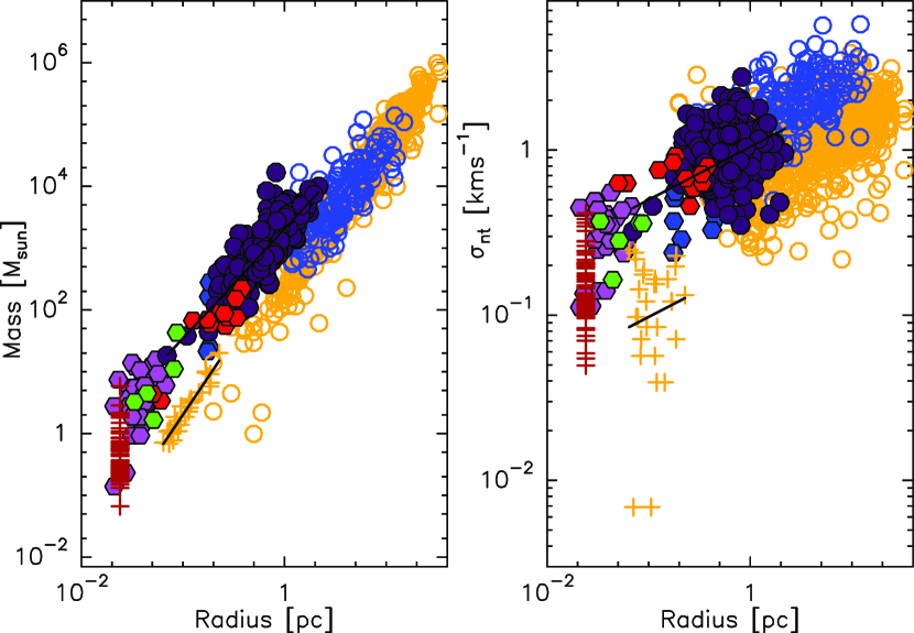
Figure 3.— Mass–size and linewidth–size trends in our catalogue. Colored symbols refer to the samples indicated in Fig. 1.

4.3. Virial Parameter Intercept

To explore the virial parameter intercepts, consider mean mass surface densities, $\langle{}\Sigma_{M}\rangle{}=M/(\pi{}R^{2})$. Substitution of the linewidth–size law in Eq. (1), plus replacing $R$ with $\langle{}\Sigma_{M}\rangle$ and $M$, yields

$$\begin{array}[]{l}\displaystyle\alpha=1.2\,\left(\frac{\sigma_{v}}{\sigma_{v,\rm{}nt}}\right)^{2}\\ \displaystyle\quad\quad\,\,\cdot\left(\frac{\sigma_{v,0}}{\rm{}km\,s^{-1}}\right)^{2}\frac{(M/10^{3}\,M_{\sun})^{h_{\sigma_{v}}-1/2}}{(\langle{}\Sigma_{M}\rangle{}/0.066~{}{\rm{}g\,cm^{-2}})^{h_{\sigma_{v}}+1/2}}\,,\end{array}$$ (13)

where we use that $1~{}{\rm{}g\,cm^{-2}}=4800\,M_{\sun}\,\rm{}pc^{-2}$. The factor $(\sigma_{v}/\sigma_{v,\rm{}nt})^{2}$ provides a correction in the case that non–thermal gas motions are important. Note that Eq. (13) does not present an approximation; for example, provided parameters for individual fragments are substituted, Fig. 1 could be constructed via Eq. (13) in all details.

This shows that the virial parameter intercept strongly depends on the linewidth–size intercept and the mean mass surface density of a sample. The latter varies dramatically between the samples, as seen in Table 1, largely due to the sensitivity of different observational methods. As in the case of Eq. (10), we abstain from attempt to substitute characteristic values for samples into Eq. (13). Experimentation shows that, e.g., $\sigma_{v,0}$ and $\langle{}\Sigma_{M}\rangle$ vary too strongly within samples to derive meaningful results.

4.4. Low Virial Parameters

To fully describe the observed virial parameter laws, we finally need to interpret the observed minimum virial parameters $\alpha_{\rm{}min}\ll{}2$. The remainder of the paper is dedicated to this.

5. Implications of Low Virial Parameters

Figure 1 and Table 2 show that the observed minimum virial parameters in many samples fall below the fiducial critical value $\alpha{}=2$ by a factor of 5 or more. This is a significant difference beyond the range expected from observational uncertainties, as we explore in Sec. 6. Given critical virial parameters $\alpha_{B=0}\gtrsim{}2$, fragments characterized by $\alpha{}\ll{}2$ must be unstable to collapse unless they are supported by significant magnetic fields. In this section, we discuss what this conclusion means for our understanding of the star formation process.

To make the discussion more readable, some of the quantitative details of the discussion have been removed to Appendix C. The current section focuses on the main implications from the analysis.

Note that the smallest virial parameters are found in regions of high mass star formation (HMSF). See for example Fig. 1, where HMSF regions are indicated by filled symbols. Specifically, the HMSF samples from Pillai et al. (2011), Li et al. (2013), Tan et al. (2013), and Wienen et al. (2012) contain virial parameters much smaller than those in the non–HMSF samples by Lada et al. (2008) and Enoch et al. (2006). Also Table 2 lists the smallest $\alpha_{\rm{}min}$ for HMSF sites. This is a consequence of the high mass of HMSF clouds, which are observed to exceed an approximate size–dependent threshold, $M(R)>M_{\rm{}HMSF}(R)$ where

$$M_{\rm{}HMSF}(R)=870\,M_{\sun}\,\left(\frac{\kappa(\nu)}{\kappa_{\rm{}OH}(\nu)/1.5}\right)^{-1}\left(\frac{R}{\rm{}pc}\right)^{1.33}$$ (14)

(Kauffmann & Pillai 2010; see yellow shading in Fig. 4). This relation depends on the adopted dust opacity law. A relation $\kappa(\nu)=\kappa_{\rm{}OH}(\nu)/1.5$ was adopted in the original work (Kauffmann et al. 2010a, b; Kauffmann & Pillai 2010). Equation (C1) demonstrates that $M(R)>M_{\rm{}HMSF}(R)$ implies $\alpha{}\lesssim{}1$ for radii $\sim{}0.1~{}\rm{}pc$.

In essence, the observed virial parameters are low because the observed velocity dispersions are low for the given mass and size of a fragment. To provide a reference, Fig. 4(a) illustrates the velocity dispersion needed to achieve $\alpha=2$.

5.1. Short Lifetimes of High–Mass Starless Cores

The study of high mass star formation is still trying to answer a central and important riddle: why are there no starless cores of high mass and density? The absence of such cores is significant, given that many starless cores exist in non–HMSF regions (see, e.g., Evans et al. 2009 for statistics). After the discovery of Infrared Dark Clouds (IRDCs), it has been speculated that some cores within these clouds would represent high mass starless cores (e.g., Egan et al. 1998, Carey et al. 1998). Follow–up studies do indeed show that IRDCs form high–mass stars (e.g., Beuther et al. 2005, Pillai et al. 2006, Rathborne et al. 2007). Such work also revealed potential high mass starless cores in IRDCs (e.g., Sridharan et al. 2005, Swift 2009 Pillai et al. 2011 Wienen et al. 2012, Tan et al. 2013). However, to our best knowledge, the few objects that were studied with targeted follow–up observations are not found to be clear–cut high–mass starless cores.

This implies that high–mass starless cores are rare. Such a trend further implies that the lifetime of such cores must be low. The low observed virial parameters might explain why this is the case.

Cloud fragments with virial parameters $\alpha{}\ll{}2$ might collapse very quickly, essentially in a free–fall time, if magnetic fields are insignificant for support against self–gravity. This follows from the fact that non–magnetized cloud fragments with virial parameters $\alpha{}\ll{}\alpha_{\rm{}BE}$ are not supported against gravitational collapse. In HMSF regions, mass and size are related by the approximate threshold for high–mass star formation, Eq. (14). When we substitute this relation into the equation for the free–fall timescale (Appendix C.2), we find that $\tau_{\rm{}ff}<5.5\times{}10^{4}~{}{\rm{}yr}\cdot{}(M/10\,M_{\sun})^{0.62}$ holds for cloud fragments $M>M_{\rm{}HMSF}$ deemed able to form high–mass stars. This implies short lifetimes for non–magnetized fragments, just as needed to explain the absence of high–mass starless cores.

5.2. “Turbulent Core Accretion” in HMSF

High–mass star formation requires high accretion rates onto the stars. For example, in Pillai et al. (2011) we summarize previous work suggesting that accretion rates $\geq{}10^{-4}\,M_{\sun}\,\rm{}yr^{-1}$ are needed to form stars of a mass $\geq{}10\,M_{\sun}$ during the estimated duration of the accretion phase $\leq{}10^{5}~{}\rm{}yr$. Accretion rates of this order are, for example, expected for the collapse of spheres that were initially in hydrostatic equilibrium and supported by sufficiently fast random gas motions. In non–magnetized spheres, stellar accretion rates $\dot{M}_{\star}\leq{}2.3\times{}10^{-4}\,M_{\sun}\,{\rm{}yr}\cdot{}(\sigma_{v}/{\rm{}km\,s^{-1}})^{3}$ are then possible (Shu, 1977; McKee & Tan, 2002, 2003; Pillai et al., 2011). The non–magnetized version of the “turbulent core” HMSF model by McKee & Tan (2002, 2003) posits that high accretion rates in HMSF do indeed result from the collapse of cloud fragments initially supported by high velocity dispersions. However, there are issues with this picture.

For example, as we show throughout this paper, many HMSF cloud fragments have virial parameters much below the critical value for non–magnetized media. This means that many HMSF fragments are not in hydrostatic equilibrium, and so the original model from McKee & Tan (2002) does not apply, as it requires $\alpha{}\gtrsim{}2$. This problem is also noted by Tan et al. (2013). They suggest to include additional support from magnetic fields. This would, however, reduce the role of $\sigma_{v}$ and represent a major modification of the initial McKee & Tan (2002) model. Such refinements are explored by McKee & Tan (2003). In this more complete picture, the velocity dispersion $\sigma_{v}$ is not the only factor controlling $\dot{M}_{\star}$.

Another issue is that, for the non–magnetized case, the substitution of observed velocity dispersions yields accretion rates only marginally consistent with $\dot{M}_{\star}\geq{}10^{-4}\,M_{\sun}\,\rm{}yr^{-1}$ (Pillai et al., 2011). If magnetic fields are present, the model accretion rates would be higher by a factor 6.6 when adopting the fiducial magnetic field properties proposed by McKee & Tan (2003; their $H_{0}=1$ and $\phi_{B}=2.8$).

5.3. Competitive Accretion

It is currently not clear by which accretion mechanism high–mass stars grow in mass. One theory posits that individual dense cores produce individual stars or close binaries. Here, we refer to this process as “monolithic accretion” (Zinnecker & Yorke 2007; e.g., the McKee & Tan 2002, 2003 models belong to this category). Alternative theories propose that no well–defined HMSF dense cores exist. In this scenario of “competitive accretion”, several stars vie with another to accrete from a common gas reservoir. This star formation mechanism has been studied by, e.g., Bonnell et al. (1997, 2001a, 2001b) and Bate & Bonnell (2005).

Krumholz et al. (2005) show that competitive accretion requires virial parameters $<1$. This follows from the constraints that competitive accretion works best if the gas densities are high and the relative velocity between star and gas are small, and can be evaluated for the case of Bondy–Hoyle accretion. In their original work, Krumholz et al. (2005) compiled virial parameters from a small sample of clouds and clumps. Those data suggested that $\alpha{}\gtrsim{}1$. Krumholz et al. interpreted this as evidence that competitive accretion is not possible in HMSF regions.

The larger sample depicted in Fig. 1, however, shows that $\alpha{}<1$ is frequently observed in regions of high mass star formation. This new result demonstrates that competitive accretion would be possible in many of the clouds studied here. Note that this does not, however, constitute evidence against monolithic accretion. We also caution that some of the fragments with $\alpha<1$ might not be massive enough to form entire clusters. In that case, competitive accretion cannot operate, since it requires the presence of a significant cluster. Figure 4(b) illustrates the mass–size domain in which $\alpha<1$, so that competitive accretion becomes possible.

Note, further, that Krumholz et al. (2005) propose the additional limit that competitive accretion requires $\alpha^{2}\,M\lesssim{}10\,M_{\sun}$. The exact value of this threshold depends on model details (Krumholz et al., 2005), and it may be larger than the fiducial value by an order of magnitude (Bonnell & Bate, 2006). When selecting fragments with $M(R)>M_{\rm{}HMSF}(R)$ from the HMSF samples, 6 objects fulfil $\alpha^{2}\,M<10\,M_{\sun}$.

5.4. Fragments with Small Virial Parameters
are not Collapsing

By definition, $\alpha<\alpha_{\rm{}cr}$ implies that a cloud fragment is susceptible to collapse. Thus, it has often been argued that cloud fragments with virial parameters $\alpha\ll{}\alpha_{\rm{}BE}\approx{}2$ are indeed collapsing to form a star. However, this is a flawed argument: provided energy is conserved, fragments well into collapse contain gas rapidly moving inward, and velocity dispersions obtained under these conditions imply virial parameters $\approx{}2a=4\pm{}2$ (see Appendix C.3), since $a=2\pm{}1$. As a consequence, fragments with $\alpha\ll{}\alpha_{\rm{}BE}\approx{}2$ are not likely to be in a state of collapse. This has previously been realized by, for example, Larson (1981) and Ballesteros-Paredes (2006).

One important caveat is that this argument assumes conservation of energy. This is a reasonable ansatz. To circumvent this constraint, energy would need to be drained from the system at a very high rate. Doing so is not a trivial problem (see Appendix C.3 for some example calculations).

It thus appears plausible that fragments with virial parameters $\ll{}2$ are not collapsing. Fragments in this state would then need to be supported by additional forces. Alternatively, they might be short–lived and soon collapse in a free–fall time (Sec. 5.1).

5.5. Evidence for Significant Magnetic Fields?

Let us assume that cloud fragments with $\alpha\ll{}2$ are indeed not undergoing collapse, as argued in Sec. 5.4. The most straightforward explanation for such fragments would be that they are supported against collapse by significant magnetic fields.

Equation (6) gives the critical virial parameter in this situation. This relation only depends on $M_{\Phi}/M_{\rm{}BE}$, which essentially measures the relative importance of support from magnetic fields relative to random gas motions. If we require that $\alpha\geq{}\alpha_{\rm{}cr,\Phi}$, we can rewrite Eq. (6) to obtain

$$\frac{M_{\Phi}}{M_{\rm{}BE}}\gtrsim\frac{2}{\alpha}-1\,.$$ (15)

Combination of Eqs. (3, 5) permits us to estimate the magnetic field strength as

$$B=81~{}{\rm{}\mu{}G}\,\frac{M_{\Phi}}{M_{\rm{}BE}}\,\left(\frac{\sigma_{v}}{\rm{}km\,s^{-1}}\right)^{2}\left(\frac{R}{\rm{}pc}\right)^{-1}\,.$$ (16)

For example, the lowest observed virial parameters are of order 0.2. This implies mass ratios $M_{\Phi}/M_{\rm{}BE}\approx{}10$. Those cloud fragments are also observed to have velocity dispersions $\sim{}0.5~{}\rm{}km\,s^{-1}$, radii $\sim{}0.1~{}\rm{}pc$, and masses $\sim{}10^{2}\,M_{\sun}$. Following Eq. (16), this implies field strengths $\sim{}2~{}\rm{}mG$. This is a very high value. However, it is marginally in the range expected for cloud fragments of very high density. Crutcher (2012) suggests an approximate density–dependent upper limit to the magnetic field strength (Appendix C.4). Substitution of the aforementioned masses and sizes gives field strengths $B\lesssim{}1.5~{}\rm{}mG$, marginally consistent with the above estimate $\sim{}2~{}\rm{}mG$.

Representative values for the maximum critical mass of magnetized clouds, $M_{B}\lesssim{}M_{\rm{}BE}+M_{\Phi}$, are given in Fig. 4(c). All cloud fragments below the $B=0$ curve are subcritical even if not supported by magnetic fields.

5.6. Mass Estimates from Virial Analysis

In the absence of better tracers, the virial mass $M_{\rm{}vir}\equiv 5\sigma_{v}^{2}R/G$ is often used to estimate the true mass, $M$. Basically, this assumes that $M\approx{}M_{\rm{}vir}$. Since $\alpha{}\equiv{}M_{\rm{}vir}/M$ by definition, this requires that $\alpha{}\approx{}1$. Figure 1 shows that, for individual cloud fragments, this assumption is violated by factors 10 and more: in this case, the mass estimated via a virial analysis is off by the same factor. For individual objects, this large uncertainty must be kept in mind when using masses estimated in this fashion.

That said, it might be appropriate to determine, e.g., the total gas mass contained in a cloud sample via a virial analysis. As seen in Fig. 1, the scatter is large for individual objects, but the average virial parameter is often well defined for a given sample, and is often observed to be of order unity. A careful analysis of cloud samples could exploit such trends.

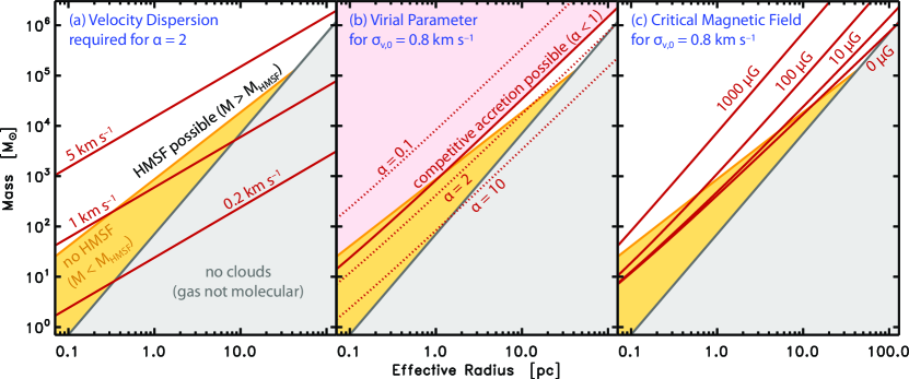
Figure 4.— Implications for star–formation physics. Yellow shading highlights the region in which cloud fragments are not massive enough to host high mass star formation (HMSF). The limit drawn in this figure is taken from Kauffmann & Pillai (2010) and assumes—in contrast to all other parts of the paper—a dust opacity $\kappa(\nu)=\kappa_{\rm{}OH}(\nu)/1.5$. Red lines in panel (a) give the minimum velocity dispersion needed to render a non–magnetized cloud fragment stable against gravitational collapse ($\alpha=2$). Panel (b) presents estimated virial parameters as a function of mass and size, as expected for $15~{}\rm{}K$ gas temperature and a common linewidth–size law with $h_{\sigma_{v}}=0.32$ and $\sigma_{v,0}=0.8~{}\rm{}km\,s^{-1}$. Red shading indicates where competitive accretion is expected to be possible ($\alpha<1$). In panel (c) the same temperature and linewidth–size law is assumed to estimate the minimum “critical” magnetic field strength needed to render a cloud fragment stable against gravitational collapse. The grey shading indicates cloud fragments with a mean visual extinction $A_{V}<1~{}\rm{}mag$. That part of the parameter space is devoid of molecular clouds, since the mean visual extinction is too low to shield the molecular gas from photodissociation.

6. Virial Parameters: Impact of Uncertainties

The analysis above builds on various assumptions to calculate $\alpha$ and $\alpha_{\rm{}cr}$. Here we explore whether uncertainties in these assumptions might affect our conclusions.

6.1. Observational Approaches

The way in which properties are calculated can significantly affect the results. This is seen in Fig. 1, where the results do significantly differ between Heyer et al. (2009) and Roman-Duval et al. (2010), although both studies build on the same set of observations. The difference lies in the way cloud structure was extracted: Heyer et al. examine boxes drawn around clouds, which serves their purpose but is not ideal to measure $\alpha$, while Roman-Duval et al. closely follow the cloud shape and derive properties better suited for a virial analysis. This example demonstrates that determining the virial parameter is a difficult task.

6.2. Errors in Mass Estimates

The most commonly adopted dust model for cold dense cores, which is also used in this paper, has been forwarded by Ossenkopf & Henning (1994). The resulting opacity is intermediate to the values proposed by, e.g., Krügel & Siebenmorgen (1994) and Motte et al. (1998), who forward values higher or lower by a factor 2. If we confine ourselves to the range in these models, even if the true dust opacities were higher, that would account for only a systematic uncertainty of a factor 2 in dust masses and therefore virial parameters. An error in the opacity by a factor $>10$, as needed to render fragments with estimated $\alpha{}=0.2$ subcritical, seems implausible.

The mass is approximately inversely proportional to the adopted dust temperature. For some objects in our analysis, dust temperatures were estimated by assuming that they are similar to gas temperatures. For example, using observations of $\rm{}NH_{3}$, Rathborne et al. (2008) derive temperatures for the sample of Lada et al. (2008), and Li et al. (2013) obtain own data for their sample. For starless cores, such work typically finds temperatures in the range 10–15$~{}\rm{}K$. Direct estimates of dust temperatures from continuum emission yield similar values for regions not in the immediate vicinity of HMSF (e.g., Hill et al. 2011). Following Kauffmann et al. (2008), the conversion factor between dust emission and mass varies by a factor $\leq{}1.75$ for dust temperatures in the range 10–15$~{}\rm{}K$ and dust emission observations at wavelengths $\geq{}850~{}\rm{}\mu{}m$ relevant for our analysis. At higher temperatures, for example close to young emedded stars, a temperature variation by $5~{}\rm{}K$ would result in smaller uncertainties in the conversion factor. A factor of 1.75 thus provides a conservative upper limit to the temperature–related uncertainties in the virial parameter estimates presented here. In our analysis, we adopt the dust temperature the original authors assumed based on their in–depth knowledge of the observed region, unless better constraints from complementary observations exist. We thus expect a much smaller temperature and mass uncertainty to hold for most of the samples.

6.3. Errors in Distance Estimates

Measurements of mass and radius scale with distance as $M\propto{}d^{2}$ and $R\propto{}d$, implying $\alpha{}\propto{}d^{-1}$. Distances for the majority of star–forming regions are still derived from the kinematics, based on a Galactic rotation curve. Accurate parallax distance measurements of star forming regions recently revealed that their motions deviate from circular motions by up to $\approx{}15~{}\rm{}km\,s^{-1}$. The kinematic distances are generally larger than parallax–based ones, and can be larger by up to a factor two (Reid et al., 2009). If this situation holds generally, the virial parameter would be underestimated by up to the same factor $\lesssim{}2$.

6.4. Extreme Fragment Geometries & Cloud Complexes

The issue of non–spherical fragment geometries was already considered in Sec. 2, based on Appendix A. We concluded that the virial parameter is a good measure of the kinetic–to–potential energy ratio, even when considering highly flattened or elongated structures for a range of density gradients. It seems implausible that extreme viewing geometries or density gradients could produce observed viral parameters $\ll{}2$ in objects that are stable against collapse. Also note that all of the HMSF samples presented in Fig. 1 have minimum virial parameters $\ll{}2$. The prevalence of small virial parameters strongly argues against an influence of unusual viewing geometries.

Notice, however, that all the models discussed in Sec. 2 and Appendix A assume flat or centrally condensed density structures that roughly obey a point symmetry. This assumption may be significantly violated when considering larger complexes. When considered at their full extent, regions like the Taurus molecular cloud (e.g., Goldsmith et al. 2008) are clearly not centrally condensed and do not exhibit any clear symmetry. In fact, regions of high gas density are distributed within large areas devoid of any significant mass reservoir. It is not clear how well the gravitational potential energy is approximated by the formalism adopted above. Also, it is not clear that pressure from kinetic gas motions, magnetic fields, etc., is really relevant for cloud support.

6.5. Role of Rotation & Surface Pressure

Caselli et al. (2002) study rotation in a sample of dense cores of relatively low mass that are located in the solar neighborhood (most cores are closer than $500~{}\rm{}pc$; also see Goodman et al. 1993). They derive rotational–to–gravitational energy ratios $<0.1$. This implies that rotation can be neglected in these cores. Based on $8~{}\rm{}\mu{}m$ extinction mapping and Ammonia data from the VLA, Ragan et al. (2009, 2012) obtain virial parameters of 0.1–0.7 for a sample of 6 IRDCs (their definition of $\alpha$ is identical to ours). Even in this sample with $\alpha<1$, Ragan et al. (2012) demonstrate that the rotational–to–gravitational energy ratios is $\leq{}2\times{}10^{-4}$. Again, rotation appears to be negligible. However, we caution that the study of velocity gradients in clouds is not a settled topic yet (e.g., Kirk et al. 2010).

The cloud models employed to gauge $\alpha_{\rm{}cr}$ assume that cloud fragments are in equilibrium with a constant surface pressure. Given the dynamic nature of clouds, this assumption can only be fulfilled in an approximate sense, and might be significantly violated in some situations. This can influence the stability of cloud fragments.

However, deviations from pressure equilibrium, as well as fluctuations in the external pressure, should only have a significant impact on cloud fragments for which confinement by an outside pressure is relevant. As discussed in Sec. 2, such cloud fragments have virial parameters significantly larger than $2a=4\pm{}2$. In other words, the external pressure plays no significant role for the fragments with $\alpha{}\ll{}2$ that are the focus of the current paper: these fragments are largely confined by their own gravity.

7. Summary

The stability of cloud fragments against collapse is of utmost importance for the study of molecular clouds and the star formation process. It can be gauged using the virial parameter, $\alpha\equiv{}5\sigma_{v}^{2}R/(GM)$, which is easily calculated from a fragment’s velocity dispersion, radius, and mass. Fragments are unstable to collapse if they have supercritical virial parameters, $\alpha<\alpha_{\rm{}cr}$. Non–magnetized cloud fragments are expected to have critical virial parameters $\alpha_{\rm{}cr}\gtrsim{}2$, while $\alpha_{\rm{}cr}\ll{}2$ is possible for strong magnetic fields (Sec. 2).

Past research suggested that virial parameters $\alpha{}\gtrsim{}2$ prevail in clouds. This would suggest that collapse towards star formation is a gradual and relatively slow process. It also suggests that magnetic fields are not needed to explain the observed cloud structure. But many recent studies, in particular of regions of high–mass star formation (HMSF), yield much lower virial parameters $\alpha<2$. To study the implications of these results, we compile a catalogue of 1325 virial parameter estimates that are obtained in a standardized fashion (Sec. 3). In particular, we adopt a single dust opacity law for all samples and standardize the definitions of $\alpha$, $M$, $R$, and $\sigma_{v}$. The results are shown in Fig. 1 and Table 2. We find that, within a given sample, the virial parameters follow a trend $\alpha=\alpha_{\rm{}min}\cdot{}(M/10^{3}\,M_{\rm{}max})^{h_{\alpha}}$ with $0<-h_{\alpha}<1$ (Sec. 4). For many samples, $\alpha_{\rm{}min}\ll{}2$.

These observations have a number of important implications for the physics governing the formation of stars, in particular those of a very high mass.

• The scarcity of high–mass starless cores could be explained (Sec. 5.1). If such cores are not at all supported against collapse, as indicated by $\alpha{}\ll{}2$, they would collapse in a free–fall timescale $<10^{5}~{}\rm{}yr$. The starless phase would be shorter than this timescale and few high-mass cores should exist in this state.

• “Turbulent core accretion” in HMSF (e.g., McKee & Tan 2002, 2003) would not be applicable, unless additional support comes from magnetic fields (Sec. 5.2). For non–magnetized clouds, that model requires that random “turbulent” gas motions provide significant support against self–gravity. This could only be the case if $\alpha\gtrsim{}2$.

• Magnetic fields $\sim{}1~{}\rm{}mG$ would be required to support some of the fragments with $\alpha\ll{}2$ against collapse (Sec. 5.5). Fields of this strength would be marginally consistent with observations of magnetic fields.

• Competitive accretion (e.g., Bonnell et al. 1997) might play a role in star formation (Sec. 5.3). That process requires high gas densities and low velocity dispersions, implying $\alpha<1$ (Krumholz et al., 2005), just as observed in many cloud fragments.

These conclusions hinge on the assumption that the observed virial parameters are relatively free of biases, and that theory correctly predicts critical virial parameters. Both assumptions are unlikely to be wrong by factors of order 10, as needed to explain all observed virial parameters without recourse to models appropriate for $\alpha\ll{}2$ (Sec. 6).

The scatter in the virial parameter seen in Fig. 1 also implies that the virial mass is a very crude tool with which to assess cloud masses (Sec. 5.6). To obtain good mass estimates from a virial analysis, $\alpha{}\approx{}1$ must hold. As we see in Fig. 1, this is not the case for a large number of cloud fragments. For an individual cloud or cloud fragment, $M$ and $M_{\rm{}vir}$ can differ by a factor of 10 or more.

Appendix A The Virial Parameter: Non–Isothermal Models and Complex Density Distributions

This appendix summarizes advanced aspects of the virial parameter discussion that had to be skipped in Sec. 2. In particular, we consider non–magnetized spheres supported by non–isothermal pressure, as well as deviations from the assumed density profiles.

The Bonnor–Ebert model from Sec. 2 provides a helpful reference case for stability considerations. In the original discussion, the velocity dispersion entering the Bonnor–Ebert mass, $\sigma_{v}$, measures the gas temperature. It can also be taken to represent a—spatially constant—velocity dispersion due to random non–thermal “turbulent” gas motions.

In practice, though, velocity dispersions are usually not spatially constant within molecular clouds. The velocity dispersion typically increases with increasing spatial scale (e.g., Goodman et al. 1998). Given density gradients, this means the velocity dispersion is anticorrelated with the gas density. One often parameterizes these trends using a polytropic equation of state relating pressure and density, $P\propto{}\varrho^{\gamma_{P}}$. Provided the pressure comes from random gas motions, $P(r)=\varrho(r)\,\sigma_{v}^{2}(r)$, where a dependence on radius $r$ is considered. In this case, the velocity dispersion obeys $\sigma_{v}(r)\propto{}\varrho(r)^{(\gamma_{P}-1)/2}$ and is anticorrelated with the density for polytropic exponents $\gamma_{P}<1$. Such polytropes are, for example, considered by McKee & Holliman (1999). Combination of their Eqs. (64, 67) shows that

$$M_{\rm{}cr}\leq{}2.47\,\frac{\langle{}\sigma_{v}^{2}\rangle{}\,R}{G}\,\left(\frac{2-\gamma_{P}}{4-3\gamma_{P}}\right)^{1/3}$$ (A1)

is the critical mass for pressure–confined hydrostatic equilibrium spheres supported by non–thermal pressure characterized by $\gamma_{P}<1$, where $\langle{}\sigma_{v}^{2}\rangle$ represents a mass–weighted average. Substitution in Eq. (1a) results in critical virial parameters $\alpha_{\rm{}cr}\geq{}2.02$ for polytropic exponents in the range $0\leq{}\gamma_{P}<1$. This implies $\alpha_{B=0}\gtrsim{}\alpha_{\rm{}BE}\approx{}2$ and $M_{B=0}\lesssim{}M_{\rm{}BE}$, as already mentioned in Sec. 2.

Cloud fragments are, of course, not necessarily well approximated as spheres. Also, internal density gradients may differ from those prevailing in the aforementioned idealized models. The impact of these factors is absorbed into the parameter $a$. For spheroidal mass distributions, BM demonstrate that the impact of deviations from a spherical state, $a_{\vartheta}$, can be separated from the influence of density gradients, $a_{\varrho}$, and that it is possible to write $a=a_{\vartheta}\cdot{}a_{\varrho}$.

To parametrize our problem, we follow BM in their assumption that the considered gaseous body is a triaxial ellipsoid: the extent along two semi–axes is assumed to be identical, and gives the equatorial radius, $R_{\rm{}eq}$. The extent along the third semi–axis is $Z$: the body is oblate (“pancake–shaped”) for $Z<R_{\rm{}eq}$, a sphere in the case $Z=R_{\rm{}eq}$, and prolate (“cigar–shaped”) when $Z>R_{\rm{}eq}$. For a given projection on the plane of the sky, with projected semi–axes $R_{\rm{}min}$ and $R_{\rm{}max}$, the observed radius is $R_{\rm{}obs}=(R_{\rm{}min}\cdot{}R_{\rm{}max})^{1/2}$. We only summarize the results of calculations established by BM. We refer to that publication for details.

First, consider the ratio between the true gravitational potential energy $E_{\rm{}pot}$, calculated from the three–dimensional shape of the body, and the “observed” energy $E_{\rm{}pot,obs}$, calculated from $R_{\rm{}obs}$ and the mass. Assuming a random projection onto the sky, and $Z/R_{\rm{}eq}<10$, we find that $|E_{\rm{}pot}|/|E_{\rm{}pot,obs}|=1.0\pm{}0.5$ for 80% of all random viewing directions. In other words, it is possible to estimate the potential energy of a cloud fragment with a reasonable degree of reliability.

The same set of calculations also permits to estimate how much $R_{\rm{}obs}$ differs between different statistical realizations of the projection. For a given axis ratio $Z/R_{\rm{}eq}$, we use the average projected radius $\langle{}R_{\rm{}obs}\rangle$ as a reference. Again, for 90% of the cases, $R_{\rm{}obs}/\langle{}R_{\rm{}obs}\rangle{}=1.0\pm{}0.5$ in the range $Z/R_{\rm{}eq}<10$. This excludes, however, very small ratios $Z/R_{\rm{}eq}\lesssim{}0.2$, where deviations are significantly larger.

Second, consider the impact of density gradients. Assume that the body consists of ellipsoidal density shells, so that the density gradient is $\varrho\propto{}r^{-k}$ along any radius vector. In that case, $a_{\varrho}=(1-k/3)/(1-2k/5)$, following BM. This gives $a_{\varrho}\to{}1$ for $k\to{}0$, and $a_{\varrho}\to{}\infty$ for $k\to{}5/2$. A fiducial density gradient $k=2$ gives $a_{\varrho}=5/3$. For $0<k<2.3$, values $a_{\varrho}=2\pm{}1$ hold.

Appendix B The Virial Parameter Slope as a Consequence from Mass–Size and Linewidth–Size Laws

It is straightforward to show that mass–size and linewidth–size laws imply the observed virial parameter slope. Consider the definition of the virial parameter, given in Eq. (1a). Logarithmic differentiation yields

$$\,{\rm{}d}\log(\alpha) = 2\,{\rm{}d}\log(\sigma_{v})+\,{\rm{}d}\log(R)-\,{\rm{}d}\log(M)$$ (B1)

$$= 2\frac{\,{\rm{}d}\log(\sigma_{v})}{\,{\rm{}d}\log(R)}\,{\rm{}d}\log(R)+\,{\rm{}d}\log(R)-\,{\rm{}d}\log(M)$$ (B2)

$$= \left(2\frac{\,{\rm{}d}\log(\sigma_{v})}{\,{\rm{}d}\log(R)}+1-\frac{\,{\rm{}d}\log(M)}{\,{\rm{}d}\log(R)}\right)\frac{\,{\rm{}d}\log(R)}{\,{\rm{}d}\log(M)}\,{\rm{}d}\log(M)\,.$$ (B3)

Rearrangement gives

$$\frac{\,{\rm{}d}\log(\alpha)}{\,{\rm{}d}\log(M)}=\frac{2\frac{\,{\rm{}d}\log(\sigma_{v})}{\,{\rm{}d}\log(R)}+1-\frac{\,{\rm{}d}\log(M)}{\,{\rm{}d}\log(R)}}{\,{\rm{}d}\log(M)/\,{\rm{}d}\log(R)}\,.$$ (B4)

Obviously, the virial parameter slope, $\,{\rm{}d}{}\log(\alpha)/\,{\rm{}d}{}\log(M)$, is a direct result of the relevant mass–size slope, $\,{\rm{}d}{}\log(M)/\,{\rm{}d}{}\log(R)$, and the linewidth–size relation, $\,{\rm{}d}{}\log(M)/\,{\rm{}d}{}\log(R)$. Section 4.2 explores this result.

Appendix C Implications of Low Virial Parameters

This appendix includes several calculations relevant to interpretation of the implications of low virial parameters. Section 5 applies the calculations to the observations.

C.1. Low Virial Parameters are characteristic of HMSF

In the limit $\sigma_{v}=\sigma_{v,\rm{}nt}$, substitution of the mass–size threshold for HMSF (Eq. 14) and the linewidth–size relation (Eq. 12) in Eq. (1) gives

$$\alpha=1.3\,\left(\frac{M}{M_{\rm{}HMSF}(R)}\right)^{-1}\,\left(\frac{\sigma_{v,0}}{0.8~{}\rm{}km\,s^{-1}}\right)^{2}\,\left(\frac{R}{0.1~{}\rm{}pc}\right)^{0.31}\,.$$ (C1)

Since $\sigma_{v,0}\approx{}0.8~{}\rm{}km\,s^{-1}$, virial parameters $\alpha<1$ typically hold for HMSF fragments where $M>M_{\rm{}HMSF}(R)$. Likewise, small values of $\alpha$ suggest large values of $M/M_{\rm{}HMSF}$. The observed small virial parameters are therefore most relevant for the formation of high–mass stars.

C.2. Short Lifetimes of High–Mass Starless Cores

The free–fall timescale is given by

$$\tau_{\rm{}ff}=\left(\frac{3\pi}{32\,G\,\langle{}\varrho\rangle}\right)^{1/2}=1.7\times{}10^{5}~{}{\rm{}yr}\left(\frac{M}{10\,M_{\sun}}\right)^{-1/2}\left(\frac{R}{0.1~{}\rm{}pc}\right)^{3/2}\,,$$ (C2)

where $\langle{}\varrho\rangle{}=M/(4/3\,\pi\,R^{3})$ is the mean density of a sphere. In HMSF regions, mass and size are related by the approximate threshold for high–mass star formation, Eq. (14). When we substitute this relation, we find that

$$\tau_{\rm{}ff}<5.5\times{}10^{4}~{}{\rm{}yr}\left(\frac{M}{10\,M_{\sun}}\right)^{0.63}$$ (C3)

holds for cloud fragments $M>M_{\rm{}HMSF}$ deemed able to form high–mass stars.

C.3. Fragments with Small Virial Parameters are not Collapsing

Consider a fragment with $\alpha<\alpha_{\rm{}cr}$ with an initial energy content $E_{\rm{}kin,0}$, $E_{\rm{}pot,0}$. This fragment will begin to contract because it is supercritical. Unless some process drains energy from the fragment, conservation of energy requires that the potential energy released by contraction will lead to an increase in kinetic energy, i.e., $\Delta{}E_{\rm{}kin}=\left|{}\Delta{}E_{\rm{}pot}\right|{}$. As a consequence, the virial parameter in the contracting cloud becomes

$$\alpha=a\,\frac{2\,(E_{\rm{}kin,0}+\Delta E_{\rm{}kin})}{\left|E_{\rm{}pot,0}+\Delta E_{\rm{}pot}\right|}$$ (C4)

In the limit of contraction to radii much smaller than the initial radius where contraction started, $|E_{\rm{}pot,0}|\ll{}|\Delta{}E_{\rm{}pot}|$ and $E_{\rm{}kin,0}\ll{}\Delta{}E_{\rm{}kin}=\left|{}\Delta{}E_{\rm{}pot}\right|{}$. Thus,

$$\alpha\to 2\,a$$ (C5)

follows for cloud fragments having undergone significant contraction. Typically, $a=2\pm{}1$ (Appendix A), roughly implying $\alpha{}\to{}4\pm{}2$ during collapse.

In fact, virial parameters $\ll{}\alpha_{\rm{}cr}$ are not found at any stage during collapse. Equation C4 implies that $\alpha$ monotonously changes from its initial value, $\alpha_{0}=2a\,{}E_{\rm{}kin,0}/|E_{\rm{}pot,0}|$, to $2a$. Since collapse is initiated when the cloud fragment reaches the critical state, it is plausible to assume $\alpha_{0}=\alpha_{\rm{}cr}$. This means that, during collapse, the virial parameter is between $\alpha_{\rm{}cr}$ and $2a$.

The argument above only holds if energy is conserved. This condition can only be violated if the timescale for energy losses, $\tau_{\rm{}loss}$, is shorter than the one for the collapse occurring in approximate free–fall fashion, $\tau_{\rm{}loss}<\tau_{\rm{}ff}$. Energy could, for example, be drained in the form of radiation from hot gas or in the form of magnetohydrodynamic waves. However, it seems unlikely that the condition $\tau_{\rm{}loss}<\tau_{\rm{}ff}$ can be fulfilled.

Consider radiation from warm gas. The crossing time, $\tau_{\rm{}cross}\equiv{}R/\sigma_{v}$, is the characteristic timescale for conversion of kinetic energy to heat (Mac Low & Klessen, 2004). To have significant energy loss via radiation, we need to have $\tau_{\rm{}cross}<\tau_{\rm{}ff}$. Now, combining the definition of the crossing time with the free–fall timescale (Eq. C2), we can rewrite the virial parameter (Eq. 1a) as

$$\alpha=\frac{45}{32}\,\left(\frac{\tau_{\rm{}ff}}{\tau_{\rm{}cross}}\right)^{2}\,.$$ (C6)

In this section, we consider supercritical cloud fragments characterized by $\alpha{}\ll{}2$. For this situation, Eq. (C6) implies $\tau_{\rm{}cross}\gg{}\tau_{\rm{}ff}$. This is in conflict with the condition for significant energy losses from heating radiation during collapse, $\tau_{\rm{}cross}\lesssim{}\tau_{\rm{}ff}$. It follows that heating processes cannot help to radiate energy away: this would require heating in fast gas motions, which however also support the cloud fragment.

Alternatively, we can consider energy to be radiated away via magnetohydrodynamic (MHD) waves traveling at the Alfvén velocity. The latter is $v_{\rm{}A}=B/(4\pi\langle{}\varrho\rangle)^{1/2}$, where we assume that the field is frozen into the mass reservoir at mean density $\langle{}\varrho\rangle$. To have significant energy transport via MHD waves during collapse, the Alfvénic crossing time $\tau_{\rm{}A}=R/v_{\rm{}A}$ must be shorter than the free–fall timescale, i.e., $\tau_{\rm{}A}<\tau_{\rm{}ff}$. Now, the critical virial parameter for strongly magnetized clouds can be approximated as

$$\alpha_{B}\to 11.75\,\left(\frac{\tau_{\rm{}A}}{\tau_{\rm{}cross}}\right)^{2}\,.$$ (C7)

This approximation follows from $\alpha=\alpha_{\rm{}BE}\cdot{}(M_{\rm{}BE}/M)$ (Sec. 2) in the limit that the critical mass becomes equal to the magnetic flux mass, $M_{B}\to{}M_{\Phi}$. This is expected in the case considered here since fast and relevant energy flows in MHD waves, i.e. $v_{\rm{}A}\gg{}\sigma_{v}$, only become relevant for strong magnetization. Then, via substitution of Eqs. (C6, C7), the condition $\alpha\ll{}\alpha_{B}$ results in $\tau_{\rm{}ff}\ll{}2.88\,\tau_{\rm{}A}$. Combined with the condition for significant energy flow during collapse, $\tau_{\rm{}A}<\tau_{\rm{}ff}$, we obtain $0.35\,\tau_{\rm{}ff}\ll{}\tau_{\rm{}A}<\tau_{\rm{}ff}$. These conditions are marginally fulfilled when $\tau_{\rm{}A}\approx{}\tau_{\rm{}ff}$. While significant energy flows are possible, highly efficient flows with $\tau_{\rm{}A}\ll{}\tau_{\rm{}ff}$ are thus ruled out by these constraints.

C.4. Evidence for Significant Magnetic Fields?

Crutcher (2012) suggests an approximate density–dependent upper limit $B\lesssim{}150~{}{\rm{}\mu{}G}\cdot{}(n_{\rm{}H_{2}}/10^{4}~{}{\rm{}cm^{-3}})^{0.65}$, where $n_{\rm{}H_{2}}$ is the $\rm{}H_{2}$ particle density. We obtain

$$B\lesssim{}336~{}{\rm{}\mu{}G}\,\left(\frac{M}{10\,M_{\sun}}\right)^{0.65}\left(\frac{R}{0.1~{}\rm{}pc}\right)^{-1.95}$$ (C8)

if we replace the density by its mean value, $M/(4/3\,\pi\,R^{3})$.

References

- Adams (2010) Adams, F. C. 2010, ARA&A, 48, 47
- Alves et al. (2007) Alves, J., Lombardi, M., & Lada, C. 2007, A&A, 462, L17
- Ballesteros-Paredes (2006) Ballesteros-Paredes, J. 2006, MNRAS, 372, 443
- Barranco & Goodman (1998) Barranco, J., & Goodman, A. 1998, ApJ, 504, 207
- Bate et al. (2002) Bate, M., Bonnell, I., & Bromm, V. 2002, MNRAS, 332, L65
- Bate & Bonnell (2005) Bate, M. R., & Bonnell, I. A. 2005, MNRAS, 356, 1201
- Battersby et al. (2011) Battersby, C., Bally, J., Ginsburg, A., et al. 2011, A&A, 535, A128
- Beltran et al. (2004) Beltran, M. T., Cesaroni, R., Neri, R., et al. 2004, ApJ, 601, L187
- Bertoldi & McKee (1992) Bertoldi, F., & McKee, C. F. 1992, ApJ, 395, 140
- Beuther et al. (2002) Beuther, H., Schilke, P., Menten, K. M., et al. 2002, ApJ, 566, 945
- Beuther et al. (2005) Beuther, H., Sridharan, T. K., & Saito, M. 2005, ApJ, 634, L185
- Bianchi et al. (2003) Bianchi, S., Gonçalves, J., Albrecht, M., et al. 2003, A&A, 399, L43
- Bonnell & Bate (2006) Bonnell, I. A., & Bate, M. R. 2006, MNRAS, 370, 488
- Bonnell et al. (1997) Bonnell, I. A., Bate, M. R., Clarke, C. J., & Pringle, J. E. 1997, MNRAS, 285, 201
- Bonnell et al. (2001a) —. 2001a, MNRAS, 323, 785
- Bonnell et al. (2001b) Bonnell, I. A., Clarke, C. J., Bate, M. R., & Pringle, J. E. 2001b, MNRAS, 324, 573
- Bonnor (1956) Bonnor, W. 1956, MNRAS, 116, 351
- Bontemps et al. (2010) Bontemps, S., Motte, F., Csengeri, T., & Schneider, N. 2010, A&A, 524, A18
- Carey et al. (1998) Carey, S. J., Clark, F. O., Egan, M. P., et al. 1998, ApJ, 508, 721
- Caselli et al. (2002) Caselli, P., Benson, P., Myers, P., & Tafalla, M. 2002, ApJ, 572, 238
- Crutcher (2012) Crutcher, R. M. 2012, ARA&A, 50, 29
- Csengeri et al. (2011) Csengeri, T., Bontemps, S., Schneider, N., Motte, F., & Dib, S. 2011, A&A, 527, A135
- Dobbs et al. (2011) Dobbs, C. L., Burkert, A., & Pringle, J. E. 2011, MNRAS, 413, 2935
- Ebert (1955) Ebert, R. 1955, Zeitschrift für Astrophysik, 37, 217
- Egan et al. (1998) Egan, M. P., Shipman, R. F., Price, S. D., et al. 1998, ApJ, 494, L199
- Enoch et al. (2006) Enoch, M., Young, K., Glenn, J., et al. 2006, ApJ, 638, 293
- Evans et al. (2009) Evans, N. J., Dunham, M. M., Jø rgensen, J. K., et al. 2009, ApJS, 181, 321
- Fontani et al. (2005) Fontani, F., Beltran, M. T., Brand, J., et al. 2005, A&A, 432, 921
- Foster et al. (2009) Foster, J. B., Rosolowsky, E. W., Kauffmann, J., et al. 2009, ApJ, 696, 298
- Frerking et al. (1982) Frerking, M. A., Langer, W. D., & Wilson, R. W. 1982, ApJ, 262, 590
- Goldsmith et al. (2008) Goldsmith, P., Heyer, M., Narayanan, G., et al.. 2008, ApJ, 680, 428
- Goodman et al. (1998) Goodman, A., Barranco, J., Wilner, D., & Heyer, M. 1998, ApJ, 504, 223
- Goodman et al. (1993) Goodman, A. A., Benson, P. J., Fuller, G. A., & Myers, P. C. 1993, ApJ, 406, 528
- Hennebelle et al. (2011) Hennebelle, P., Commerçon, B., Joos, M., et al. 2011, A&A, 528, A72
- Heyer et al. (2009) Heyer, M., Krawczyk, C., Duval, J., & Jackson, J. 2009, ApJ, 699, 1092
- Heyer et al. (2001) Heyer, M. H., Carpenter, J. M., & Snell, R. L. 2001, ApJ, 551, 852
- Hill et al. (2011) Hill, T., Motte, F., Didelon, P., et al. 2011, A&A, 533, A94
- Kauffmann et al. (2008) Kauffmann, J., Bertoldi, F., Bourke, T. L., Evans, N. J., & Lee, C. W. 2008, A&A, 487, 993
- Kauffmann & Pillai (2010) Kauffmann, J., & Pillai, T. 2010, ApJ, 723, L7
- Kauffmann et al. (2010a) Kauffmann, J., Pillai, T., Shetty, R., Myers, P. C., & Goodman, A. A. 2010a, ApJ, 712, 1137
- Kauffmann et al. (2010b) —. 2010b, ApJ, 716, 433
- Kirk et al. (2010) Kirk, H., Pineda, J. E., Johnstone, D., & Goodman, A. 2010, ApJ, 723, 457
- Krügel & Siebenmorgen (1994) Krügel, E., & Siebenmorgen, R. 1994, A&A, 288, 929
- Krumholz et al. (2005) Krumholz, M. R., McKee, C. F., & Klein, R. I. 2005, Nature, 438, 332
- Lada et al. (2008) Lada, C., Muench, A., Rathborne, J., Alves, J., & Lombardi, M. 2008, ApJ, 672, 410
- Larson (1981) Larson, R. 1981, MNRAS, 194, 809
- Li et al. (2013) Li, D., Kauffmann, J., Zhang, Q., & Chen, W. 2013, ApJ, 768, L5
- Mac Low & Klessen (2004) Mac Low, M.-M., & Klessen, R. 2004, Reviews of Modern Physics, 76, 125
- Maloney (1990) Maloney, P. 1990, ApJ, 348, L9
- McKee & Holliman (1999) McKee, C., & Holliman, J. 1999, ApJ, 522, 313
- McKee & Ostriker (2007) McKee, C., & Ostriker, E. 2007, ARA&A, 45, 565
- McKee & Tan (2002) McKee, C. F., & Tan, J. C. 2002, Nature, 416, 59
- McKee & Tan (2003) —. 2003, ApJ, 585, 850
- Milam et al. (2005) Milam, S. N., Savage, C., Brewster, M. A., Ziurys, L. M., & Wyckoff, S. 2005, ApJ, 634, 1126
- Molinari et al. (2000) Molinari, S., Brand, J., Cesaroni, R., & Palla, F. 2000, A&A
- Motte et al. (1998) Motte, F., Andre, P., & Neri, R. 1998, A&A, 336, 150
- Myers & Goodman (1988) Myers, P. C., & Goodman, A. A. 1988, ApJ, 326, L27
- Nutter & Ward-Thompson (2007) Nutter, D., & Ward-Thompson, D. 2007, MNRAS, 374, 1413
- Ossenkopf & Henning (1994) Ossenkopf, V., & Henning, T. 1994, A&A, 291, 943
- Pillai et al. (2011) Pillai, T., Kauffmann, J., Wyrowski, F., et al. 2011, A&A, 530, A118
- Pillai et al. (2006) Pillai, T., Wyrowski, F., Menten, K., & Krügel, E. 2006, A&A, 447, 929
- Plume et al. (1997) Plume, R., Jaffe, D. T., Evans II, N. J., Martin‐Pintado, J., & Gomez‐Gonzalez, J. 1997, ApJ, 476, 730
- Ragan et al. (2009) Ragan, S., Bergin, E., & Gutermuth, R. 2009, ApJ, 698, 324
- Ragan et al. (2012) Ragan, S. E., Heitsch, F., Bergin, E. A., & Wilner, D. 2012, ApJ, 746, 174
- Rathborne et al. (2008) Rathborne, J., Lada, C., Muench, A., Alves, J., & Lombardi, M. 2008, ApJS, 174, 396
- Rathborne et al. (2007) Rathborne, J. M., Simon, R., & Jackson, J. M. 2007, ApJ, 662, 1082
- Reid et al. (2009) Reid, M. J., Menten, K. M., Zheng, X. W., et al. 2009, ApJ, 700, 137
- Roman-Duval et al. (2010) Roman-Duval, J., Jackson, J. M., Heyer, M., Rathborne, J., & Simon, R. 2010, ApJ, 723, 492
- Rosolowsky et al. (2008) Rosolowsky, E., Pineda, J., Foster, J., et al. 2008, ApJS, 175, 509
- Scoville et al. (1987) Scoville, N. Z., Yun, M. S., Sanders, D. B., Clemens, D. P., & Waller, W. H. 1987, ApJS, 63, 821
- Shu (1977) Shu, F. 1977, ApJ, 214, 488
- Solomon et al. (1987) Solomon, P., Rivolo, A., Barrett, J., & Yahil, A. 1987, ApJ, 319, 730
- Sridharan et al. (2005) Sridharan, T. K., Beuther, H., Saito, M., Wyrowski, F., & Schilke, P. 2005, ApJ, 634, L57
- Swift (2009) Swift, J. J. 2009, ApJ, 705, 1456
- Tan et al. (2013) Tan, J. C., Kong, S., Butler, M. J., Caselli, P., & Fontani, F. 2013, eprint arXiv:1303.4343
- Tomisaka et al. (1988) Tomisaka, K., Ikeuchi, S., & Nakamura, T. 1988, ApJ, 335, 239
- Wang et al. (2006) Wang, Y., Zhang, Q., Rathborne, J. M., Jackson, J., & Wu, Y. 2006, ApJ, 651, L125
- Wienen et al. (2012) Wienen, M., Wyrowski, F., Schuller, F., et al. 2012, A&A, 544, A146
- Williams et al. (2000) Williams, J., Blitz, L., & McKee, C. 2000, Protostars and Planets IV, 97
- Zhang & Wang (2011) Zhang, Q., & Wang, K. 2011, ApJ, 733, 26
- Zinnecker & Yorke (2007) Zinnecker, H., & Yorke, H. W. 2007, ARA&A, 45, 481