Cosmological Parameter Estimation from SN Ia data:
a Model-Independent Approach

Abstract

We perform a model independent reconstruction of the cosmic expansion rate based on type Ia supernova data. Using the Union 2.1 data set, we show that the Hubble parameter behaviour allowed by the data without making any hypothesis about cosmological model or underlying gravity theory is consistent with a flat $\Lambda$CDM universe having $H_{0}=70.43\pm 0.33$ and $\Omega_{\mathrm{m}}=0.297\pm 0.020$, weakly dependent on the choice of initial scatter matrix. This is in closer agreement with the recently released Planck results ($H_{0}=67.3\pm 1.2,\Omega_{\mathrm{m}}=0.314\pm 0.020$) than other standard analyses based on type Ia supernova data. We argue this might be an indication that, in order to tackle subtle deviations from the standard cosmological model present in type Ia supernova data, it is mandatory to go beyond parametrized approaches.

1 Introduction

Supernovae Ia (SNe Ia) are regarded as the best (relative) distance indicators out to redshifts of $z\sim 1$. The first observational evidence of the accelerated cosmic expansion rate was provided by SNe Ia more than a decade ago (Riess et al., 1998; Perlmutter et al., 1999). Subsequently, it was supported by results from cosmic microwave background observations (Spergel et al., 2003) and baryon acoustic oscillations (Eisenstein et al., 2005), that confirmed the presence of a component other than matter in the Universe. General relativity can accommodate the detected acceleration as an elastic and smooth fluid (dark energy) exerting a repulsive gravity (Turner & White, 1997). It fails, however, on giving a deeper understanding about its cause. Other possibilities, such as quintessence models (Frieman et al., 1995) and non-standard cosmologies describing the acceleration as a manifestation of new gravitational physics (Amendola et al., 2007), have been suggested as alternative explanations for the acceleration. Hence, we face a situation where a large variety of cosmological models has been proposed to account for cosmic acceleration. The standard approach of testing each model individually and determining its best fit parameters cannot account for unexpected features in the true underlying cosmology and leads only to a smaller but still vast class of models allowed by the data.

Given the lack of a consistent physical framework to explain the energy component responsible for the cosmic acceleration, we aim at determining the dependence on the cosmic expansion with redshift (Hubble parameter, H) making use of only minimum hypotheses. The idea of a model-independent reconstruction extracted from distance measurements has been widely discussed in the literature. It was proposed by Starobinsky (1998) and since then other reconstructions of the kind have been carried out. Shafieloo et al. (2006) and Shafieloo (2007) proposed a procedure for smoothing supernova data over redshift with Gaussian kernels. Fay & Tavakol (2006) added constraints from measurements of baryon acoustic oscillations (BAO) to the SN Ia data, and Daly & Djorgovski (2003, 2004) combined SNe Ia luminosity distances with angular-diameter distances from radio galaxies. Seikel & Schwarz (2008, 2009) have also tested the significance of cosmic expansion directly from SN Ia data in a model-independent way. Other non-parametric approaches to reconstruct the expansion history and equation of state of dark energy use Gaussian Processes for smoothing the data (see e.g. Seikel et al., 2012).

In this work, we use the method presented by Mignone & Bartelmann (2008) and further developed by Maturi & Mignone (2009). It belongs to the class of purely geometrical approaches which only assumes a Friedman-Robertson-Walker metric, similar in philosophy to the analysis presented by Shafieloo et al. (2006); Ishida & de Souza (2011). The method takes into account our expectations towards the underlying cosmology in order to define an optimal basis for the reconstruction, but this does not prevent it from being able to handle unexpected features that might be present in the data. At the same time, it provides a framework where subtle features can be addressed with a small number of free parameters and consequent reasonable uncertainties (we refer the reader to Maturi & Mignone, 2009; Benitez-Herrera et al., 2012, and references therein for a detailed analysis of the method). As expected from a completely geometrical approach, our method does not provide direct constraints on specific cosmological parameters. However, it returns an expected form of the expansion rate as a function of redshift with corresponding uncertainties. Having such a function, we can compare our results with $\Lambda$CDM cosmologies and point to the most likely cosmological parameters able to reproduce the resulting Hubble parameter behaviour.

We have applied the method to the Union2.1 SNe Ia data set (Suzuki et al., 2012) and found a suitable reconstruction for H using only one coefficient for the basis. The Hubble constant, $H_{0}$, is left as a free parameter to fit together with the expansion coefficients. It is worth mentioning that the SN data have to be standardized before extracting their absolute magnitudes, and subsequently distances. Several light-curve fitters available in literature approach the issue in different ways, their correction parameters having different physical meanings. The standardization process is a prior and separate step independent of the work presented in this paper. The data used here have been calibrated by the Union team (Kowalski et al., 2008; Suzuki et al., 2012) within the SALT2 (Spectral Adaptive Lightcurve Template) paradigm. SALT2 (Guy et al., 2007) is an empirical model based on a combination of photometric light curves and spectra of both nearby and distant SN Ia. The photometry for each SN light curve is fitted to the model to determine a shape-luminosity parameter, a color parameter, and an overall flux normalization. The global nuisance parameters are fitted simultaneously with the cosmological parameters while the Hubble constant is marginalised over (Suzuki et al., 2012). The Union2.1 data set consists of a compilation of 580 SNe from several surveys providing redshift, distance moduli and errors in distance moduli.

Translating our results for a flat $\Lambda$CDM scenario leads to a cosmological constant model where matter energy density is in close agreement with the recently released Planck-satellite results for the cosmic microwave background (Planck Collaboration, et al., 2013). Given the general agreement that the true underlying cosmological model should not differ much from a cosmological-constant model (at least as long as the cosmic dynamics is concerned), we believe our results show that going beyond the parametrized analysis is fundamental to tackle small deviations present in the data.

This letter is organized as follows. In Section 2, the essential aspects of the model-independent methodology are reviewed. The application of the method to luminosity-distance measurements and a comparison with $\Lambda$CDM models is presented in Section 3. Finally, conclusions are drawn and future perspectives are discussed in Section  4.

2 Model-independent method

2.1 Recovering the expansion history of the Universe

We used the method presented in Mignone & Bartelmann (2008) and further developed in Maturi & Mignone (2009); Benitez-Herrera et al. (2012). It aims at recovering the expansion rate in a model-independent fashion, i.e. without reverting to any assumptions on the dynamics of the Universe. This is achieved by transforming the luminosity distance definition, assuming a Robertson-Walker metric,

$$D_{\mathrm{L}}(a)=\frac{c}{H_{0}}\frac{1}{a}\int^{1}_{a}\frac{dx}{x^{2}E(x)}\equiv\frac{c}{H_{0}}\frac{1}{a}\int^{1}_{a}\frac{dx}{x^{2}}e(x),$$ (1)

into a Volterra integral of the second kind. Here $e(x)\equiv E^{-1}(x)$ is the inverse of the expansion function. In order to do so the derivative of Eq. (1) is taken with respect to the scale factor $a$. Re-arranging terms we obtain

$$e(a)=-a^{3}D^{\prime}_{\mathrm{L}}(a)+a\int^{a}_{1}\frac{dx}{x^{2}}e(x).$$ (2)

Note that, for the sake of simplicity, this expression is derived for a flat universe. This choice, however, does not affect the fundamental method and can be dropped without change of principle if needed.

Equation (2) has proven to be uniquely solved in terms of a Neumann series (Arfken & Weber, 1995),

$$e(a)=\sum^{\infty}_{i=0}a^{i}e_{i}(a).$$ (3)

Consequently, in order to perform the reconstruction from noisy data we need a well behaved determination for $D_{\mathrm{L}}$ (Equation 1) and its derivative (to evaluate Equation 2). Therefore, we need to first properly smooth the data by fitting an adequate function $D_{\mathrm{L}}(a)$ to the measurements in a model-independent way. This is conveniently done through an expansion of the luminosity distance into a series of orthonormal functions,

$$D_{\mathrm{L}}(a)=\sum^{J}_{j=0}c_{j}p_{j}(a).$$ (4)

The $J$ coefficients $c_{j}$ are those which minimize the $\chi^{2}$ statistic function when fitting to the data. The number of terms to be included in the expansion depends strongly on the choice of the orthonormal basis and the quality of the data. Therefore, although the basis would be arbitrary with ideal data, it will not be in practice. In Benitez-Herrera et al. (2012), we saw that by choosing a completely arbitrary basis, obtained via Gram-Schmidt orthonormalization of the linearly-independent set $u_{j}=x^{(j/2-1)}$, we needed at least three coefficients to fully reconstruct the expansion rate from Union2 data (Amanullah et al., 2010). Despite this limitation, we were able to produce an acceptable fit of $H(a)$, although we observed a systematic trend on its slope at intermediate and high redshifts when compared with $\Lambda$CDM or dark energy models. This indicates that the estimation of the derivatives was not as accurate as one should expect. In this letter, we make use of an optimal basis system derived from a principal component analysis which minimizes the number of coefficients required and orders them according to their information content. It also removes any possible bias introduced by the choice of the basis.

2.2 Building the basis with Principal Component Analysis.

Principal Component Analysis (PCA) is a well known statistical tool which aims at reducing the dimensionality of an initially very large parameter space. The algorithm looks for directions of maximum variance within the data and constructs an orthonormal basis representing directions (the principal components, PCs) of maximum clustering, or along which most of the information is contained. After the PCs are determined, the original data can be re-written as a linear combination of some PCs, usually a number much smaller than the dimensionality of the original parameter space (for a careful review see Jollife, 2002).

Different approaches using PCA have already been proposed to reconstruct the dark energy equation of state $w$ (e.g. Huterer & Starkman, 2003; Simpson & Bridle, 2006; Huterer & Peiris, 2007), the Hubble parameter (Ishida & de Souza, 2011) and the cosmic star formation history (Ishida et al., 2011). Here we follow the method described in Maturi & Mignone (2009) to obtain an optimal basis system for a given cosmological data set, in this case a luminosity-distance SNe catalog. We shall use the PCA approach to substitute the arbitrary orthonormal basis mentioned in section 2.1, as proposed by Maturi & Mignone (2009). It is important to emphasise that, although we only present results of applying the method to SNe Ia data, it could be also used to analyse any other observable which delivers standard candle or standard ruler measurements (e.g. CMB or BAO). A general parameterization (with independent parameters regardless the underlying physical assumptions) could be achieved by considering the principal components as cosmological eigen-cosmologies. In this context, observations would “excite” (i.e. make visible) a given number of modes according to their accuracy.

We start by defining a 1D vector which collects the redshift/scale factor values for which there is a luminosity distance measurement in our catalog, $\mathbf{x}$. The next step is to choose a group of models we believe spans the set of viable cosmologies. Suppose we chose initially $M$ different cosmologies: for each one of them, we calculate the luminosity distance at the values of scale factor in $\mathbf{x}$, producing for each model a vector, $\mathbf{t}_{i}$. This ensemble of models, ${\mathbf{T}}=(\mathbf{t}_{1},\mathbf{t}_{2},...,\mathbf{t}_{M})$, referred as the training set, initializes the method. Each training vector $\mathbf{t}_{i}$ corresponds to a particular behaviour of the observable as a function of scale factor. The matrix $\mathbf{T}_{M\times n}$ represents a convolution of all our expectations towards the underlying cosmology and will act as a synthetic data set in order to determine an ideal orthonormal basis.

Once the training set of models is defined, we built the so called scatter matrix $\mathbf{S}$, which contains the differences between each training vector and a given reference vector that defines the origin of the parameter space. This reference model ($D_{\mathrm{L}}|_{\rm ref}$) may be any combination of models within $\mathbf{T}$, and is usually set to be the mean of the training set $\mathbf{\bar{t}}\equiv\langle t\rangle$. A different choice will only be reflected in the final number of PCs used in the reconstruction. If the reference model was chosen wisely, maybe one PC shall be enough to account for the deviations from the reference model present in the data. Otherwise, we may need a larger number of components in order to achieve the same reconstruction. However, the choice of the reference model is arbitrary and does not affect the nature of the basis or the reconstruction of $D_{\mathrm{L}}$.

The principal components are found by solving the usual eigenvalue problem $\mathbf{w}_{i}=\lambda_{i}\mathbf{S}\mathbf{w}_{i}$ where $\lambda_{i}$ and $\mathbf{w}_{i}$ are the eigenvalues and the eigenvectors, respectively. The linear transformation leading to these PCs is defined in such a way that it concentrates in only a few features all the information (or variance) regarding the deviations of the models in the training set from the reference vector. The eigenvector with the largest eigenvalue corresponds to the direction of maximum variance (first PC). The second PC corresponds to the direction defined by the eigenvector with second largest eigenvalue and so on.

An important issue when working with PCA is to determine how many PCs one should take into account (Jollife, 2002, chapter 6). The number of PCs to be included in our reconstruction can be based on the cumulative percentage of total variance represented by a set of $L$ PCs,

$$t_{L}=\left(\frac{\sum^{L}_{i=1}\lambda_{i}}{\sum^{N_{\mathrm{PC}}}_{j=1}\lambda_{j}}\times 100\right),$$ (5)

where $N_{\mathrm{PC}}$ is the total number of PCs and $L$ the number to be included in the reconstruction. In this way, the question of how many principal components to use translates into what percentage of variance we are willing to consider.

After constructing the orthonormal basis and deciding how many PCs to include in the final analysis ($L$), we express the corrections to the reference model as linear combinations of the first $L$ PCs,

$$D_{\mathrm{L}}(a)\equiv D_{\mathrm{L}}|_{\rm ref}+\sum^{L}_{j=0}c_{j}w_{j}(a).$$ (6)

Following what was done in the previous section, the final values for the coefficients $c_{j}$ are determined by confronting this expression for the luminosity distance with the data through a $\chi^{2}$ minimisation. In this step, the Hubble constant $H_{0}$ is considered a free parameter to be minimised along with the coefficients $c_{j}$. Subsequently, we approximate the derivative in Eq. (2) as

$$D^{\prime}_{\mathrm{L}}(a)=\sum^{L}_{j=0}c_{j}w^{\prime}_{j}(a).$$ (7)

Due to the linearity of Eq. (2), it is possible to compute it for each mode $j$ of the basis separately. Thus, the final solution in terms of Neumann series is

$$e(a)=\sum^{L}_{j=0}c_{j}e^{(j)}(a),$$ (8)

that is, the measured coefficients give the solution for the expansion function.

It is also important to stress that the method is able to constrain other cosmologies which are not explicitly included in the original training set. This again can be achieved by using of a larger number of PCs (see Section 4.2 of Maturi & Mignone, 2009).

2.3 Error analysis

The errors in our method arises mainly from the uncertainty in the determination of the expansion coefficients ($c_{j}$) and $H_{0}$ (which is left as a free parameter) due to the minimisation.

The errors in the coefficients then propagate into the estimate of $e(a)$ as follows

$$[\Delta e(a)]^{2}=\sum^{J}_{j=0}\left[\frac{\delta e(a)}{\delta c_{j}}\right]^{2}(\Delta c_{j})^{2}=\sum^{J}_{j=0}\left[e^{(j)}(a)\right]^{2}(\Delta c_{j})^{2}.$$ (9)

The final errors on the expansion rate $E(a)=1/e(a)$ are

$$[\Delta E(a)]^{2}=\frac{[\Delta e(a)]^{2}}{e^{4}(a)}$$ (10)

The error contribution due to the minimisation of $H_{0}$ is added to the previous one in quadrature. Moreover, the uncertainty in our ability to determine the principal components is given by $\sigma_{\mathrm{PC}_{i}}\sim\frac{1}{\sqrt{\lambda}_{i}}$ (Ishida & de Souza, 2011; Jollife, 2002). In this way, the total error budget is expressed as $\sigma_{T}^{2}=\sigma_{coeff}^{2}+\sigma_{H_{0}}^{2}+\sigma_{PC_{i}}^{2}$.

3 Application to real data: beyond Union2

We applied the method described above to the largest homogeneously reduced SN Ia sample publicly available, the Union2.1 (Suzuki et al., 2012). This sample contains 580 SNe and includes data from SNLS (Astier et al., 2006), ESSENCE (Miknaitis et al., 2007) and SDSS (Holtzman et al., 2008) surveys, low redshift samples (Hamuy et al., 1996; Hicken et al., 2009) as well as Hubble Space Telescope data (Riess et al., 2007).

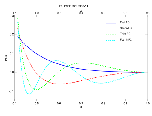
Figure 1: First four principal components built using the Union2.1 redshift coverage and a training set of $\Lambda$CDM models with the following sampling of the cosmological parameters: $0.1\leq\Omega_{\mathrm{m}}\leq 0.5$ and $0.5\leq\Omega_{\Lambda}\leq 0.9$.

In Fig. 1 we show the principal components obtained using the redshift coverage of Union2.1 and a training set of 11 flat $\Lambda$CDM models with the sampling $0.1\leq\Omega_{\mathrm{m}}\leq 0.5$ and $0.5\leq\Omega_{\Lambda}\leq 0.9$. The first principal component for this sample already accounts for $\approx 99.9\%$ of the total variance and its determination carries an uncertainty of $\sigma_{\mathrm{PC_{1}}}\approx 2.5\times 10^{-5}$. This means it already contains the main properties of the expansion of the Universe and accounts alone for a great part of the total variance sampled in the scatter matrix. Therefore, we restrict ourselves to only one principal component when performing the reconstruction.

Fitting the luminosity distance data to the expression in Eq. (6) with 1 PC returns $c_{1}=122.74\pm 796.68$ and $H_{0}=70.43\pm 0.33$. These specific values were obtained considering $D_{\mathrm{L}}|_{\rm ref}=\mathbf{\bar{t}}$. However we did test other reference models and, although the value for $c_{1}$ depends slightly on the choice of $D_{\mathrm{L}}|_{\rm ref}$, the final reconstruction and the minimised $H_{0}$ do not (this is not the case in general and is due to the fact that the space covered by the training set is in a volume tightly enclosing the data). It is worth mentioning that the errors we obtain for $H_{0}$ are purely statistical and only due to the minimization process. They are negligible compared with the calibration error. However, we present our best fit here to demonstrate that the reconstructed zero-point of $H(z)$ points towards a lower value than the standard approach. This trend has been confirmed by the Planck results (Planck Collaboration, et al., 2013).

The gray area in Fig. (2) represents the reconstructed expansion history within 3$\sigma$ errors. For the sake of comparison, the figure also shows the best-fit cosmology found by the original Union2.1 analysis, $\Omega_{\mathrm{m}}=0.277\pm 0.022$ (Suzuki et al., 2012) and the latest result reported by the Planck satellite team, $\Omega_{\mathrm{m}}=0.314\pm 0.020$ (Planck Collaboration, et al., 2013). In order to avoid confusion, only the best-fit curves are shown in Fig. (2). Both results are in marginal agreement with the behaviour we found for $H(a)$.

For the reasons exposed above, it is clear that our approach does not output fits to specific cosmological parameters. However, we can put our reconstruction in the context of $\Lambda$CDM models and find the range of $\Omega_{\mathrm{m}}$ values allowed by the behaviour we found for $H(a)$. Keeping fixed the value we found for $H_{0}$, we obtain $\Omega_{\mathrm{m}}=0.297\pm 0.020$ (red curve in Fig. 2). We emphasise that the magnitude of the error does not carry the same meaning as in the standard parametric analysis shown in Fig. 2. The determination of range of values for $\Omega_{\mathrm{m}}$ is merely a strategy to better compare our results. Unlike other analyses we are tracking only dynamical deviations from $\mathbf{\bar{t}}$, which causes the error bars to be small.

The results we found are significantly higher than the best-fit value obtained by the Union2.1 team ($\Omega_{\mathrm{m}}=0.277$ without systematics; blue curve in Fig. 2), and are in close agreement with the value reported by Planck. We show in Fig. (3) a more clear comparison of our results with others from the SNe Ia literature (all using SALT2 light curve fitter; Guy et al., 2007). We believe that the shift in our results towards the Planck values is an indication that SNe Ia cosmology should move beyond the parametrized approaches if it aims at dealing with small deviations from the standard values of the cosmological parameters present in the data. We want to stress again that we are not biased by any theoretical opinion towards a cosmological model, since we do not assume any specific form of the Friedmann equations. In fact, the method is a powerful tool to evaluate non-standard cosmologies as we tentatively showed in Benitez-Herrera et al. (2012) and plan to explore in a more rigorous way in future work.

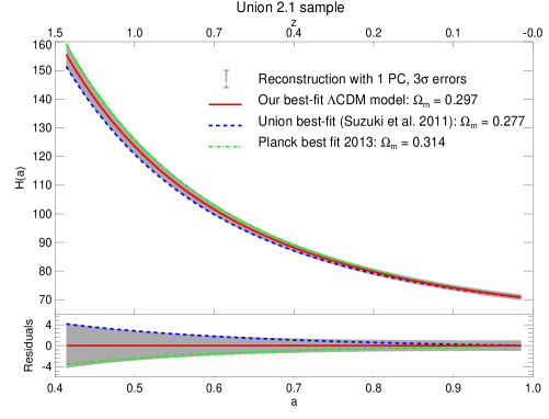
Figure 2: The reconstructed expansion history, with $3\sigma$ error, extracted from the Union2.1 sample using the optimal basis system with one PC. The red (solid) line represents our best-fit to $\Lambda$CDM paradigm. The blue (dashed) line is the best-fit obtained by the Union team for this sample and the green (dot-dashed) line corresponds to results from Planck.

Our model-independent method to constrain the expansion history has other interesting applications. For instance, it offers a complementary way of detecting possible systematic effects – e.g. the uncertainties introduced by the light curve calibration, host galaxy extinction or intrinsic variations corresponding to different SN Ia populations – which could affect the data and would be overlooked within a traditional analysis based on physical parameterizations. The method is also a valuable tool that can be used to plan future Type Ia supernova cosmology campaigns, by testing redshift ranges in which it would be more relevant to collect data (see Benitez-Herrera et al., 2012).

4 Conclusions

In this letter, we have applied a method to recover the expansion history of the Universe in a model-independent fashion. The luminosity-distance measurements, obtained from SNe Ia, depend only on space-time geometry, and can be directly related to the Hubble function without assuming any dynamical model. We argue that, as long as the nature of dark energy remains unknown, model-independent analyses of the kind described here have more significance in deriving cosmological parameters than traditional parametric studies. This is due to the fact that no specific form of the equation of state $w$ or the Hubble function is fixed in our approach. Our only assumption relies on the argument that the luminosity distance can be expanded into a series of orthonormal functions. This basis is chosen to be derived from PCA, in an attempt to control the number of coefficients to be included in our reconstruction in a rigorous way.

Our analysis shows that SNe data do point to a higher value of $\Omega_{\mathrm{m}}$, in contradiction with what was found with standard methods. Furthermore, this is in agreement with the last results driven by Planck and might be an indication that it is important to move beyond parametric fits.

The ultimate goal of this work is to discriminate among different cosmological models, such as $f(R)$ or DGP theories, based on very different physical assumptions, and, in this way, break the current degeneracy in the cosmological parameters. Further analysis on simulated data might point to caveats not appearing in real data analysis.

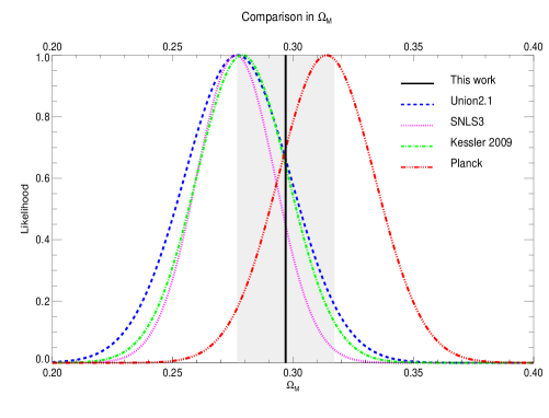
Figure 3: Comparison between our results when translated to flat $\Lambda$CDM scenario, $\Omega_{\mathrm{m}}=0.297\pm 0.020$ (gray region), and others from the literature. The green (dot-dashed) line correspond to results reported by the first year of SDSS data, $\Omega_{\mathrm{m}}=0.279\pm 0.019$ (Kessler et al., 2009). Cyan (dashed) line stands for results reported by Union2.1 team, $\Omega_{\mathrm{m}}=0.277\pm 0.022$ (Suzuki et al., 2012), the pink (dotted) line represents outcomes from SNLS3, $\Omega_{\mathrm{m}}=0.276\pm 0.016$ (Sullivan et al., 2011) and the red (dot-dot-dashed) line represents recent results from Planck, $\Omega_{\mathrm{m}}=0.314\pm 0.020$ (Planck Collaboration, et al., 2013). Only statistical errors are considered in this plot.

The model-independent method offers a complementary way of detecting possible systematic errors. This is especially relevant if one considers the dependence introduced by the light-curve fitters on the derived distances moduli from SNe Ia. It is important to test the performance of the available light-curve fitters on the base of model-independent approaches. A similar analysis of the same data set with different light curve fitters is important and will certainly be presented in a subsequent work.

Finally, is it worthwhile noting the potential of the method for the analysis of possible local inhomogeneities through comparison of the expansion history in different directions.

References

- Amanullah et al. (2010) Amanullah R., et al., 2010, ApJ, 716, 712
- Amendola et al. (2007) Amendola L., Gannouji R., Polarski D., Tsujikawa S., 2007, PhRvD, 75, 083504
- Arfken & Weber (1995) Arfken G. B., Weber H. J., 1995, Mathematical methods for physicists. Academic Press
- Astier et al. (2006) Astier P., et al., 2006, A&A, 447, 31
- Benitez-Herrera et al. (2012) Benitez-Herrera S., et al., 2012, MNRAS, 419, 513
- Daly & Djorgovski (2003) Daly R. A., Djorgovski S. G., 2003, ApJ, 597, 9
- Daly & Djorgovski (2004) Daly R. A., Djorgovski S. G., 2004, ApJ, 612, 652
- Eisenstein et al. (2005) Eisenstein D. J., et al., 2005, ApJ, 633, 560
- Fay & Tavakol (2006) Fay S., Tavakol R., 2006, PhRvD, 74, 083513
- Frieman et al. (1995) Frieman J. A., Hill C. T., Stebbins A., Waga I., 1995, Physical Review Letters, 75, 2077
- Guy et al. (2007) Guy J., et al., 2007, A&A, 466, 11
- Hamuy et al. (1996) Hamuy M., Phillips M. M., Suntzeff N. B., Schommer R. A., Maza J., Aviles R., 1996, AJ, 112, 2391
- Hicken et al. (2009) Hicken M., Wood-Vasey W. M., Blondin S., Challis P., Jha S., Kelly P. L., Rest A., Kirshner R. P., 2009, ApJ, 700, 1097
- Holtzman et al. (2008) Holtzman J. A., et al., 2008, AJ, 136, 2306
- Huterer & Peiris (2007) Huterer D., Peiris H. V., 2007, PhRvD, 75, 083503
- Huterer & Starkman (2003) Huterer D., Starkman G., 2003, Physical Review Letters, 90, 031301
- Ishida & de Souza (2011) Ishida E. E. O., de Souza R. S., 2011, A&A, 527, A49
- Ishida et al. (2011) Ishida E. E. O., de Souza R. S., Ferrara A., 2011, MNRAS, 418, 500
- Jollife (2002) Jollife I., 2002, A&A
- Kessler et al. (2009) Kessler R., et al., 2009, ApJS, 185, 32
- Kowalski et al. (2008) Kowalski M., et al., 2008, ApJ, 686, 749
- Maturi & Mignone (2009) Maturi M., Mignone C., 2009, A&A, 508, 45
- Mignone & Bartelmann (2008) Mignone C., Bartelmann M., 2008, A&A, 481, 295
- Miknaitis et al. (2007) Miknaitis G., et al., 2007, ApJ, 666, 674
- Perlmutter et al. (1999) Perlmutter S., et al., 1999, ApJ, 517, 565
- Planck Collaboration, et al. (2013) Planck Collaboration, Ade P. A. R., et al., 2013, ArXiv e-prints
- Riess et al. (1998) Riess A. G., et al., 1998, AJ, 116, 1009
- Riess et al. (2007) Riess A. G., et al., 2007, ApJ, 659, 98
- Seikel et al. (2012) Seikel M., Clarkson C., Smith M., 2012, JCAP, 6, 36
- Seikel & Schwarz (2008) Seikel M., Schwarz D. J., 2008, Journal of Cosmology and Astro-Particle Physics, 2, 7
- Seikel & Schwarz (2009) Seikel M., Schwarz D. J., 2009, Journal of Cosmology and Astro-Particle Physics, 2, 24
- Shafieloo (2007) Shafieloo A., 2007, MNRAS, 380, 1573
- Shafieloo et al. (2006) Shafieloo A., Alam U., Sahni V., Starobinsky A. A., 2006, MNRAS, 366, 1081
- Simpson & Bridle (2006) Simpson F., Bridle S., 2006, PhRvD, 73, 083001
- Spergel et al. (2003) Spergel D. N., et al., 2003, ApJS, 148, 175
- Starobinsky (1998) Starobinsky A. A., 1998, Soviet Journal of Experimental and Theoretical Physics Letters, 68, 757
- Sullivan et al. (2011) Sullivan M., et al., 2011, ApJ, 737, 102
- Suzuki et al. (2012) Suzuki N., et al., 2012, ApJ, 746, 85
- Turner & White (1997) Turner M. S., White M., 1997, PhRvD, 56, 4439