A comprehensive near and far ultraviolet spectroscopic study of the hot DA white dwarf G191-B2B

Abstract

We present a detailed spectroscopic analysis of the hot DA white dwarf G191-B2B, using the best signal to noise, high resolution near and far UV spectrum obtained to date. This is constructed from co-added HST STIS E140H, E230H, and FUSE observations, covering the spectral ranges of 1150-3145Å  and 910-1185Å  respectively. With the aid of recently published atomic data, we have been able to identify previously undetected absorption features down to equivalent widths of only a few mÅ. In total, 976 absorption features have been detected to $3\sigma$ confidence or greater, with 947 of these lines now possessing an identification, the majority of which are attributed to Fe and Ni transitions. In our survey, we have also potentially identified an additional source of circumstellar material originating from Si iii. While we confirm the presence of Ge detected by Vennes et al. (2005), we do not detect any other species. Furthermore, we have calculated updated abundances for C, N, O, Si, P, S, Fe, and Ni, while also calculating, for the first time, an NLTE abundance for Al, deriving Al iii/H=$1.60_{-0.08}^{+0.07}\times{10}^{-7}$. Our analysis constitutes what is the most complete spectroscopic survey of any white dwarf. All observed absorption features in the FUSE spectrum have now been identified, and relatively few remain elusive in the STIS spectrum.

1 Introduction

The archetype H rich white dwarf, G191-B2B (WD 0501+527), has long been used both as a photometric standard due to its apparent brightness, and also as a spectroscopic ”gold standard” when analysing other hot DA stars. This object has also been used as a flux standard at almost all wavelengths, beginning with the work of Oke (1974) to the absolute Hubble Space Telescope (HST) flux scale of Bohlin & Gilliland (2004). In Table 1, we list the basic stellar parameters of G191-B2B, where the mass, absolute magnitude ($M_{\nu}$) and cooling time ($t_{\mathrm{cool}}$) have been determined using the photometric tables of Holberg & Bergeron (2006); Kowalski & Saumon (2006); Tremblay et al. (2011); Bergeron et al. (2011) (hereafter the Montreal photometric tables).

The designation G191-B2B originates from the Giclas Lowell proper motion survey. While not formally identified as a white dwarf, Greenstein (1969) did identify it as being degenerate in nature, assigning it the spectral classification DAwk, and also designating it as a possible subdwarf. It was also listed by Eggen & Greenstein (1967) as a common proper motion pair with the K star G191-B2A, located 84” to the north. Such a proper motion pairing is now considered erroneous, as Hipparcos has shown the two stars to have distinctly different proper motions. G191-B2B is therefore an isolated star and efforts to determine a gravitational radial velocity from both stars (Reid & Wegner 1988 and Bergeron et al. 1995) are moot. A seminal high dispersion UV observation of G191-B2B by Bruhweiler & Kondo (1981), using the International Ultraviolet Explorer (IUE), revealed the surprising discovery of many highly ionised features such as C iv, N v, and Si iv in a star that was thought to possess a pure H spectrum. The detection of such absorption features led to extensive studies of other white dwarf stars. A decade later, the first detections of an ionised heavy metal, Fe v, were made by Sion et al. (1992) in the photospheric spectrum of G191-B2B using the HST Faint Object Spectrograph. This led to searches for additional heavy metals in white dwarf spectra, with the next Fe group metal, Ni, being discovered in G191-B2B and RE J2214-492 by Holberg et al. (1994), and Feige 24 and RE J0623-377 by Werner & Dreizler (1994), using co-added IUE high dispersion spectra. Further spectroscopic surveys were conducted, with yet more new heavy metals being discovered by Vennes et al. (1996), who made detections of the resonant transitions of P v and S vi in ORFEUS spectra. A later survey by Bruhweiler et al. (1999) used a spectrum from the HST, and discovered the presence of an additional component in the resonant lines of C iv 1548.203 and 1550.777Å  (hereafter C iv 1548 and 1550Å  respectively), that could not be attributed to either the photosphere of G191-B2B, or to the ISM. This feature was thought to be interstellar or “circumstellar” by Vennes & Lanz (2001), who in their survey of G191-B2B, showed that this feature was separated from the photospheric velocity by  15 km/s. This circumstellar material was not unique to G191-B2B, and similar high ionisation features were found in seven other DA white dwarfs by Bannister et al. (2003), corroborated by Dickinson et al. (2012b). The heaviest metal detected in a DA white dwarf thus far was found by Vennes et al. (2005), who made detections of resonant absorption features of Ge iv.

The Extreme Ultraviolet Explorer (EUVE), and the Joint Astrophysical Plasma-dynamic Experiment (J-PEX) (Bannister et al., 1999) have observed G191-B2B extensively, covering 70-770Å  and 170-290Å  respectively. EUVE observations of the star showed that the predicted flux far exceeded that observed (Kahn et al., 1984), meaning that model atmospheres for some effective temperature ($T_{\mathrm{eff}}$), gravity (log $g$), and composition could not simultaneously match the EUV, UV, and optical spectra. This was accomplished by Lanz et al. (1996), who showed that including additional opacity in model atmosphere calculations reduced the predicted flux to the correct level. However, this came at the cost of including additional He ii opacity in the photosphere in order to maintain good agreement below the He ii Lyman limit. An alternative was explored by Barstow et al. (1998), whereby they invoked a stratified H+He and homogeneous heavy metal atmosphere. While the model could also reproduce the EUV spectrum, it predicted He ii absorption features that descended far deeper than that observed. A substantial piece of work was done by Dreizler & Wolff (1999), who performed self consistent calculations including the effects of radiative levitation and gravitation settling for G191-B2B. By depleting the Fe and Ni abundance at the surface and having it increase at greater depths, they were able to reproduce the EUV spectrum without including other sources of opacity, mass loss, or accretion. A similar atmospheric configuration was used by Barstow et al. (1999), who stratified Fe, with increasing abundance with greater depth. They showed that this stratified configuration was preferred statistically over a homogeneous Fe distribution. Observations with J-PEX yielded further discoveries in the EUV spectrum of G191-B2B. Cruddace et al. (2002) performed a spectroscopic analysis of the star using J-PEX data, and made detections of the He ii Lyman series. This would be significant if it was found to be interstellar, as this would imply an unusual ionization fraction. It was also proposed that this He may be associated with the additional absorption component observed in the C iv doublet, discussed by Bruhweiler et al. (1999) and Vennes & Lanz (2001). A further spectroscopic survey using J-PEX was conducted by Barstow et al. (2005). They found that by splitting the He ii features into two components, one for the Local Interstellar Cloud, and the other as another interstellar feature, the He ionisation fraction agreed with values obtained from other lines of sight.

Observations of the H Lyman/Balmer line series of a white dwarf also allows information on its physical parameters to be inferred. Pioneered by Holberg et al. (1985), a grid of theoretical spectra with differing values of $T_{\mathrm{eff}}$ and log $g$ can be used to fit either the H Lyman or Balmer absorption profiles to that of an observed spectrum, as such profiles are very sensitive to changes in these parameters. Such a method, however, appears to have limitations for white dwarfs whose $T_{\mathrm{eff}}>$40,000K. Dubbed the ”Lyman-Balmer line problem”, measurements of $T_{\mathrm{eff}}$ made in DA white dwarfs using either the Lyman or Balmer line series yield differing values, some by a few 1,000K, and some even by 10,000K, getting larger for increasing values of $T_{\mathrm{eff}}$ (Barstow et al., 2003a). No similar appreciable effect is seen on the measurement of log $g$. A similar, more severe effect is seen in DAO stars (Good et al., 2004). A study by Lajoie & Bergeron (2007) considered many different causes of this problem, ranging from atmospheric composition to unresolved binaries. One such cause was concluded to be due to some form of wavelength dependent extinction, however, the exact relation between the two was left open to debate. It was also suggested that atmospheric composition may play a part in causing the discrepancy, but results were inconclusive. It is not unreasonable to consider such an idea, however, as metal line blanketing dramatically effects a hot DA SED. Barstow et al. (1998) have shown that using a model grid with a pure H atmosphere and a grid with a line blanketed heavy metal atmosphere yield $T_{\mathrm{eff}}$ measurements again differing by 1000s of K.

Barstow et al. (2003a) also considered the Lyman-Balmer line problem, postulating that the temperature discrepancy may be due to inadequacies in the input atomic physics in generating the model atmospheres. Using G191-B2B and RE J2214-492, they calculated two model grids with varying $T_{\mathrm{eff}}$ and log $g$, but with 0.1 and 10 times the nominal abundances of these stars. They then measured $T_{\mathrm{eff}}$ and log $g$ using the Lyman and Balmer line series, finding that while the temperature difference decreased by 20-30%, a statistically significant discrepancy still remained.

An accurate knowledge of a star’s photospheric composition is, therefore, paramount in accurately constraining $T_{\mathrm{eff}}$ and log $g$ in model atmosphere calculations. Determination of these parameters can provide useful insights into the white dwarf’s origin and evolution. For example, the cooling time of a degenerate object has a one to one correspondence with $T_{\mathrm{eff}}$, and hence gives a monotonic cooling age. Knowledge of log $g$ yields information on the mass of the white dwarf, and along with evolutionary models such as those from Wood (1998) or the Montreal Photometric Tables, an estimate of the radius of the star.

Calculations by Chayer et al. (1995a) for various values of $T_{\mathrm{eff}}$ and log $g$ describe the predicted variation of metal abundances due to radiative levitation. However, the observational results do not agree very well with the predictions. In the case of G191-B2B for example, Barstow et al. (2003b) reported the Fe and Ni abundances to be $3.30_{-1.20}^{+3.10}\times{10^{-6}}$ and $2.40_{-0.24}^{+0.84}\times{10^{-7}}$ respectively, differing roughly by an order of magnitude. However, Chayer et al. (1995a) predict that these abundances should share a similar value. This disagreement is also present in other white dwarfs in the sample of Barstow et al. (2003b). It should be noted, however, that Chayer et al. (1994) reported significant differences in predicted atmospheric abundances of Fe and Ni dependent on the number of transitions included in their calculations. It is this variation in results that suggests that poor agreement between theory and observation may be dependent on the number of opacities included in these calculations.

Table 1: A summary of the physical parameters of G191-B2B. The velocities $v_{\mathrm{LIC}}$ and $v_{\mathrm{Hyades}}$ are calculated along the line of sight to the star.

Parameter	Value	Reference
V	$11.727\pm{0.016}$	Holberg & Bergeron (2006)
$M_{v}$	$8.280\pm{0.164}$	This work
$T_{\mathrm{eff}}$ (K)	$52,500\pm{900}$	Barstow et al. (2003b)
Log $g$	$7.53\pm{0.09}$	Barstow et al. (2003b)
Mass ($M_{\odot}$)	$0.52\pm{0.035}$	This work
Radius ($R_{\odot}$)	$0.0204\pm{0.0014}$	This work
Distance (Pc)	$48.9\pm{3.7}$	This work
$t_{\mathrm{cool}}$ (Myr)	$1.50\pm{0.08}$	This work
$v_{\mathrm{phot}}$ (km s-1)	$23.8\pm{0.03}$	This work
$v_{\mathrm{LIC}}$ (km s-1)	$19.4\pm{0.03}$	This work
$v_{\mathrm{Hyades}}$ (km s-1)	$8.64\pm{0.03}$	This work

In this paper we present and analyse a unique spectrum of G191-B2B with unprecedented signal to noise (S/N), over the wavelength range 910-3145Å. The spectrum is constructed using co-added Far Ultraviolet Spectroscopic Explorer (FUSE) LWRS (30$\times$30”, low resolution), MDRS (4.0$\times$20”, medium resolution), and HIRS (1.21$\times$20”, high resolution) spectra, and co-added Space Telescope Imaging Spectrometer (STIS) E140H and E230H spectra. The resolution of our data sets range from 25,000 for the FUSE data to 144,000 for the HST spectra. The S/N exceeds 100 in many regions. We begin by describing the observational data used, and how co-addition of several data sets has allowed access to previously undetectable absorption lines. In section 3, we discuss the new atomic data releases provided by the Kurucz (Kurucz 1992, 2006, 2011, hereafter Kurucz) and Kentucky (hereafter Kentucky) databases and the effect this has had on our ability to identify new lines. A comprehensive table of identifications has been included in Appendix B. We calculate the atmospheric abundances of C, N, O, Al, Si, P, S, Fe, and Ni. We discuss a new potential circumstellar identification, and the abundance pattern of the white dwarf. The potential significance of including additional opacities into model atmosphere calculations is also discussed, providing a tentative solution to the Lyman-Balmer line problem. In summary, this data set is a unique and invaluable record of the archetype white dwarf G191-B2B. It is the most complete, and highest S/N NUV and FUV spectrum available for any white dwarf observed. It will serve as a template for studies of other hot white dwarfs, as a test bed for model atmosphere calculations, and also for the improvement of atomic databases.

2 Observational Data

Three detailed coadded spectra were used to analyse the NUV/FUV flux distribution of G191-B2B, spanning 910 to 3145Å. All data used in the coadded spectra are hosted on the Mikulski Archive for Space Telescopes (MAST). Using LWRS, MDRS, and HIRS exposures observed by FUSE, Barstow et al. (2010) constructed a coadded spectrum spanning 910-1185Å  with an exceptional S/N ratio. Observations by STIS aboard the HST covered the remainder of the spectrum. We made use of as many high resolution ($R\approx{144,000}$) observations with the echelle gratings E140H (centroid wavelength 1400Å) and E230H (centroid wavelength 2300Å) as possible, and produced a coadded spectrum spanning 1160-1680Å  and 1625-3145Å  respectively.

2.1 FUSE

FUSE was launched in 1999, providing coverage from 910Å  to 1185Å, making the Lyman series accessible to Ly $\beta$. While the satellite has been described many times (e.g. Moos 2000), we provide a brief summary of the hardware here. FUSE utilised a Rowland Circle design with four separate channels or coaligned optical paths. The satellite employed two detectors, each of which had two independent segments, SiC and LiF, upon which the spectra from the four channels are recorded. FUSE has three different aperture configurations, LWRS, MDRS and HIRS. FUSE also has a pinhole aperture (RFPT), which was mainly used for calibration. To minimise the possibility that the target’s light did not fall on the detector, observations were conducted primarily using the LWRS aperture, with a spectral resolution of 15,000-20,000 for early observations, and 23,000 for later ones, where the mirror focusing had been adjusted (Sahnow, 2000). Observations were also taken using both the TIMETAG (TTAG) and HISTOGRAM (HIST) modes. All FUSE data used here were reduced and processed using version 3.2 of calfuse (Dixon et al., 2007). The data comprises exposures from each of the detector/segment combinations (eight in total). We used the FUSE spectrum of G191-B2B from Barstow et al. (2010), constructed with 48 observations listed in Table 2, and plotted in Figure 1. The different observations were coadded according to the process described by Barstow et al. (2003a). Prior to coaddition, all spectra were rebinned to a common wavelength spacing to account for the difference in resolution between apertures. A consequence of coadding exposures from the different slits are discontinuities in the flux. It is for this reason we applied a correcting factor of 1.08 shortward of 1089Å  to ensure continuity between the FUSE and STIS flux distributions.

Table 2: The FUSE datasets obtained from MAST.

Observation ID	Number of exposures	Start time	Exposure time (s)	Aperture
M1010201000	8	13/10/99 01:25	4164	LWRS
M1030501000	1	12/11/99 07:35	266	MDRS
M1030502000	1	20/11/99 07:22	900	MDRS
M1030401000	1	20/11/99 09:02	1298	HIRS
M1030603000	5	20/11/99 10:43	3664	LWRS
M1030503000	3	21/11/99 06:43	1709	MDRS
M1030504000	4	21/11/99 10:03	3212	MDRS
M1030602000	5	21/11/99 11:39	2812	LWRS
S3070101000	32	14/01/00 09:40	15456	LWRS
M1010202000	7	17/02/00 06:10	3450	LWRS
M1030604000	1	09/01/01 09:02	503	LWRS
M1030506000	1	09/01/01 09:26	503	MDRS
M1030605000	1	10/01/01 13:20	503	LWRS
M1030507000	1	10/01/01 13:45	503	MDRS
M1030403000	2	10/01/01 15:08	483	HIRS
M1030606000	5	23/01/01 06:08	2190	LWRS
M1030508000	5	23/01/01 07:55	2418	MDRS
M1030404000	5	23/01/01 11:18	1853	HIRS
M1030607000	5	25/01/01 04:46	1926	LWRS
M1030509000	5	25/01/01 06:33	2417	MDRS
M1030405000	5	25/01/01 09:53	2419	HIRS
M1030608000	5	28/09/01 13:50	2728	LWRS
M1030510000	4	28/09/01 15:35	1910	MDRS
M1030406000	5	28/09/01 17:15	1932	HIRS
M1030609000	5	21/11/01 09:54	2703	LWRS
M1030511000	4	21/11/01 11:39	1910	MDRS
M1030407000	5	21/11/01 13:19	1932	HIRS
M1030610000	16	17/02/02 07:27	8639	LWRS
M1030512000	11	17/02/02 12:34	4757	MDRS
M1030408000	5	17/02/02 17:43	1932	HIRS
M1030611000	8	23/02/02 02:05	3645	LWRS
M1030513000	5	23/02/02 06:43	1797	MDRS
M1030409000	5	23/02/02 08:23	1921	HIRS
M1030612000	14	25/02/02 02:17	7004	LWRS
M1030514000	4	25/02/02 06:59	1617	MDRS
M1030613000	5	03/12/02 21:00	2358	LWRS
M1030614000	3	06/12/02 02:30	702	LWRS
M1030515000	4	06/12/02 05:16	2002	MDRS
M1052001000	16	07/12/02 21:46	7061	LWRS
M1030615000	4	08/12/02 22:36	1895	LWRS
M1030516000	4	09/12/02 00:29	1911	MDRS
M1030412000	4	09/12/02 03:53	1880	HIRS
M1030616000	4	05/02/03 19:14	1980	LWRS
M1030517000	4	05/02/03 21:07	1910	MDRS
M1030413000	4	06/02/03 00:36	1932	HIRS
M1030617000	8	23/11/03 20:16	4121	LWRS
M1030519000	4	25/01/04 21:31	1887	MDRS
M1030415000	4	26/01/04 00:51	1902	HIRS

Figure 1: Co-added spectrum of G191-B2B using 48 FUSE observations from LWRS, MDRS, and HIRS apertures.

2.2 STIS

G191-B2B has been extensively observed as a calibration standard by HST. In particular, observations of this star were conducted as part of Cycle 8 STIS calibration programs 8067, 8421 and 8915, which were designed to provide flux calibrations at the 1% level for all E140H and E230H primary and secondary echelle grating modes with a strong stellar continuum source. After the 2009 repair mission STS-125, an additional calibration program 11866 was proposed in Cycle 17 in order to evaluate the post-repair echelle blaze dependence on MSM position. The data were obtained in the ACCUM mode in four periods; 17th December 1998, 16th to 19th March 2000, 17th to 19th September 2001, and 28th November 2009 to 6th January 2010. Standard target acquisition procedures were used to acquire the source and centre it within the 0.2$\times$0.2” slit. The wavelength range 1140-3145Å  was covered by using all nine STIS primary grating settings and 28 secondary grating settings (see Chapter 11 of Hernandez 2012).

We examined all of the available E140H and E230H datasets (39 and 77 respectively) from the MAST website in order to check for discontinuities and errors in the observations. We found that 32 E140H and 66 E230H observations were free of such problems, and were hence included in the final coadded product, with total exposure times of 53318 and 77743s respectively. We summarise the individual STIS spectra in Table 4. After the extraction of the echelle orders, including ripple correction, the spectra were interpolated on to a single linear wavelength scale prior to exposure time weighted coaddition. The result was two single continuous spectra as shown in Figure 2. The distribution of S/N as a function of wavelength is shown in Figure 3.

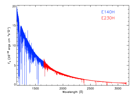
Figure 2: The final coadded spectra for the E140H (blue in online copy) and the E230H spectra (red in online copy). Most of the features falling below the continuum are identified absorption features.

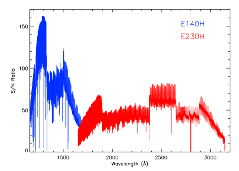
Figure 3: The dependence of signal to noise with wavelength. The wavelength ranges (and colour scheme in the online version) are the same as for Figure 2.

Table 3: A list of exposures used in the STIS spectrum coaddition. Where $\lambda_{c}$ is the central wavelength of the exposure, P is the primary setting, and S is the secondary setting.

Observation ID	Date	Prog. ID	Grating	$\lambda_{c}$ (Å)	Setting	Exposure time (s)
O57U01020	17/12/1998 08:17	8067	E140H	1416	P	2040
O57U01030	17/12/1998 09:34	8067	E140H	1234	P	2789
O57U01040	17/12/1998 11:14	8067	E140H	1598	P	2703
O5I010010	16/03/2000 23:31	8421	E140H	1234	P	2279
O5I010020	17/03/2000 00:52	8421	E140H	1234	P	3000
O5I010030	17/03/2000 02:29	8421	E140H	1234	P	3000
O5I011010	17/03/2000 04:21	8421	E140H	1598	P	2284
O5I011020	17/03/2000 05:42	8421	E140H	1598	P	3000
O5I011030	17/03/2000 07:18	8421	E140H	1598	P	3000
O5I014010	18/03/2000 02:52	8421	E230H	2513	P	2304
O5I014020	18/03/2000 04:14	8421	E230H	2513	P	3000
O5I014030	18/03/2000 05:50	8421	E230H	2513	P	3000
O5I015010	18/03/2000 22:10	8421	E230H	3012	P	2304
O5I015020	18/03/2000 23:32	8421	E230H	3012	P	3000
O5I015030	19/03/2000 01:09	8421	E230H	3012	P	3000
O5I013010	19/03/2000 03:00	8421	E230H	1763	P	2304
O5I013020	19/03/2000 04:22	8421	E230H	1763	P	3000
O5I013030	19/03/2000 05:59	8421	E230H	1763	P	3000
O6HB40080	12/09/2001 23:09	8915	E230H	2413	S	774
O6HB40090	13/09/2001 00:08	8915	E230H	3012	P	2228
O6HB10010	17/09/2001 13:49	8915	E140H	1234	P	867
O6HB10020	17/09/2001 14:05	8915	E140H	1234	P	867
O6HB10040	17/09/2001 14:54	8915	E140H	1271	S	640
O6HB10050	17/09/2001 15:11	8915	E140H	1307	S	654
O6HB10080	17/09/2001 16:30	8915	E140H	1380	S	719
O6HB10090	17/09/2001 16:48	8915	E140H	1416	P	851
O6HB100A0	17/09/2001 17:09	8915	E140H	1453	S	809
O6HB100B0	17/09/2001 18:07	8915	E140H	1453	S	229
O6HB100C0	17/09/2001 18:17	8915	E140H	1489	S	1263
O6HB100D0	17/09/2001 18:44	8915	E140H	1526	S	887
O6HB100E0	17/09/2001 19:43	8915	E140H	1526	S	749
O6HB100F0	17/09/2001 20:02	8915	E140H	1562	S	1996
O6HB20010	18/09/2001 15:32	8915	E230H	1763	P	1314
O6HB20020	18/09/2001 16:00	8915	E230H	1813	S	654
O6HB20030	18/09/2001 16:35	8915	E230H	1813	S	455
O6HB20040	18/09/2001 16:49	8915	E230H	1863	S	997
O6HB20050	18/09/2001 17:12	8915	E230H	1913	S	907
O6HB20060	18/09/2001 18:11	8915	E230H	1963	S	871
O6HB20070	18/09/2001 18:32	8915	E230H	2013	P	808
O6HB20080	18/09/2001 18:51	8915	E230H	2063	S	718
O6HB20090	18/09/2001 19:47	8915	E230H	2113	S	679
O6HB200A0	18/09/2001 20:05	8915	E230H	2163	S	640
O6HB200B0	18/09/2001 20:21	8915	E230H	2213	S	620
O6HB200C0	18/09/2001 20:38	8915	E230H	2263	P	101
O6HB200D0	18/09/2001 21:24	8915	E230H	2263	P	609.6
O6HB200E0	18/09/2001 21:40	8915	E230H	2313	S	734.3
O6HB200F0	18/09/2001 21:59	8915	E230H	2363	S	748.7
O6HB30010	19/09/2001 15:39	8915	E230H	2463	S	668
O6HB30020	19/09/2001 15:56	8915	E230H	2513	P	696
O6HB30030	19/09/2001 16:13	8915	E230H	2563	S	247
O6HB30040	19/09/2001 16:39	8915	E230H	2563	S	484
O6HB30050	19/09/2001 16:54	8915	E230H	2613	S	769
O6HB30060	19/09/2001 17:13	8915	E230H	2663	S	992.3
O6HB30070	19/09/2001 18:16	8915	E230H	2713	S	900
O6HB30080	19/09/2001 18:37	8915	E230H	2762	P	978
O6HB30090	19/09/2001 18:59	8915	E230H	2812	S	519
O6HB300A0	19/09/2001 19:52	8915	E230H	2812	S	578
O6HB300B0	19/09/2001 20:08	8915	E230H	2862	S	1232
O6HB300C0	19/09/2001 20:35	8915	E230H	2912	S	549
O6HB300D0	19/09/2001 21:28	8915	E230H	2912	S	873

Table 4: continued

Observation ID	Date	Prog. ID	Grating	$\lambda_{c}$ (Å)	Setting	Exposure time (s)
O6HB300E0	19/09/2001 21:49	8915	E230H	2962	S	1862
OBB002010	28/11/2009 08:36	11866	E230H	1863	S	1000
OBB002020	28/11/2009 08:59	11866	E230H	1963	S	870
OBB002030	28/11/2009 09:55	11866	E230H	1913	S	920
OBB002040	28/11/2009 10:16	11866	E230H	2013	P	810
OBB002050	28/11/2009 10:36	11866	E230H	2063	S	740
OBB002060	28/11/2009 11:31	11866	E230H	2263	P	800
OBB002070	28/11/2009 11:50	11866	E230H	2113	S	850
OBB002080	28/11/2009 12:10	11866	E230H	2163	S	800
OBB002090	28/11/2009 13:07	11866	E230H	1763	P	1800
OBB0020A0	28/11/2009 13:43	11866	E230H	2213	S	1000
OBB0020B0	28/11/2009 14:43	11866	E230H	1813	S	1160
OBB0020C0	28/11/2009 15:08	11866	E230H	2313	S	650
OBB0020D0	28/11/2009 15:25	11866	E230H	2363	S	650
OBB004080	29/11/2009 12:12	11866	E230H	2413	S	645
OBB004090	29/11/2009 13:05	11866	E230H	3012	P	2192
OBB001010	30/11/2009 06:58	11866	E140H	1271	S	696
OBB001020	30/11/2009 07:15	11866	E140H	1453	S	1038
OBB001030	30/11/2009 08:16	11866	E140H	1380	S	752
OBB001040	30/11/2009 08:34	11866	E140H	1234	P	867
OBB001050	30/11/2009 08:54	11866	E140H	1416	P	851
OBB001070	30/11/2009 10:09	11866	E140H	1526	S	2100
OBB001080	30/11/2009 11:27	11866	E140H	1562	S	2134
OBB001090	30/11/2009 12:09	11866	E140H	1307	S	654
OBB0010A0	30/11/2009 13:03	11866	E140H	1489	S	1200
OBB005010	01/12/2009 05:12	11866	E140H	1234	P	2200
OBB005020	01/12/2009 06:38	11866	E140H	1234	P	6200
OBB053010	06/01/2010 13:30	11866	E230H	2563	S	900
OBB053020	06/01/2010 13:51	11866	E230H	2613	S	950
OBB053030	06/01/2010 14:43	11866	E230H	2663	S	830
OBB053040	06/01/2010 15:03	11866	E230H	2463	S	670
OBB053050	06/01/2010 15:20	11866	E230H	2713	S	900
OBB053060	06/01/2010 16:19	11866	E230H	2762	P	1197
OBB053070	06/01/2010 16:45	11866	E230H	2862	S	1647
OBB053080	06/01/2010 17:55	11866	E230H	2513	P	1000
OBB053090	06/01/2010 18:18	11866	E230H	2912	S	1800
OBB0530A0	06/01/2010 19:31	11866	E230H	2812	S	1097
OBB0530B0	06/01/2010 19:55	11866	E230H	2962	S	1747

3 Line survey

3.1 Atomic data

We combined data from the Kurucz and Kentucky atomic databases to compile as complete a line list as possible. The Kurucz database has been updated several times, with major updates occurring in 1992, 2006, and 2011 (Kurucz, 1992, 2006, 2011). Table 5 shows how the number of transitions available for Fe iv-vii and Ni iv-vii have increased from the 1992 to the 2011 data releases; an order of magnitude increase in the number of transitions is seen for each ion. Figure 4 illustrates the improvement made in reproducing the 980-1020Å  spectral region of G191-B2B using the 1992 Kurucz data release and some lines from the National Institute of Standards and Technology (NIST), and our combined line list, synthesised using the model atmosphere of Barstow et al. (2003b). Some transitions in the Kentucky database lacked oscillator strengths ($f$-values). For Figure 4, we set the missing $f$-values to $1.00\times{10}^{-6}$ for illustrative purposes. We choose this value as weak Fe/Ni transitions have oscillator strengths $\sim{10^{-6}}$. The Kurucz and Kentucky databases often had records of the same transition. For the purposes of identification, we used the data from the Kentucky database, as this supplies errors on the laboratory wavelengths of transitions. To identify resonant transitions, we used the line list of Verner et al. (1994) (hereafter V94), and found the error on the wavelength by cross-correlating this line list with the Kentucky database.

Table 5: The number of lines present in the Kurucz linelist in 1992 and 2011 for Fe and Ni iv-vii.

Ion	No of lines 1992	No of lines 2011
Fe iv	1,776,984	14,617,228
Fe v	1,008,385	7,785,320
Fe vi	475,750	9,072,714
Fe vii	90,250	2,916,992
Ni iv	1,918,070	15,152,636
Ni v	1,971,819	15,622,452
Ni vi	2,211,919	17,971,672
Ni vii	967,466	28,328,012
Total	10,420,643	111,467,026

Figure 4: A comparison of the predicted synthetic (upper line) spectrum to the observed spectrum (bottom line). In the top plot, the spectrum has been synthesised using only the 1992 Kurucz data release and some lines from NIST (described in text), whereas in the bottom plot, the spectrum has been synthesised using both the 2011 Kurucz and Kentucky data releases. The synthetic spectrum has been offset for clarity.

3.2 Absorption feature parameterisation

For the purposes of identification, we need to extract the basic parameters of each absorption feature, such as wavelength centroid, velocity, and equivalent width. To parameterise the absorption feature as accurately as possible, we fit a Gaussian and Lorentzian profile (see Appendix A for the exact parameterisation) to the feature with a chi squared ($\chi^{2}$) minimisation technique, using the IDL routine mpfit (Markwardt, 2009). The fit that achieved the lowest $\chi^{2}$ was assumed to be the best fit. Hence we used the calculated parameters from this fit. To differentiate between signal and noise, we adopted a $3\sigma$ threshold. In the cases where absorption features appeared to be blended, we used a double Gaussian absorption profile (see also Appendix A).

3.3 Detections and identification

We detected 976 absorption features, successfully identifying 947 of them. Lines that could not be identified are listed in Table 6. Several measured lines in our survey were found to be the result of multiple blended features. Therefore, the velocity of each individual absorber was included in calculating the weighted velocity of each component. To calculate the uncertainty on the velocity measurements, the uncertainties in the measured wavelength ($\lambda_{\mathrm{tot}}$) were obtained by adding in quadrature the uncertainties in laboratory ($\delta\lambda_{\mathrm{lab}}$) and observed wavelength ($\delta\lambda_{\mathrm{obs}}$) calculated from the Gaussian/Lorentzian fit. Some velocity uncertainties were anomalously high due to large uncertainties from the Kentucky database, and it is for this reason that the average photospheric and interstellar velocities were calculated by weighting each line velocity by its inverse error:

$$\bar{v}=\frac{\sum_{i=1}^{N}\frac{v_{i}}{\delta{v_{i}}^{2}}}{\sum_{i=1}^{N}\frac{1}{\delta{v_{i}}^{2}}}$$ (1)

With associated error:

$$\delta\bar{v}=\sqrt{\frac{1}{\sum_{i=1}^{N}\frac{1}{\delta{v_{i}}^{2}}}}$$ (2)

Where $v_{i}$ and $\delta{v_{i}}$ are the line velocities and their respective errors, and $N$ is the number of lines used to calculate the mean. The velocities were calculated using only lines with wavelength errors from Kentucky, and were observed in the STIS data. In our line survey, we identified three definitive velocity populations, one photospheric, and two interstellar. We measured the photospheric velocity as $23.8\pm{0.03}$km s^-1, while the interstellar velocities were measured as $19.4\pm{0.03}$km s^-1 and $8.64\pm{0.03}$km s^-1 respectively. In Table 7, we compare our photospheric velocity with that obtained by Vennes & Lanz (2001), and our interstellar velocities with those from Redfield & Linsky (2008). Hereafter, we refer to the interstellar velocities by the name of the cloud from which they appear to originate, as named by Redfield & Linsky (2008), where the $19.4\pm{0.03}$km s^-1 velocity corresponds to the Local Interstellar Cloud (LIC), and the $8.64\pm{0.03}$km s^-1 velocity to the Hyades Cloud. The velocities determined in this study appear to be in excellent agreement with those obtained by previous authors.

Table 6: A list of absorption features that could not be identified in our survey, where $\lambda_{\mathrm{Obs}}$ is the observed wavelength with accompanying error $\delta\lambda_{\mathrm{Obs}}$, and $W_{\lambda}$ is the equivalent width, with error $\delta{W_{\lambda}}$.

$\lambda_{\mathrm{Obs}}$(Å)	$\delta\lambda_{\mathrm{Obs}}$(mÅ)	$W_{\lambda}$(mÅ)	$\delta{W_{\lambda}}$(mÅ)
1171.277	1.9730	2.584	0.793
1174.424	1.3261	5.417	0.843
1186.174	2.8080	3.046	0.962
1186.355	0.9279	9.953	0.927
1196.733	1.7920	3.897	0.730
1198.240	0.9257	6.856	0.636
1199.443	1.0994	2.369	0.572
1201.548	2.2597	1.689	0.543
1204.561	2.0988	3.064	0.613
1206.756	1.4513	3.354	0.686
1206.812	2.4298	2.788	0.761
1228.604	2.9613	3.232	0.663
1232.311	3.4623	1.813	0.554
1253.405	2.0101	1.727	0.472
1255.177	3.0864	2.695	0.329
1270.950	4.4021	4.710	0.558
1274.017	1.8103	1.920	0.386
1285.088	2.8810	1.148	0.359
1291.912	2.3123	3.007	0.586
1292.590	2.7298	2.880	0.578
1295.987	2.6044	1.651	0.311
1302.927	2.8485	3.624	0.653
1318.082	1.0165	2.999	0.353
1321.307	1.4181	2.564	0.403
1322.416	1.3813	2.398	0.375
1333.462	2.3978	2.265	0.613
1442.574	2.4808	1.673	0.401
1499.254	3.6779	3.035	0.827
1513.608	3.2663	2.266	0.730

Table 7: A summary of the velocity populations identified in the spectrum. Each velocity was calculated using the weighted mean of the various line velocities measured in the STIS data. We also compare our determined photospheric velocity to that determined by Vennes & Lanz (2001), and our ISM velocities with that of Redfield & Linsky (2008).

Origin	$v_{\mathrm{Current}}$ (km s-1)	$v_{\mathrm{Previous}}$ (km s-1)
Photosphere	$23.8\pm{0.03}$	$24.3\pm{1.7}$
LIC	$19.4\pm{0.03}$	$19.19\pm{0.09}$
Hyades	$8.64\pm{0.03}$	$8.61\pm{0.74}$

4 Model atmospheres and abundance determination

To determine the abundances, we first used tlusty version 200 to calculate a model atmosphere based on the abundances given by Barstow et al. (2003b) (C, N, O, Si, Fe, Ni) and Vennes & Lanz (2001) (P, S) in NLTE. We fixed He/H to $1.00\times{10^{-5}}$, and $T_{\mathrm{eff}}$ and log $g$ to 52,500K and 7.53 respectively. The model atoms used by tlusty, along with the number of levels included, are listed in Table 8. Next, as Al had not been included in a full NLTE model atmosphere calculation for G191-B2B before, we introduced the metal into the solution, and calculated a grid of models with varying Al abundances, the values of which are given in Table 9. The model spectra were then synthesized using synspec version 49, and Kurucz’s 1992 line list as this has a complete set of oscillator strengths. It was interesting to note that even with the greatest abundance of Al, there was no noticable flux redistribution. We then determined the Al abundance using xspec (Arnaud, 1996), which we will describe shortly. Upon determining the abundance, we recalculated the atmosphere with this value using tlusty. As the abundances of C, N, O, Si, P, S, Fe and Ni are not so different from the values derived in Barstow et al. (2003b) and Vennes & Lanz (2001), any flux redistribution due to small abundance variations is likely to be a second order effect. Therefore, instead of calculating a model atmosphere for each metal, which is computationally expensive, we used synspec 49 to modify the abundances, creating a model grid for each metal as given in Table 9, again using the 1992 Kurucz line list. As with Al, we then used xspec to determine the abundances.

xspec calculates the abundances and associated errors by taking a model atmosphere grid and observational data as input, and interpolating between the different abundance values using a chi square ($\chi^{2}$) minimisation technique. xspec has difficulty in performing computations with spectra containing many data points. With 60,000 data points, the STIS spectrum can not, therefore, be analysed in its entirety without dividing it into segments. Therefore, we extracted small regions of spectra containing the absorption features that we wish to analyse, summarised in Table 10. Isolating small sections of spectrum also has the advantage of minimising systematic errors due to poor normalisation of the continuum whilst fitting the abundances. We determined the abundance of each metal ionisation stage individually. In cases where there were multiple lines in an ionisation stage, we fixed the abundance to be the same for each feature. Photospheric features that appeared to be blended with additional components were modelled by including an additional Gaussian absorber using the xspec model gabs (see Appendix A for the exact parameterisation) as done by Dickinson et al. (2012c). In all cases, we quote our formal errors to $1\sigma$ confidence, and assume one degree of freedom except where noted. We have tabulated our abundance determinations in Table 11. We have also tabulated the parameter values and their respective errors obtained from fitting the gabs component in Table 12, along with the velocity of the absorber where relevant.

Table 8: Model atoms used in calculating the initial model atmosphere.

Element	Ion	No of Levels
H	i	9
He	i	24
He	ii	20
C	iii	23
C	iv	41
N	iii	32
N	iv	23
N	v	16
O	iv	39
O	v	40
O	vi	20
Si	iii	30
Si	iv	23
P	iv	14
P	v	17
S	iv	15
S	v	12
S	vi	16
Fe	iv	43
Fe	v	42
Fe	vi	32
Ni	iv	38
Ni	v	48
Ni	vi	42

Table 9: The grid of abundances used in fitting the metal absorption features. $T_{\mathrm{eff}}$ and log $g$ were fixed at 52500K and 7.53 respectively.

C	N	O	Al	Si	P	S	Fe	Ni
$2.00\times{10}^{-8}$	$2.00\times{10}^{-8}$	$2.00\times{10}^{-8}$	$2.00\times{10}^{-8}$	$2.00\times{10}^{-8}$	$2.00\times{10}^{-9}$	$2.00\times{10}^{-8}$	$2.00\times{10}^{-7}$	$2.00\times{10}^{-8}$
$6.00\times{10}^{-8}$	$6.00\times{10}^{-8}$	$6.00\times{10}^{-8}$	$6.00\times{10}^{-8}$	$6.00\times{10}^{-8}$	$6.00\times{10}^{-9}$	$6.00\times{10}^{-8}$	$6.00\times{10}^{-7}$	$6.00\times{10}^{-8}$
$2.00\times{10}^{-7}$	$2.00\times{10}^{-7}$	$2.00\times{10}^{-7}$	$2.00\times{10}^{-7}$	$2.00\times{10}^{-7}$	$2.00\times{10}^{-8}$	$2.00\times{10}^{-7}$	$2.00\times{10}^{-6}$	$2.00\times{10}^{-7}$
$6.00\times{10}^{-7}$	$6.00\times{10}^{-7}$	$6.00\times{10}^{-7}$	$6.00\times{10}^{-7}$	$6.00\times{10}^{-7}$	$6.00\times{10}^{-8}$	$6.00\times{10}^{-7}$	$6.00\times{10}^{-6}$	$6.00\times{10}^{-7}$
$2.00\times{10}^{-6}$	$2.00\times{10}^{-6}$	$2.00\times{10}^{-6}$	$2.00\times{10}^{-6}$	$2.00\times{10}^{-6}$	$2.00\times{10}^{-7}$	$2.00\times{10}^{-6}$	$2.00\times{10}^{-5}$	$2.00\times{10}^{-6}$

Table 10: The list of lines examined to determine the abundances of the photospheric metals, and the spectral window extracted to perform the analysis.

Ion	Wavelength (Å)	$f$-value	Spectral Region (Å)	Ion	Wavelength (Å)	$f$-value	Spectral Region (Å)
C iii	1174.9327	0.114	1174-1178	Fe iv	1592.050	0.3341	1590-1605
C iii	1175.263	0.274	1174-1178	Fe iv	1601.652	0.3379	1590-1605
C iii	1175.5903	0.069	1174-1178	Fe iv	1603.177	0.2679	1590-1605
C iii	1175.7112	0.205	1174-1178	Fe v	1280.470	0.0236	1280-1290
C iii	1175.9871	0.091	1174-1178	Fe v	1287.046	0.0363	1280-1290
C iii	1176.3697	0.068	1174-1178	Fe v	1288.172	0.0541	1280-1290
C iii	1247.383	0.163	1245-1255	Fe v	1293.382	0.0330	1290-1300
C iv	1548.202	0.190	1545-1555	Fe v	1297.549	0.0440	1290-1300
C iv	1550.777	0.095	1545-1555	Fe v	1311.828	0.1710	1305-1315
N iv	1718.551	0.173	1715-1725	Fe v	1320.409	0.1944	1320-1333
N v	1238.821	0.156	1235-1245	Fe v	1321.489	0.0905	1320-1333
N v	1242.804	0.078	1235-1245	Fe v	1323.271	0.1930	1320-1333
O iv	1338.615	0.118	1334-1344	Fe v	1330.405	0.2085	1320-1333
O iv	1342.99	0.011	1334-1344	Fe v	1331.189	0.0774	1320-1333
O iv	1343.514	0.104	1334-1344	Fe v	1331.639	0.1867	1320-1333
Al iii	1854.716	0.556	1850-1860	Ni iv	1356.079	0.0963	1350-1360
Al iii	1862.79	0.277	1860-1870	Ni iv	1398.193	0.3837	1395-1405
Si iii	1206.4995	1.610	1200-1210	Ni iv	1399.947	0.2964	1395-1405
Si iii	1206.5551	1.640	1200-1210	Ni iv	1400.682	0.2950	1395-1405
Si iv	1122.4849	0.819	1120-1130	Ni iv	1411.451	0.3507	1410-1422
Si iv	1128.3248	0.0817	1120-1130	Ni iv	1416.531	0.1949	1410-1422
Si iv	1128.3400	0.736	1120-1130	Ni iv	1419.577	0.1309	1410-1422
Si iv	1393.7546	0.508	1390-1400	Ni iv	1421.216	0.2863	1410-1422
Si iv	1402.7697	0.252	1400-1410	Ni iv	1430.190	0.1794	1425-1435
P iv	950.657	1.470	945-955	Ni iv	1432.449	0.1253	1425-1435
P v	1117.977	0.467	1115-1125	Ni iv	1452.220	0.3596	1450-1460
P v	1128.008	0.231	1125-1135	Ni iv	1498.893	0.1618	1495-1505
S iv	1062.662	0.052	1060-1070	Ni v	1230.435	0.2649	1230-1240
S iv	1072.974	0.045	1070-1080	Ni v	1232.807	0.1764	1230-1240
S vi	933.378	0.433	930-940	Ni v	1233.257	0.1605	1230-1240
S vi	944.523	0.213	940-950	Ni v	1234.393	0.1334	1230-1240
Fe iv	1542.155	0.1386	1540-1550	Ni v	1235.831	0.1982	1230-1240
Fe iv	1542.697	0.2818	1540-1550	Ni v	1236.277	0.1094	1230-1240
Fe iv	1544.486	0.2511	1540-1550	Ni v	1239.552	0.1116	1230-1240
Fe iv	1546.404	0.2070	1540-1550	Ni v	1241.627	0.2003	1240-1250
Fe iv	1562.751	0.2032	1560-1572	Ni v	1243.504	0.0815	1240-1250
Fe iv	1568.276	0.3012	1560-1572	Ni v	1243.662	0.1194	1240-1250
Fe iv	1569.222	0.1291	1560-1572	Ni v	1244.027	0.0503	1240-1250
Fe iv	1570.178	0.3147	1560-1572	Ni v	1245.176	0.2348	1240-1250
Fe iv	1570.416	0.2741	1560-1572

Table 11: Summary of the abundances determined in this work, along with $1\sigma$ errors.

Ion	Abundance	$-1\sigma$	$+1\sigma$
C iii	$1.72\times{10}^{-7}$	$0.02\times{10}^{-7}$	$0.02\times{10}^{-7}$
C iv	$2.13\times{10}^{-7}$	$0.15\times{10}^{-7}$	$0.29\times{10}^{-7}$
N iv	$1.58\times{10}^{-7}$	$0.14\times{10}^{-7}$	$0.14\times{10}^{-7}$
N v	$2.16\times{10}^{-7}$	$0.04\times{10}^{-7}$	$0.09\times{10}^{-7}$
O iv	$4.12\times{10}^{-7}$	$0.08\times{10}^{-7}$	$0.08\times{10}^{-7}$
Al iii	$1.60\times{10}^{-7}$	$0.08\times{10}^{-7}$	$0.07\times{10}^{-7}$
Si iii	$3.16\times{10}^{-7}$	$0.30\times{10}^{-7}$	$0.31\times{10}^{-7}$
Si iv	$3.68\times{10}^{-7}$	$0.14\times{10}^{-7}$	$0.13\times{10}^{-7}$
P iv	$8.40\times{10}^{-8}$	$1.18\times{10}^{-8}$	$1.18\times{10}^{-8}$
P v	$1.64\times{10}^{-8}$	$0.02\times{10}^{-8}$	$0.02\times{10}^{-8}$
S iv	$1.71\times{10}^{-7}$	$0.02\times{10}^{-7}$	$0.02\times{10}^{-7}$
S vi	$5.23\times{10}^{-8}$	$0.13\times{10}^{-8}$	$0.10\times{10}^{-8}$
Fe iv	$1.83\times{10}^{-6}$	$0.03\times{10}^{-6}$	$0.03\times{10}^{-6}$
Fe v	$5.00\times{10}^{-6}$	$0.06\times{10}^{-6}$	$0.06\times{10}^{-6}$
Ni iv	$3.24\times{10}^{-7}$	$0.05\times{10}^{-7}$	$0.13\times{10}^{-7}$
Ni v	$1.01\times{10}^{-6}$	$0.03\times{10}^{-6}$	$0.03\times{10}^{-6}$

Table 12: The best fitting xspec Gaussian model parameters for a given transition, where $\lambda_{\mathrm{lab}}$ is the lab wavelength, $E_{l}$ is the centroid wavelength of the Gaussian in keV, $\sigma_{l}$ is the line width of the Gaussian in keV, $\tau_{l}$ is the strength, and $v$ is the corresponding velocity of the absorber. All parameters have been calculated to $1\sigma$ confidence.

Ion	Parameter	Value	$-1\sigma$	$+1\sigma$
C iv	$\lambda_{\mathrm{lab}}$ (Å)	1548.203	-	-
	$E_{l}$ ($10^{-3}$keV)	8.008122	0.0000047	0.0000038
	$\sigma_{l}$ ($10^{-7}$keV)	1.34141	0.03611	0.03689
	Strength ($10^{-7}$)	1.19420	0.0426	0.0489
	$\lambda_{\mathrm{obs}}$ (Å)	1548.246	0.000735	0.000909
	$v$ (km s-1)	8.26	0.14	0.18
C iv	$\lambda_{\mathrm{lab}}$ (Å)	1550.777	-	-
	$E_{l}$ ($10^{-3}$keV)	7.994829	0.0000036	0.0000040
	$\sigma_{l}$ ($10^{-7}$keV)	1.26307	0.03597	0.02623
	Strength ($10^{-7}$)	7.18607	0.20447	0.17263
	$\lambda_{\mathrm{obs}}$ (Å)	1550.820	0.000776	0.000698
	$v$ (km s-1)	8.30	0.15	0.13
Si iii	$\lambda_{\mathrm{lab}}$ (Å)	1206.4995	-	-
	$E_{l}$ ($10^{-3}$keV)	10.276140	0.0000070	0.0000020
	$\sigma_{l}$ ($10^{-7}$keV)	0.925806	0.026966	0.025814
	Strength ($10^{-7}$)	4.79551	0.13501	0.14099
	$\lambda_{\mathrm{obs}}$ (Å)	1206.537	0.000235	0.000822
	$v$ (km s-1)	9.24	0.06	0.20
Si iv	$\lambda_{\mathrm{lab}}$ (Å)	1393.7546	-	-
	$E_{l}$ ($10^{-3}$keV)	8.895525	0.0000277	0.0000208
	$\sigma_{l}$ ($10^{-7}$keV)	0.926033	0.183263	0.293867
	Strength ($10^{-7}$)	0.434293	0.072113	0.098237
	$\lambda_{\mathrm{obs}}$ (Å)	1393.795	0.003259	0.004340
	$v$ (km s-1)	8.73	0.70	0.93
Si iv	$\lambda_{\mathrm{lab}}$ (Å)	1402.7697	-	-
	$E_{l}$ ($10^{-3}$keV)	8.838369	0.0000503	0.0000411
	$\sigma_{l}$ ($10^{-7}$keV)	0.890117	0.341027	0.550783
	Strength ($10^{-7}$)	0.206168	0.069738	0.087402
	$\lambda_{\mathrm{obs}}$ (Å)	1402.809	0.006523	0.007984
	$v$ (km s-1)	8.31	1.39	1.71

4.1 Carbon

As discussed in the introduction, C iv 1548 and 1550Å  in G191-B2B’s photospheric spectrum are well documented, each being blended with a circumstellar absorption feature. Including a Gaussian, we obtain C iv/H=$2.13_{-0.15}^{+0.29}\times{10^{-7}}$ (cf. Figures 5 and 6. We can also see in Figures 5 and 6 that there is a small discrepancy between the predicted and observed absorption profiles. This ”shelf” is not observed in Vennes & Lanz (2001)’s analysis of the C iv profiles, however, this is likely due to the lower resolution of the data, which was obtained using the E140M grating. In both cases, we believe the shelf arises due to the presence of Ni iv transitions at 1548.220 and 1550.777Å  that have poor oscillator strength determinations.

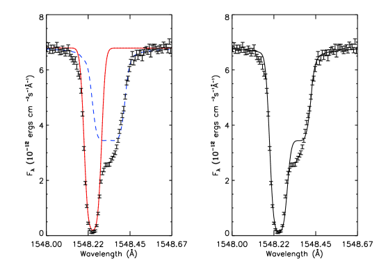
Figure 5: Addition of a Gaussian component (red solid line) to the photospheric (blue dashed line) component of C iv 1548Å. The left subplot shows the individual contributions to the absorption feature, while the right subplot shows the combined contribution from both lines. C iv/H=$2.13\times{10^{-7}}$. The discrepancy is explained in text.

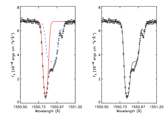
Figure 6: The same as Figure 5, but for the C iv 1550Å  line.

As well as the C iii lines listed in Table 10, the C iii resonant transition at 977.0201Å  (hereafter C iii 977Å) was available to fit, however, attempts to do so were unsuccessful, as the predicted profile could not descend deeply enough relative to the continuum, and increasing the C abundance resulted in large pressure broadening that was uncharacteristic of the observed profile. This does not come as a surprise, as the C iii 977Å  line has been observed along the line of sight to G191-B2B by Lehner et al. (2003) in the ISM. We attempted to add a Gaussian to account for this, but again, a satisfactory fit could not be obtained. Therefore, we determined the C iii abundance using only the lines in Table 10, obtaining C iii/H=$1.72_{-0.02}^{+0.02}\times{10^{-7}}$ (cf. Figure 7 for the C iii sextuplet).

Figure 7: Comparison between the model and observed spectra for the C iii sextuplet spanning 1174-1177Å  with C iii/H=$1.72\times{10^{-7}}$.

Our C iii and C iv abundances are in good agreement with Barstow et al. (2003b)’s C iii value of $1.99_{-0.88}^{+0.44}\times{10}^{-7}$, but not with their C iv value of $4.00_{-0.98}^{+0.44}\times{10}^{-7}$. We note, however, that Barstow et al. (2003b)’s C iv abundance was obtained without taking the circumstellar absorption into account. We also calculated the velocity of the circumstellar lines, obtaining $8.26_{-0.14}^{+0.18}$ and $8.30_{-0.15}^{+0.13}$ km s^-1 for the C iv 1548 and 1550Å  lines respectively, both in relatively good agreement with our obtained velocity corresponding to the Hyades Cloud velocity as identified by Redfield & Linsky (2008).

4.2 Nitrogen

Many N iv transitions exist in the FUSE spectrum of G191-B2B from 915-930Å, but we neglected using these lines in favour of N iv 1718.551Å  (hereafter N iv 1718Å) due to the higher S/N. We obtained N iv/H=$1.58_{-0.14}^{+0.14}\times{10^{-7}}$.

Using the resonant N v doublet lines at 1238.821 and 1242.804Å, we obtain N v/H=$2.16_{-0.04}^{+0.09}\times{10^{-7}}$. Our N iv abundance is in good agreement with that obtained by Barstow et al. (2003b) of $1.60_{-0.21}^{+0.41}\times{10^{-7}}$.

4.3 Oxygen

Absorption features of O iv-vi were detected in our line survey. Given the temperature of G191-B2B, the equivalent widths of the resonant O vi transitions (1031.93 and 1037.62Å) are quite weak, and were neglected from our analysis. Futhermore, attempts to obtain an abundance with the well known O v 1371.296Å  line were not possible. The predicted profile of the O v line did not appear in our synthesised spectrum unless O abundances of $\approx{10^{-6}}$ were specified. This issue may be related to that noted by Vennes et al. (2000), whereby the ionisation fraction for oxygen is poorly calculated for O iv/O v. Vennes et al. (2000) ruled out $T_{\mathrm{eff}}$ and log $g$ variations as being the cause, suggesting reasons such as additional atmospheric consituents, stratification, or inadequate model atom treatment. This is addressed in Vennes & Lanz (2001), whereby they used the O abundance determined from the O iv lines. This may also explain the large uncertainty in the O abundance value calculated by Barstow et al. (2003b) ($3.51_{-2.00}^{+7.40}\times{10^{-7}}$). Our abundance determination therefore is based only upon the O iv triplet listed in Table 10, whereby we found O iv/H=$4.12_{-0.08}^{+0.08}\times{10^{-7}}$, in good agreement with Barstow et al. (2003b).

4.4 Aluminium

Al was first observed in G191-B2B by Holberg et al. (1998) using IUE, however, an abundance was not calculated. Holberg et al. (2003), then considered the abundance of Al assuming LTE, arriving at an estimated value of $3.02\times{10}^{-7}$. We do not observe other isolated photospheric Al features. We obtained Al iii/H=$1.60_{-0.08}^{+0.07}\times{10^{-7}}$ (cf. Figure 8).

Figure 8: Comparison between the model (solid line) and observed (error bars) spectra for the Al iii 1854.716 (top plot) and 1862.79Å  (bottom plot) lines, with Al iii/H=$1.60\times{10^{-7}}$.

4.5 Silicon

For Si iii 1206.4995Å  (hereafter Si iii 1206Å), we were unable to fit the absorption feature as the predicted line profile did not descend deeply enough relative to the continuum. Increases in Si abundance produced a line profile that was pressure broadened far beyond that observed. Including a Gaussian into the fit, we obtained Si iii/H=$3.16_{-0.30}^{+0.31}\times{10^{-7}}$ (see Figure 9). We also determined the velocity of the Gaussian to be $9.24_{-0.06}^{+0.20}$ km s^-1. While we note that this velocity is not encompassed by the Hyades cloud velocity, the two values are quite close.

Holberg et al. (2003) noted an asymmetry in the absorption profiles of Si iv 1393.7546 and 1402.7697Å  (hereafter Si iv 1393Å  and 1402Å  respectively), observing a blue shifted component relative to the photospheric velocity. We confirmed this observation and included a Gaussian to account for its presence. We also included the excited Si IV transitions 1122.4849, 1128.3248, and 1128.3400Å  in order to further constrain the abundance. We derived Si iv/H=$3.68_{-0.14}^{+0.13}\times{10^{-7}}$. The velocities of the two Gaussians (see Figures 10 and 11) are $8.73_{-0.70}^{+0.93}$ and $8.31_{-1.39}^{+1.71}$ km s^-1 for the Si iv 1393 and 1402Ålines respectively, in good agreement with the Hyades cloud velocity. Both of our determined Si abundances are not encompassed by Barstow et al. (2003b)’s value of $8.65_{-3.50}^{+3.20}\times{10^{-7}}$, but the difference is not very large.

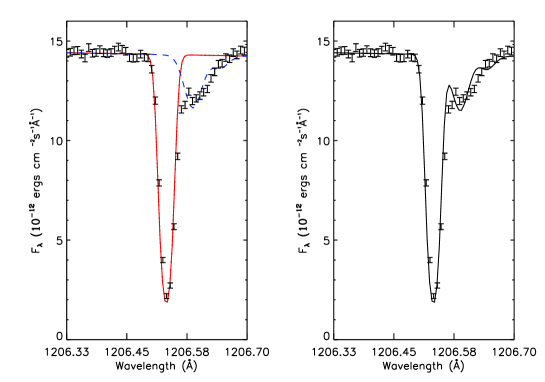
Figure 9: Addition of a Gaussian component (red solid line) to the photospheric (blue dashed line) Si iii 1206Å. The left subplot shows the individual contributions to the absorption feature, while the right subplot shows the combined contribution from both lines. Si iii/H=$3.16\times{10^{-7}}$.

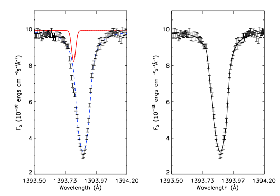
Figure 10: Same as Figure 9, but for the Si iv 1393Å  line with Si iv/H=$3.68\times{10^{-7}}$.

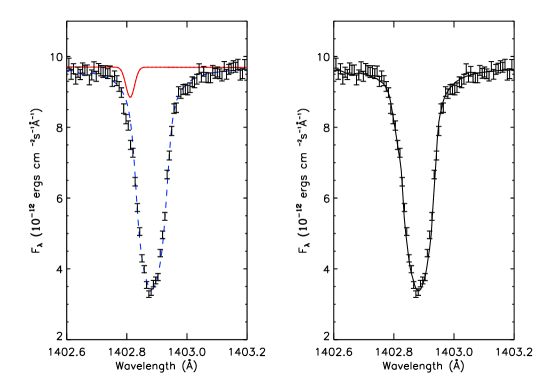
Figure 11: Same as Figure 10, but for the Si iv 1402Å  line.

4.6 Phosphorus

Resonance absorption features of P have been observed in a handful of DAs, including GD 394 (Chayer et al., 2000), GD 71, REJ 1918+595 and REJ 0605-482 (Dobbie et al., 2005). P was first observed in G191-B2B by Vennes et al. (1996) using the ORFEUS telescope, deriving an LTE abundance of $2.51_{-0.93}^{+1.47}\times{10^{-8}}$. Determination of the P iv abundance was complicated due to the proximity of the line to the Lyman $\gamma$ centroid, where the continuum varies rapidly with wavelength. We determined P iv/H=$8.40_{-1.18}^{+1.18}\times{10^{-8}}$ and P v/H=$1.64_{-0.02}^{+0.02}\times{10^{-8}}$. Our P v abundance appears to be in closer agreement with that obtained by Vennes et al. (1996).

4.7 Sulphur

This metal was also detected in G191-B2B by Vennes et al. (1996) with the ORPHEUS telescope, deriving an LTE abundance of S/H=$3.16_{-1.58}^{+3.15}\times{10^{-7}}$. We calculated S iv/H=$1.71_{-0.02}^{+0.02}\times{10^{-7}}$ and S vi=$5.23_{-0.13}^{+0.10}\times{10^{-8}}$. Our S iv abundance is also in agreement with Vennes et al. (1996).

4.8 Iron

While there have been many measurements of the Fe content in various white dwarf photospheric spectra (Barstow et al., 2003b; Vennes et al., 2006), none have used the same selection of lines, due to the large choice available. Here, we chose to use 12 strong lines for each ion listed in Table 10. We calculated Fe iv/H=$1.83_{-0.03}^{+0.03}\times{10^{-6}}$ and Fe v/H=$5.00_{-0.06}^{+0.06}\times{10^{-6}}$ (cf. Figure 12), with our Fe v abundance in agreement with Barstow et al. (2003b)’s value of $3.30_{-1.20}^{+3.10}\times{10^{-6}}$.

Figure 12: Comparison between the model (top line) and observed (bottom line) spectra for several Fe v lines, with Fe v/H=$5.00\times{10^{-6}}$. The synthetic spectrum is offset for clarity.

4.9 Nickel

Like Fe, Ni is a complicated atomic system with many transitions. We use a similar method to Fe to determine the abundance, obtaining Ni iv/H=$3.24_{-0.05}^{+0.13}\times{10^{-7}}$ and Ni v/H=$1.01_{-0.03}^{+0.03}\times{10^{-6}}$ (cf. Figure 13, where our Ni iv abundance agrees with Barstow et al. (2003b)’s value of $2.40_{-0.24}^{+0.84}\times{10^{-7}}$.

Figure 13: Comparison between the model (top line) and observed (bottom line) spectra for several Ni v lines, with Ni v/H=$1.01\times{10^{-6}}$. The synthetic spectrum is offset for clarity. The large absorption feature near 1239Å  is from N v.

5 Discussion

Our line survey has been successful in providing new line identifications, with over 95 percent of the absorption features detected in the STIS spectra and 100 percent of those in the FUSE data accounted for. Curiously, we confirmed the detection made by Vennes et al. (2005) of Ge iv, but we made no detections of heavier metals, or metals with atomic number between S and Fe.

In particular, we made no detections of Cr, Mn, or Co, for which Holberg et al. (2003) gave an abundance limit of $10^{-8}$. However, as highlighted in the previous section, some discrepancies still remain regarding predicted line profiles and ionisation balance for particular metals. In our discussion of the results, we first consider the metals where we have potentially identified circumstellar absorption features. Next, we discuss the calculated abundances of G191-B2B, and compare them to the solar abundances of Asplund et al. (2009), and the predicted abundances of Chayer et al. (1994); Chayer et al. (1995a); Chayer et al. (1995b) from radiative levitation calculations (cf. Figure 14). Finally, we consider the new atomic data, and the potential impact this may have on future model atmosphere calculations through the additional opacity that needs to be included.

5.1 Circumstellar absorption

As stated in section 4.1, the C iv 1548 and 1550Å  lines are accompanied by circumstellar absorption features which have been thoroughly documented. We have also confirmed the detection of circumstellar absorption in Si iv. The method of including a Gaussian to account for the circumstellar component is not new. Dickinson et al. (2012c) accounted for the line shape of the photospheric profile (which may include re-emission) as well as the circumstellar component, giving a more accurate representation of the absorption. However, our analysis of the profile allowed us to derive velocities and to make a comparison between the Hyades cloud and the circumstellar velocities.

Bannister et al. (2003) noted the similarity between the ISM and circumstellar velocities along the line of sight to G191-B2B, and suggested that the circumstellar lines arose from material ionised by the strömgren sphere of the white dwarf. Redfield & Linsky (2008) made the association between this ISM component with that of the Hyades cloud. This hypothesis was supported by Dickinson et al. (2012b)’s findings, and suggested that the Hyades cloud fell inside G191-B2B’s strömgren sphere. Our velocity measurements of the C iv and Si iv circumstellar features encompass the Hyades cloud velocity, and appear to support the strömgren sphere hypothesis. The velocity and uncertainty of the Si iii 1206Å  line does not quite encompass the Hyades cloud velocity. However, the discrepancy is small. So we can reasonably associate the Si iii line with the Hyades cloud. The issue of the C iii 977Å  line is more difficult owing to the low resolution of the data. While we can infer that there is additional absorption, we cannot derive any information about the absorption profile, and hence cannot derive a reliable velocity. The inability to fit a profile is most likely due to the resolution of the FUSE spectrometer.

5.2 General abundance discussion

With the exceptionally high S/N of the FUSE and STIS spectra, we have been able to constrain the formal $1\sigma$ uncertainties on most of the metal abundances to within a very small range. However, in reality, the true uncertainty on the abundances can be much greater than this due to a number of factors. As demonstrated by Figure 14, uncertainties in the ionisation balance can lead to order of magnitude differences in the calculated abundance from different ionisation stages. The ionic partition function, which is used to calculate the ionisation balance, is dependent on the atomic data of energy levels, and uncertain data can lead to incorrect calculations of level populations. It is interesting to note that in Figure 14, the largest difference between ionisation stage abundances was for P and S, where P iv/H and P v/H differ by $\sim{0.8}$ dex. The best agreement between ion abundances was for C and Si.

Figure 14: A comparison of abundances with respect to H for solar abundance (Asplund et al., 2009) (dotted line), atmospheric abundance as predicted from radiative levitation (dashed line) (Chayer et al., 1994; Chayer et al., 1995a; Chayer et al., 1995b), and the atmospheric abundances determined in our analysis (solid line). The error bars are omitted for clarity.

In Figure 14, we have plotted our measured abundances, comparing them to the solar abundances from Asplund et al. (2009), as well as the atmospheric abundances predicted by Chayer et al. (1994); Chayer et al. (1995a); Chayer et al. (1995b) due to radiative levitation. The only obvious agreement that can be observed in Figure 14 is between the radiative levitation prediction and our Fe v abundance. The largest discrepancy appears to be for Al, where radiative levitation grossly underestimates the abundance by more than two dex, this may, however, be due to the small number of bound-bound Al transitions included in the calculations.

5.3 Opacity considerations

The additional atomic data obtained for Fe and Ni has allowed all but a few lines to be identified. However, the number of heavy metal lines also presents a question regarding the efficacy of current methods in accounting for opacity in NLTE model atmosphere calculations. In Chayer et al. (1995a), the authors describe calculations performed to predict the abundance of Fe and Ni in the atmosphere of hot white dwarfs due to radiative levitation, and compared the Fe abundances predicted from using different atomic datasets from different generations (see Chayer et al. 1995a, Fig 11), concluding that the numbers of transitions, and the accuracy of their respective oscillator strengths varied the predicted Fe abundances. Such a result implies that using as complete a sample of transitions as possible is important in creating accurate models of radiative levitation. As shown in Table 5, the number of calculated transitions for Fe iv-vii alone in 1992 was $\sim{10^{7}}$, while for 2011 it was $\sim{10^{8}}$. Radiative transfer will also likely be affected by including the additional calculated lines. As described by Barstow et al. (1998), the inclusion of Fe and Ni transitions to a pure H atmosphere results in $T_{\mathrm{eff}}$ decreasing by a few thousand K. In terms of the SED, additional opacity may result in flux attenuation in the EUV, producing better agreement with observation. The additional opacity also potentially offers a solution to the Lyman-Balmer line problem. Barstow et al. (2003a) constructed two model grids with 0.1 and 10 times a nominal abundance, and measured $T_{\mathrm{eff}}$ and log $g$ for G191-B2B and REJ2214-492 using both the Lyman and Balmer line series. They found that the temperature discrepancy was larger for the lower abundance grid, and smaller for the higher grid. This implies that including additional opacity into future calculations may help to resolve the Lyman-Balmer line problem. To include the additional opacity contributed by the new lines, tlusty requires information on the energy levels, transitions, and photoionisation cross sections. tlusty is able to calculate bound-bound cross section directly from data provided by the Kurucz data, however, the photoionisation cross sections need to be included separately. Future work will involve calculations of the photoionisation cross sections. Our model atmospheres currently include 2,005,173 Fe iv-vi transitions, and 2,751,277 Ni iv-vi transitions. Future calculations therefore will include $\sim{30,000,000}$ Fe and $\sim{47,000,000}$ Ni transitions. This work not only has applications to white dwarf stars, but can also be applied to hot O and B stars.

6 Conclusions

We have presented the most detailed NUV and FUV spectroscopic survey of G191-B2B to date. Using all available high resolution observations with the E140H and E230H apertures with STIS, we have constructed a co-added spectrum whose S/N exceeds 100 in particular sections of the spectrum, and spans 1160-3145Å. The detail unveiled by such a high S/N spectrum far exceeds any observation of white dwarfs made thus far. Using the STIS spectrum, and the co-added FUSE spectrum from Barstow et al. (2010) covering 910-1185Å, we have made detections of 976 absorption features. By combining the latest releases of the Kurucz and Kentucky databases, we have been able to identify 947 of the detected features, blended or otherwise. We have identified every single absorption feature present in the FUSE spectrum of G191-B2B at our given confidence limit. We have found that over 60% of the identifications made can be attributed to highly ionised Fe and Ni features. While the new Fe and Ni features may be inaccurate in terms of their wavelengths and oscillator strengths, the high S/N STIS spectrum presents the opportunity to perform high quality measurements of atomic transition parameters in order to improve atomic databases.

Our survey confirmed the presence of previously observed circumstellar features and also potentially revealed a new, previously unconsidered Si iii circumstellar line.

Further, exploiting the high S/N data from the STIS and FUSE data, we have made highly accurate measurements of the abundances of metals present in G191-B2B’s photosphere. Our abundance analysis has revealed areas for improvement with regards to ionisation balance calculations. S and P appear to have the largest discrepancies.

We compared the calculated abundances from G191-B2B’s atmosphere to the solar photosphere, as well as predicted abundances due to radiative levitation. We highlighted the need for updated radiative levitation calculations using newly available atomic data in order to reconcile theory with observation.

We discussed the potential consequences of including new Fe and Ni transitions into NLTE model atmosphere calculations, as well as radiative levitation calculations. While the exact effect on the NLTE calculations cannot be quantified at present, we plan to perform a full, detailed investigation into the inclusion of new transitions in line blanketing calculations.

Appendix A Parameterisation of absorption features

The Gaussian and Lorentzian profiles fitted were parameterised respectively as:

$$F_{\lambda}=C_{1}\exp\left[-\frac{(\lambda-C_{2})^{2}}{2C_{3}^{2}}\right]$$ (3)

$$F_{\lambda}=\frac{C_{1}C_{3}^{2}}{(\lambda-C_{2})^{2}+C_{3}^{2}}$$ (4)

Where $C_{1}$, $C_{2}$ and $C_{3}$ are the height, centroid wavelength and line width respectively. The double Gaussian profile took the form:

$$F_{\lambda}=C_{1}\exp\left[-\frac{(\lambda-C_{2})^{2}}{2C_{3}^{2}}\right]+C_{4}\exp\left[-\frac{(\lambda-C_{5})^{2}}{2C_{6}^{2}}\right]$$ (5)

The $C_{i}$ are the same as defined for a single Gaussian. The Gaussian profile used in xspec was parameterised as:

$$F(E)=\exp\left[-\frac{\tau_{l}}{\sigma_{l}\sqrt{2\pi}}\exp\left[-\frac{(E-E_{l})^{2}}{2\sigma_{l}^{2}}\right]\right]$$ (6)

Where $E_{l}$ is the line energy in keV (line centroid), $\sigma$ is the line width (keV), and $\tau_{l}$ is the strength. This profile was multiplied by the model flux.

Appendix B Line identifications

Included here is a small excerpt of the table of identifications made in our survey. The table in its entirety can be found with the online version of the journal. Wavelengths and their associated errors are given in Å, equivalent width and error in mÅ, and velocities and errors in km s^-1. $\lambda_{\mathrm{obs}}$ and $\delta\lambda_{\mathrm{obs}}$, are the observed wavelength centroid and it’s error, and $\lambda_{\mathrm{lab}}$ and $\delta\lambda_{\mathrm{lab}}$ are the reference wavelength and, where available, the error on said wavelength. The velocity $v$ comes with two errors $\delta{v}$ and $\delta{v_{\mathrm{tot}}}$. The former is the error on the velocity assuming no error on the lab wavelength, and the latter takes all errors into account. The List column states where the transition data came from, with KENTUCKY=Kentucky database, KURUCZ=Kurucz database, NIST=NIST website, and RESONANT=V94. The Origin column states where the transition originated. Where PHOT=Photosphere, ISM1=Local Interstellar cloud, and ISM2=Hyades cloud. As was stated previously, many lines had several possible identifications, meaning that a line will be the result of several blends of absorption features. Therefore, where there was more than one identification, the characteristics of the measured line is given, followed only by the additional identifications and their velocities.

Table 13: List of detected Photospheric features from FUSE. Wavelengths ($\lambda$’s) are given in Å, wavelength errors in mÅ, equivalent widths in mÅ, and velocities in km s^-1. The full version of this table has been published online.

$\lambda_{\mathrm{obs}}$	$\delta\lambda_{\mathrm{obs}}$	$W_{\lambda}$	$\delta{W}_{\lambda}$	Ion	$\lambda_{\mathrm{lab}}$	$\delta\lambda_{\mathrm{lab}}$	$v$	$\delta{v}$	$\delta{v_{\mathrm{tot}}}$	List	Origin
916.503	0.533	168.903	2.369	H i	916.429	0.004	24.18	0.17	0.17	KENTUCKY	ISM1
917.254	0.600	170.652	2.643	H i	917.181	0.005	24.02	0.20	0.20	KENTUCKY	ISM1
918.196	0.574	196.800	2.500	H i	918.129	0.007	21.78	0.19	0.19	KENTUCKY	ISM1
918.964	7.564	10.266	2.198	N iv	918.893	7.500	23.16	2.47	3.48	KENTUCKY	PHOT
919.428	0.360	178.807	1.626	H i	919.351	0.009	25.00	0.12	0.12	KENTUCKY	ISM1
921.032	0.347	189.055	1.609	H i	920.963	0.012	22.45	0.11	0.11	KENTUCKY	ISM1
922.090	2.485	10.595	1.404	N iv	921.994	7.600	31.22	0.81	2.60	KENTUCKY	PHOT
922.607	2.409	10.460	1.358	N iv	922.519	7.600	28.60	0.78	2.59	KENTUCKY	PHOT
923.220	0.352	209.245	1.687	H i	923.150	0.016	22.64	0.11	0.11	KENTUCKY	ISM1
923.757	3.069	9.727	1.454	N iv	923.676	7.600	26.29	1.00	2.66	KENTUCKY	PHOT

References

- Arnaud (1996) Arnaud K. A., 1996, in Jacoby G. H., Barnes J., eds, Astronomical Data Analysis Software and Systems V Vol. 101 of Astronomical Society of the Pacific Conference Series, XSPEC: The First Ten Years. p. 17
- Asplund et al. (2009) Asplund M., Grevesse N., Sauval A. J., Scott P., 2009, in Blandford ed., Annual Review of Astronomy and Astrophysics, Vol. 47
- Bannister et al. (1999) Bannister N. P., Barstow M. A., Fraser G. W., Spragg J. E., Curddace R., Kowalski M., Fritz G., Yentis D., Lapington J., Tandy J., Sanderson B., Barbee T., Goldstein W. H., Kordas 1999, in Solheim S. E., Meistas E. G., eds, 11th European Workshop on White Dwarfs Vol. 169 of Astronomical Society of the Pacific Conference Series, The Joint Astrophysical Plasmadynamic Experiment (JPEX). p. 188
- Bannister et al. (2003) Bannister N. P., Barstow M. A., Holberg J. B., Bruhweiler F. C., 2003, MNRAS, 341, 477
- Barstow et al. (2010) Barstow M. A., Boyce D. D., Welsh B. Y., Lallement R., Barstow J. K., Forbes A. E., Preval S., 2010, ApJ, 723, 1762
- Barstow et al. (2005) Barstow M. A., Cruddace R. G., Kowalski M. P., Bannister N. P., Yentis D., Lapington J. S., Tandy J. A., Hubeny I., Schuh S., Dreizler S., Barbee T. W., 2005, MNRAS, 362, 1273
- Barstow et al. (2003a) Barstow M. A., Good S. A., Burleigh M. R., Hubeny I., Holberg J. B., Levan A. J., 2003, MNRAS, 344, 562
- Barstow et al. (2003b) Barstow M. A., Good S. A., Holberg J. B., Hubeny I., Bannister N. P., Bruhweiler F. C., Burleigh M. R., Napiwotzki R., 2003, MNRAS, 341, 870
- Barstow et al. (1998) Barstow M. A., Hubeny I., Holberg J. B., 1998, MNRAS, 299, 520
- Barstow et al. (1999) Barstow M. A., Hubeny I., Holberg J. B., 1999, MNRAS, 307, 884
- Bergeron et al. (1995) Bergeron P., Liebert J., Fulbright M. S., 1995, ApJ, 444, 810
- Bergeron et al. (2011) Bergeron P., Wesemael F., Dufour P., Beauchamp A., Hunter C., Saffer R. A., Gianninas A., Ruiz M. T., Limoges M. M., Dufour P., Fontaine G., Liebert J., 2011, ApJ, 737, 28
- Bohlin & Gilliland (2004) Bohlin R. C., Gilliland R. L., 2004, AJ, 127, 3508
- Bruhweiler & Kondo (1981) Bruhweiler F. C., Kondo Y., 1981, ApJL, 248, L123
- Bruhweiler et al. (1999) Bruhweiler F., Barstow M., Holberg J., Sahu M., 1999, in American Astronomical Society Meeting Abstracts Vol. 31 of Bulletin of the American Astronomical Society, The Unusual C IV Absorption in the Spectrum of the DA White Dwarf G191-B2B. p. 1419
- Chayer et al. (1995a) Chayer P., Fontaine G., Wesemael F., 1995, ApJS, 99, 189
- Chayer et al. (2000) Chayer P., Kruk J. W., Ake T. B., Dupree A. K., Malina R. F., Siegmund O. H. W., Sonneborn G., Ohl R. G., 2000, ApJL, 538, L91
- Chayer et al. (1994) Chayer P., LeBlanc F., Fontaine G., Wesemael F., Michaud G., Vennes S., 1994, ApJL, 436, L161
- Chayer et al. (1995b) Chayer P., Vennes S., Pradhan A. K., Thejll P., Beauchamp A., Fontaine G., Wesemael F., 1995, ApJ, 454, 429
- Cruddace et al. (2002) Cruddace R. G., Kowalski M. P., Yentis D., Brown C. M., Gursky H., Barstow M. A., Bannister N. P., Fraser G. W., Spragg J. E., Lapington J. S., Tandy J. A., Sanderson B., Culhane J. L., Barbee T. W., Kordas J. F., Goldstein W., Fritz G. G., 2002, ApJL, 565, L47
- Dickinson et al. (2012b) Dickinson N. J., Barstow M. A., Hubeny I., 2012, MNRAS, 421, 3222
- Dickinson et al. (2012c) Dickinson N. J., Barstow M. A., Welsh B. Y., 2012, MNRAS, 428, 1873
- Dickinson et al. (2012a) Dickinson N. J., Barstow M. A., Welsh B. Y., Burleigh M., Farihi J., Redfield S., Unglaub K., 2012, MNRAS, 423, 1397
- Dixon et al. (2007) Dixon W. V., Sahnow D. J., Barrett P. E., Civeit T., Dupuis J., Fullerton A. W., Godard B., Hsu J. C., Kaiser M. E., Kruk J. W., Lacour S., Lindler D. J., Massa D., Robinson R. D., Romelfanger M. L., Sonnentrucker P., 2007, PASP, 119, 527
- Dobbie et al. (2005) Dobbie P. D., Barstow M. A., Hubeny I., Holberg J. B., Burleigh M. R., Forbes A. E., 2005, MNRAS, 363, 763
- Dreizler & Wolff (1999) Dreizler S., Wolff B., 1999, AAP, 348, 189
- Eggen & Greenstein (1967) Eggen O. J., Greenstein J. L., 1967, ApJ, 150, 927
- Good et al. (2004) Good S. A., Barstow M. A., Holberg J. B., Sing D. K., Burleigh M. R., Dobbie P. D., 2004, MNRAS, 355, 1031
- Greenstein (1969) Greenstein J. L., 1969, ApJ, 158, 281
- Hernandez (2012) Hernandez, S., et al. 2012, ”STIS Instrument Handbook”, Version 12.0, (Baltimore: STScI)
- Holberg et al. (1985) Holberg J. B., Wesemael F., Wegner G., Bruhweiler F. C., 1985, ApJ, 293, 294
- Holberg et al. (1994) Holberg J. B., Hubeny I., Barstow M. A., Lanz T., Sion E. M., Tweedy R. W., 1994, ApJL, 425, L105
- Holberg et al. (1998) Holberg J. B., Barstow M. A., Sion E. M., 1998, ApJS, 119, 207
- Holberg et al. (1999) Holberg J. B., Barstow M. A., Sion E. M., 1999, in Solheim S. E., Meistas E. G., eds, 11th European Workshop on White Dwarfs Vol. 169 of Astronomical Society of the Pacific Conference Series, Elemental abundances in hot white dwarfs. p. 485
- Holberg et al. (2002) Holberg J. B., Barstow M. A., Hubeny I., Sahu M. S., Bruhweiler F. C., Landsman W. B., 2002, in American Astronomical Society Meeting Abstracts #200 Vol. 34 of Bulletin of the American Astronomical Society, A High S/N View of the Photosphere of the Hot White Dwarf G191-B2B from STIS. p. 765
- Holberg et al. (2003) Holberg J. B., Barstow M. A., Hubeny I., Sahu M. S., Bruhweiler F. C., Landsman W. B., 2003 Vol. 291 of ASPCS, A Detailed View of the Photosphere of the Hot White Dwarf G191-B2B from STIS. p. 383
- Holberg & Bergeron (2006) Holberg J. B., Bergeron P., 2006, AJ, 132, 1221
- Hubeny (1988) Hubeny I., 1988, Computer Physics Communications, 52, 103
- Hubeny & Lanz (2011) Hubeny I., Lanz T., 2011, in Astrophysics Source Code Library, record ascl:1109.022 Synspec: General Spectrum Synthesis Program. p. 9022
- Kahn et al. (1984) Kahn S. M., Wesemael F., Liebert J., Raymond J. C., Steiner J. E., Shipman H. L., 1984, ApJ, 278, 255
- Kowalski & Saumon (2006) Kowalski P. M., Saumon D., 2006, ApJL, 651, L137
- Kurucz (1992) Kurucz R. L., 1992, RMxAA, 23, 45
- Kurucz (2006) Kurucz R. L., 2006, in Stee P., ed., EAS Publications Series Vol. 18 of EAS Publications Series, Including all the Lines. pp 129–155
- Kurucz (2011) Kurucz R. L., 2011, Canadian Journal of Physics, 89, 417
- Lajoie & Bergeron (2007) Lajoie C. P., Bergeron P., 2007, ApJ, 667, 1126
- Lanz et al. (1996) Lanz T., Barstow M. A., Hubeny I., Holberg J. B., 1996, ApJ, 473, 1089
- Lehner et al. (2003) Lehner N., Jenkins E. B., Gry C., Moos H. W., Chayer P., Lacour S., 2003, ApJ, 595, 858
- Markwardt (2009) Markwardt C. B., 2009, in Bohlender D. A., Durand D., Dowler P., eds, Astronomical Data Analysis Software and Systems XVIII Vol. 411 of Astronomical Society of the Pacific Conference Series, Non-linear Least-squares Fitting in IDL with MPFIT. p. 251
- Moos (2000) Moos H. W. et al, 2000, ApJL, 538, L1
- Oke (1974) Oke J. B., 1974, ApJS, 27, 21
- Redfield & Linsky (2008) Redfield S., Linsky J. L., 2008, ApJ, 673, 283
- Reid & Wegner (1988) Reid N., Wegner G., 1988, ApJ, 335, 953
- Sahnow (2000) Sahnow D. J. et al, 2000, ApJL, 538, L7
- Sion et al. (1992) Sion E. M., Bohlin R. C., Tweedy R. W., Vauclair G. P., 1992, ApJL, 391, L29
- Tremblay et al. (2011) Tremblay P. E., Bergeron P., Gianninas A., 2011, ApJ, 730, 128
- Vennes et al. (1996) Vennes S., Chayer P., Hurwitz M., Bowyer S., 1996, ApJ, 468, 898
-
Vennes et al. (2000)
Vennes S., Polomski E. F., Lanz T., Thorstensen J. R., Chayer P.,
Gull T. R., 2000,
apj, 544, 423 - Vennes & Lanz (2001) Vennes S., Lanz T., 2001, ApJ, 553, 399
- Vennes et al. (2005) Vennes S., Chayer P., Dupuis J., 2005, ApJL, 622, L121
- Vennes et al. (2006) Vennes S., Chayer P., Dupuis J., Lanz T., 2006, ApJ, 652, 1554
- Verner et al. (1994) Verner D. A., Barthel P. D., Tytler D., 1994, A&A, 108, 287
- Werner & Dreizler (1994) Werner K., Dreizler S., 1994, AAP, 286, L31
- Wood (1998) Wood M. A., 1998, Highlights of Astronomy, 11, 427