The effects of thermodynamic stability on wind properties in different low mass black hole binary states

Abstract

We present a systematic theory-motivated study of the thermodynamic stability condition as an explanation for the observed accretion disk wind signatures in different states of low mass black hole binaries (BHB). The variability in observed ions is conventionally explained either by variations in the driving mechanisms or the changes in the ionizing flux or due to density effects, whilst thermodynamic stability considerations have been largely ignored. It would appear that the observability of particular ions in different BHB states can be accounted for through simple thermodynamic considerations in the static limit. Our calculations predict that in the disk dominated soft thermal and intermediate states, the wind should be thermodynamically stable and hence observable. On the other hand, in the powerlaw dominated spectrally hard state the wind is found to be thermodynamically unstable for a certain range of $3.55\leq\log\xi\leq 4.20$. In the spectrally hard state, a large number of the He-like and H-like ions (including e.g. Fe  xxv, Ar  xviii and S  xv have peak ion fractions in the unstable ionization parameter ($\xi$) range, making these ions undetectable. Our theoretical predictions have clear corroboration in the literature reporting differences in wind ion observability as the BHBs transition through the accretion states (Lee et al., 2002; Miller et al., 2008; Neilsen & Lee, 2009; Blum et al., 2010; Ponti et al., 2012; Neilsen & Homan, 2012). While this effect may not be the only one responsible for the observed gradient in the wind properties as a function of the accretion state in BHBs, it is clear that its inclusion in the calculations is crucial to understanding the link between the environment of the compact object and its accretion processes.

1 Introduction

Most stellar mass black hole binaries (BHBs) show common behaviour patterns centered around a few states of accretion. The different accretion states are signified by different spectral energy distributions (among other things) having varying degree of contribution from the accretion disk and the non-thermal powerlaw components. In addition, since Chandra and XMM-Newton, there has been increased interest in winds from the accretion disk, as a result of detections of blueshifted absorption lines of varying velocities and temperatures, seen in high resolution X-ray spectra. In order to get a consolidated picture of these systems, it is necessary to understand the relation between the accretion states of the BHBs and the properties of the accretion disk winds.

The Chandra HETGS (High Energy Transmission Grating Spectrometer, Canizares et al. 2005) sensitive 0.5-7.5 keV energy range is rich in atomic transitions. Yet often absorption lines from only H- and He-like Fe are detected (e.g Lee et al. 2002, Neilsen & Lee 2009 for GRS 1915+105, Miller et al. 2004 for GX 339-4, Miller et al. 2006 for H1743-322 and King et al. 2012 for IGR J17091-3624). On the other hand in some rare cases a range of ions is seen, from O through Fe (e.g. Ueda et al. 2009 for GRS 1915+105, Miller et al. 2008; Kallman et al. 2009 for GRO J1655–40). This suggests that the wind properties, e.g. temperature and density, may vary depending on the source and/or the accretion state. In this paper we restrict our discussion to low mass BHBs to ensure that wind signatures originate from the accretion disk rather than from the stellar companion (as in the case of high mass X-ray binaries). However, we note that accretion disk winds are detected in neutron star binary systems as well (e.g Brandt & Schulz 2000, Schulz & Brandt 2002 for Cir X-1, Ueda et al. 2004 for GX 13+1, Reynolds & Miller 2010 for 1A0535+262 and Miller et al. 2011 for IGR J17480-2446) and that some high mass X-ray binaries (where the companion to the compact object is a high mass star) exhibit stellar winds diagnosed through emission (e.g. Vela X-1, Schulz et al. 2002; LMC X-4, Neilsen et al. 2009) or absorption (e.g. Cyg X-1, Hanke et al. 2009).

X-ray studies of BHBs show that winds are not present in all states. Neilsen & Lee (2009) demonstrated that the equivalent width of the Fe XXVI absorption line is anti-correlated with the fractional hard power law contribution to the spectrum in GRS 1915+105: the softer the state, the more prominent the absorption lines; see also Miller et al. (2008); Blum et al. (2010). Recently a confirmation of this finding came from the Ponti et al. (2012) compilation of wind results (by the aforementioned and other authors) verifying the state dependent nature of accretion disk winds in general.

As an explanation for the observed changes in these winds, authors have commonly invoked differences in photoionizing flux (e.g. Miller et al., 2012, for H1743-322). However, since the properties of winds are also a result of their driving mechanisms (Lee et al., 2002; Ueda et al., 2009, 2010; Neilsen et al., 2011; Neilsen & Homan, 2012), observed wind variations may also indicate changes in these driving mechanisms. For example, a well known Chandra observation of GRO J1655–40 (Miller et al., 2006, 2008; Kallman et al., 2009), showing a rich absorption line spectrum with ions from OVIII to NiXXVI. Miller et al. (2006, 2008) argue in favour of the magnetic driving mechanism for the wind. But a Chandra observation from 3 weeks earlier, for the same object, shows only Fe  xxvi absorption (Neilsen & Homan, 2012). The changes cannot be explained by changes in the photoionizing flux alone, and Neilsen & Homan (2012) suggest that variable thermal pressure and magnetic fields may both be important in driving long-term changes in this wind.

Interestingly while changes in the photoionizing flux, in the driving mechanisms and in the wind density are frequently invoked to explain the observed wind behaviour, the thermodynamic stability of these outflows its relevance to the detectability of particular ions in BHBs have never been discussed in detail. Although quite commonly used for assessing winds in active galactic nuclei (Krolik et al., 1981; Reynolds & Fabian, 1995; Hess et al., 1997; Chakravorty et al., 2009, 2012; Lee et al., 2013), thermodynamic stability arguments have not been used much to explain observed BHB wind behaviour. (However, see Jimenez-Garate et al. 2002 for a specific use of the stability curves for determining accretion disk atmosphere properties for neutron star binaries.) Using thermal equilibrium curves, in this paper we test the importance of thermodynamic stability for the observable properties of winds in different accretion states of BHBs. We are particularly interested in testing if the prevalence of the winds in the softer states (as noted by Neilsen & Lee, 2009; Ponti et al., 2012, etc.) can be explained using thermodynamic stability arguments.

2 The Spectral Energy Distribution

We begin our considerations by adopting appropriate spectral energy distributions (SEDs) for different BHB states. The SED of BHBs usually contains, to varying degrees, (1) a thermal component conventionally modeled with a multi-temperature blackbody originating from the inner accretion disk and often showing a characteristic temperature ($T_{in}$) near 1 keV and (2) a non thermal power-law component with a photon spectrum $N(E)\propto E^{-\Gamma}$ (Remillard & McClintock, 2006). The thermal state is dominated by the radiation from the inner accretion disk contributing more than 75% of the 2-20 keV flux (e.g. dashed red line on top panel of Figure 1). In contrast the hard power law state (a.k.a. hard state; solid black line in Figure 1) is dominated by a flat power law component ($\Gamma\sim 1.8$) that contributes more than 80% of the 2-20 keV flux. For any given BHB, the accretion disk usually appears to be fainter and cooler in this hard power law state than it is in the thermal state.

The radiation from a thin accretion disk may be modeled as the sum of local blackbodies emitted at different radii. A simple prescription for the radial distribution of the temperature is:

$$T(R)=6.3\times 10^{5}\left(\frac{\dot{m}}{\dot{m}_{\rm Edd}}\right)^{\frac{1}{4}}\left(\frac{M_{\rm{BH}}}{10^{8}M_{\odot}}\right)^{-\frac{1}{4}}\left(\frac{R}{R_{s}}\right)^{-\frac{3}{4}}\rm{K}$$ (1)

(Peterson, 1997; Frank, King & Raine, 2002) where $\dot{m}$ is the accretion rate of the central black hole of mass $M_{\rm{BH}}$, $\dot{m}_{\rm Edd}$ is its Eddington accretion rate and $R_{s}=2GM_{\rm{BH}}/c^{2}$ is the Schwarzschild radius ($G$ is the gravitational constant and $c$ is the velocity light). To describe the radiation from the accretion disk $f_{disk}(\nu)$, we use the Zimmerman (2005) model ezdiskbb (from XSPEC, Arnaud 1996). The model ezdiskbb imposes the physical boundary condition that the viscous torque should be zero at the inner edge of the disk at radius $R_{in}$. The model is parametrised by

$$T_{max}=0.488fT_{in}=0.488fT(R_{in})$$ (2)

and

$$A_{ezdbb}=\left(1/f^{4}\right)\left\{\frac{R_{in}/\rm{km}}{D/(10\,\,\rm{kpc})}\right\}^{2}\cos\theta$$ (3)

where Equation 1 is used to calculate $T(R_{in})$; $D$ is the distance of the source from us, $\theta$ is the angle that our line-of-sight makes to the normal to the disc plane; $f$ is the hardening factor which accounts for the modification of the optically thick disk emission from a pure blackbody. We use the established value $f=1.7$ (Shimura & Takahara, 1995)

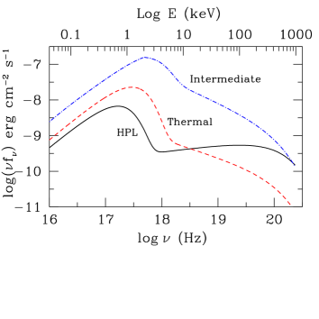
Figure 1: The SEDs for the three different accretion states of a black hole of mass $7M_{\odot}$ at a distance of 5 kpc from us. The two SED components (disk and powerlaw) are added following the schemes described in Remillard & McClintock (2006). See Section 2 for the details.

We add a power-law component to the disk spectrum using

$$f(\nu)=f_{disk}(\nu)+[A_{pl}\nu^{-\alpha}]\exp{{}^{-\frac{\nu}{\nu_{max}}}}$$ (4)

to account for the full BHB SED, where $\alpha=\Gamma-1$ is the spectral index of the powerlaw.

In their review, Remillard & McClintock (2006) used the different SEDs of the 1996-97 outburst of the BHB GRO J1655–40 (hereafter GROJ1655, Sobczak et al., 1999; Orosz et al., 1997) to demonstrate the SEDs of a typical BHB in its different states. Following their prescription, we define three different fiducial SEDs for the three states of a $7M_{\odot}$ black hole at a distance of 5 kpc from us. (Note that the the distance of the black hole from us does not have any consequence on the thermodynamic calculations presented in this paper for the absorbing gas which is very close to the black hole. To determine the photoionization state of the gas, it is sufficient to know the shape of the SED and the ionization parameter. Thus the exact value of the distance is not important.) We also find in Section 4.1.1 that a variation in $4M_{\odot}\leq M_{\rm{BH}}\leq 15M_{\odot}$ does not strongly affect our overall conclusions.) Subsequent results presented in this paper will be based on the following SED definitions we adopt for the three typical low mass BHB states.

1. Thermal state (Figure 1 dashed red curve): To generate the disk spectrum, we choose $\left(\dot{m}/\dot{m}_{\rm Edd},R_{in}/R_{s}\right)=(0.2,6.0)$ resulting in $T_{max}$ ($T_{in}$) = 0.48 (0.58)  keV. The powerlaw has $\Gamma=2.5$ and $A_{pl}$ is chosen in such a way that the 2-20 keV disk flux contribution $f_{d}=0.8$.

2. Intermediate state (Figure 1 dotted blue curve): The disk spectrum is generated with $\left(\dot{m}/\dot{m}_{\rm Edd},R_{in}/R_{s}\right)=(0.4,3.0)$ so that $T_{max}$ ($T_{in}$) = 0.97 (1.17)  keV. For the powerlaw, $\Gamma=2.7$ and $f_{d}=0.5$.

3. Hard powerlaw (hereafter HPL) state (Figure 1 solid black curve): With $\left(\dot{m}/\dot{m}_{\rm Edd},R_{in}/R_{s}\right)=(0.1,10.0)$ we generate a cooler disk with $T_{max}$ ($T_{in}$) = 0.28 (0.33)  keV. The powerlaw is dominant in this state with $\Gamma=1.8$ and $f_{d}=0.2$.

For each of the SEDs defined above, we use a high energy exponential cut-off (Equation 4) to insert a break in the power law at $E_{b}=100$ keV (Figure 1). See Section 4.1.3 for a discussion of the effects of varying $E_{b}$. (In soft states $E_{b}$ can be less than 20 keV, and we accommodate this in our considerations of thermodynamic stability for soft states; see Section 4.1.3 for details.)

Note that even though we base BHB state SEDs on GRO J1655 (following Remillard & McClintock, 2006), our results are intended to be generic to stellar mass black holes (in so far as the 1996-97 outburst of GRO J1655 was representative of a typical BHB outburst). We use these SEDs as reasonable representations of the ionizing spectra for different BHB states, and we use similar representative parameters for the wind properties (e.g. density, column density, and metallicity). In subsequent sections, we make quantitative tests of the influence of these choices, and find that our results are robust to changes in the SED and wind properties (including $M,\,\,\dot{m}\,\,\rm{and}\,\,R_{in}$ in Section 4.1.1; $f_{d}$ and $\Gamma$ and in Section 4.1.3; $E_{b}$ in Section 4.1.3 and wind density in Section 4.2.

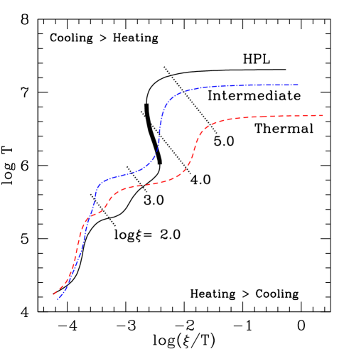
Figure 2: Stability curves for photoionised Solar metallicity gas with density $n_{\rm H}=10^{14}\rm{cm^{-3}}$ and column density $N_{\rm H}=10^{23}\rm{cm^{-2}}$. The different curves correspond to the three different ionizing continuum for the three different accretion states of the black hole, described in Figure 1 and Section 2. The dotted black lines cutting across the stability curves mark regions of constant $\xi$, also demonstrating the range of $\xi$ spanned by the stability curves. The highlighted region (thick black line) of the stability curve for the HPL state shows the range of thermodynamically unstable phases. The other two stability curves are stable throughout.

3 Photoionization calculations for thermodynamic equilibrium

In this Section we use the aforementioned (Figure 1; Section 2) ionizing SEDs for the different BHB states to calculate the expected temperature, pressure (Section 3.1) of the outflowing gas, and the ionization fractions (Section 3.2) of the various ions in the gas. This will allow us to assess the thermodynamic stability of winds as a means of explaining the presence/absence of observable ionic species in different BHB states.

$\log\xi$		HPL			Thermal			Intermediate
		Heating	Cooling		Heating	Cooling		Heating	Cooling
					$n_{\rm H}=10^{6}\rm{cm^{-3}}$
		aHI, n=2 (25.7)	bH iso. of H (42.1)		HI, n=2 (24.4)	H iso. of H (35.6)		HI, n=2 (21.1)	H iso. of H (23.3)
		HeI (18.2)	FeII recomb.c (20.4)		OI (15.8)	FeII recomb. (22.0)		OI (18.1)	FeII recomb. (23.2)
		OII (12.9)	MgII 2795.5 $\AA$ (6.0)		HeI (11.5)	MgII 2795.5 $\AA$ (5.8)		FeII (10.1)	FeII recomb. (9.9)
					$n_{\rm H}=10^{10}\rm{cm^{-3}}$
		OII (30.2)	H iso. of H (33.7)		OII (28.0)	H iso. of H (49.9)		OII (20.7)	H iso. of H (55.0)
0.0		HeI (27.4)	MgII 2795.5 $\AA$ (15.7)		HeI (15.3)	Free-free (13.5)		HeI (10.7)	Free-free (15.6)
		CII (7.5)	MgII 2802.7$\AA$ (10.6)		NeII (6.6)	MgII 2795.5 $\AA$ (11.5)		FeII (9.1)	MgII 2795.5 $\AA$ (8.3)
					$n_{\rm H}=10^{14}\rm{cm^{-3}}$
		O II (25.5)	H recomb. (33.0)		O II (27.4)	H recomb. (33.0)		O II (25.2)	H recomb. (32.9)
		H I (15.5)	Free-free (26.4)		H I (11.8)	Free-free (27.2)		H I (12.8)	Free-free (24.2)
		He II (15.2)	H iso. of H (19.6)		Fe III (11.3)	H iso. of H (19.0)		Fe III (11.5)	H iso. of H (23.8)
					$n_{\rm H}=10^{6}\rm{cm^{-3}}$
		HeII (49.6)	CIV 1548$\AA$ (13.0)		HeII (33.7)	CIV 1548$\AA$ (17.6)		HI (28.6)	H iso. of H (46.9)
		OIV (10.2)	OIII 5007$\AA$ (8.1)		OIV (11.1)	OIII 5007$\AA$ (9.1)		OIII (17.0)	OIII 5007$\AA$ (12.7)
		OIII (7.7)	CIV 1551$\AA$ (6.5)		OIII (10.3)	CIV 1551$\AA$ (8.8)		HeII (10.5)	CIII 1910$\AA$ (8.6)
					$n_{\rm H}=10^{10}\rm{cm^{-3}}$
		HeII (40.2)	CIV 1548$\AA$ (32.3)		HeII (25.4)	CIV 1548$\AA$ (30.9)		OII (25.7)	Si III 1892$\AA$ (16.5)
1.0		OIV (11.0)	CIV 1551$\AA$ (17.2)		OIII (14.7)	CIV 1551$\AA$ (16.7)		SiIII (6.7)	CII 1335$\AA$ (14.5)
		OIII (10.6)	CIII 977$\AA$ (4.4)		OIV (10.6)	CIII 977$\AA$ (7.3)		FeIII (6.6)	H iso. of H (12.0)
					$n_{\rm H}=10^{14}\rm{cm^{-3}}$
		O V (21.9)	Free-free (20.2)		O V (22.1)	Free-free (15.3)		O IV (16.2)	Free-free (12.0)
		O IV (18.2)	H recomb. (13.4)		O IV (15.8)	H recomb. (9.7)		O III (15.4)	H recomb. (8.5)
		Ne V (6.3)	H iso. of H (10.0)		Ne V (7.6)	H iso. of H (6.5)		Ne IV (6.7)	H iso. of He (6.7)
					$n_{\rm H}=10^{6}\rm{cm^{-3}}$
		HeII (17.2)	Free-free (19.8)		OVIII (16.1)	Free-free (25.4)		OVIII (13.9)	Free-free (23.1)
		OVIII (11.5)	SiXII 499$\AA$ (5.6)		HeII (15.4)	H iso. of He (14.3)		FeXVIII (9.6)	H iso. of He (18.3)
		FeXIV (7.1)	H recomb. (5.6)		FeXVIII (7.7)	H recomb. (10.3)		FeXIX (8.3)	H recomb. (5.4)
					$n_{\rm H}=10^{10}\rm{cm^{-3}}$
		HeII (16.0)	Free-free (20.4)		OVIII (16.4)	Free-free (25.8)		OVIII (13.9)	Free-free (23.1)
2.0		OVIII (11.6)	FeXV 284.2$\AA$ (6.1)		HeII (14.2)	H iso. of He (13.3)		FeXVIII (9.6)	H iso. of He (17.7)
		FeXIV (7.5)	SiXII 499$\AA$ (6.0)		FeXVIII (8.0)	H recomb. (6.5)		FeXIX (8.1)	H recomb. (5.5)
					$n_{\rm H}=10^{14}\rm{cm^{-3}}$
		O VIII (15.8)	Free-free (22.1)		O VIII (20.0)	Free-free (25.2)		O VIII (17.7)	Free-free (24.6)
		He II (7.8)	H recomb. (9.4)		Fe XVIII (9.1)	H recomb. (9.5)		Fe XIX (12.1)	H iso. of He (8.8)
		Fe UTAd (7.4)	He recomb. (6.7)		Fe XIX (9.0)	H iso. of He (7.8)		Fe XVIII (8.9)	H recomb. (7.7)
					$n_{\rm H}=10^{14}\rm{cm^{-3}}$
		Fe XX (14.9)	Compton (43.0)		Fe XXII (14.4)	Free-free (39.7)		Fe XXIII (14.1)	Free-free (46.0)
3.0		Compton (13.3)	H recomb. (9.3)		O VIII (14.4)	H recomb. (8.6)		O VIII (14.0)	Fe XXIV - 192 Å(7.8)
		Fe XIX (11.5)	He recomb. (9.2)		Fe XXI (13.8)	He recomb. (8.5)		Fe XXII (9.8)	He recomb. (7.8)
					$n_{\rm H}=10^{14}\rm{cm^{-3}}$
		Compton (79.2)	Free-free (69.1)		Compton (35.7)	Free-free (60.4)		Compton (62.5)	Free-free (69.8)
4.0		Fe XXV (6.3)	Compton (16.0)		O VIII (11.8)	He recomb. (10.0)		Fe XXV (10.5)	Compton (13.0)
		Fe XXIV (2.1)	He recomb. (3.8)		Fe XXIV (11.1)	H recomb. (8.7)		O VIII (4.8)	He recomb. (5.4)
					$n_{\rm H}=10^{14}\rm{cm^{-3}}$
		Compton (98.3)	Compton (82.0)		Compton (88.1)	Compton (66.0)		Compton (9.7)	Compton (77.4)
5.0		Fe XXVI (1.0)	Free-free (16.6)		Fe XXV (3.8)	Free-free (28.1)		Fe XXVI (1.8)	Free-free (20.2)
		Fe XXV (0.1)	Fe XXV recomb. (0.3)		Fe XXVI (3.1)	He recomb. (1.8)		O VIII (0.2)	Fe XXV recomb. (0.5)

^a HI, n=2 —$>$ photoionization from the n=2 level of neutral Hydrogen

^b H iso. —$>$ Hydrogen iso-sequence

^c recomb. —$>$ recombination

^d UTA —$>$ Unresolved transition array (2p-3d inner-shell absorption by iron M-shell ions)

Table 1: The heating and cooling agents as a function of $\log\xi$ for the HPL, thermal and intermediate stability curves. For $\log\xi\leq 2.0$ we have listed the agents for three different densities $n_{\rm H}=10^{6},10^{10}\,\,\rm{and}\,\,10^{14}\rm{cm^{-3}}$, whereas for higher ionization parameters (which are insensitive to density variations; see Section 4.2) we have given the list for only $n_{\rm H}=10^{14}\rm{cm^{-3}}$. The numbers in the parentheses give the fractional heating or cooling contributed (in percentage) by the particular agent. We have listed only the top three contributing agents in each case. When a given ion is listed as the heating agents it is its photoionization which is responsible for heating the gas.

3.1 Stability curves

Thermodynamic stability of photoionized gas can be studied effectively using the thermal equilibrium curve of the temperature ($T$) versus the pressure ($\xi/T$) of the gas (Krolik et al., 1981; Reynolds & Fabian, 1995; Hess et al., 1997; Chakravorty et al., 2008, 2009, 2012; Lee et al., 2013); here $\xi=L/n_{\rm H}r^{2}$ is the ionization parameter. Along the stability curve, heating and cooling are balanced everywhere, but gas in thermal equilibrium is only thermodynamically stable where the slope of the curve is positive. The thermodynamic stability of the photoionized gas is determined by the balance of the major heating and cooling mechanisms along the curves (see Table 1 for an example list of such agents, varying with $\xi$). We expect that if the photoionized gas (as diagnosed through observed absorption lines) is detected, its ionization parameter is such that the gas is in thermal equilibrium. Hence the $\xi/T-T$ point of such gas should lie on the stable parts of the stability curve.

We model the photoionized absorber as an optically thin, plane parallel slab of Solar metallicity (Allende Prieto et al., 2001, 2002; Holweger, 2001; Grevesse & Sauval, 1998) gas with density $n_{\rm H}=10^{14}\rm{cm^{-3}}$ and column density $N_{\rm H}=10^{23}\rm{cm^{-2}}$ (but see Section 4.2 for a discussion on effects caused by density variation). Using each of the three fiducial BHB SEDs as the ionizing continuum for this gas we generate three different stability curves (Figure 2) using version C08.00 of CLOUDY(Ferland et al., 1998).

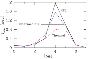
Figure 3: The thermal cooling time scale as a function of $\log\xi$ for all three SEDs, namely, HPL, thermal and intermediate. The density used for the calculations is $n_{\rm H}=10^{14}\rm{cm^{-3}}$ and column density $N_{\rm H}=10^{23}\rm{cm^{-2}}$, for solar metallicity gas.

The stability curves span a wide range of $\xi$ values (Figure 2 dotted black lines cutting across the curves), for most of which all the curves are stable. However, we find that during the HPL state (Figure 2 solid black), hot plasma with $3.55\leq\log\xi\leq 4.20$ is thermodynamically unstable. The ions associated with such gas are therefore unobservable. In contrast, during the intermediate and thermal states, we find that the ionized gas is thermodynamically stable throughout $0\leq\log\xi\leq 6$, and thus a range of ions from low to high Z (atomic number) elements can be detected in these states. All else being equal (e.g. luminosity, density of the gas, and its distance from the central source), detections of ionized winds should be much more common in thermal and intermediate states. Our predictions of the thermodynamic properties of winds in BHB are consistent with the observations that winds are detected in softer, more thermal states and are rarely detected in spectrally hard states (here represented by HPL, e.g. Miller et al. 2008; Neilsen & Lee 2009; Ponti et al. 2012).

In Table 1 we compare the major heating and cooling agents affecting the different BHB state stability curves in an effort to understand what causes the gas ionized by the HPL SED to become unstable at $3.55\leq\log\xi\leq 4.20$. As can be seen, at $\log\xi\sim 4$, Compton heating is far more dominant for the HPL SED ionized gas (79%) than for the thermal SED ionized gas. This affects the temperature, which is higher, due to Comptonization in the former case, and renders the HPL equilibrium curve unstable in the aforementioned $\xi$ range.

Note that for the calculations in Sections 3.1 and 3.2 we have used a gas with constant density $10^{14}\rm{cm^{-3}}$. However, we tested the effect of varying the densities between $10^{5}-10^{14}\rm{cm^{-3}}$ in Section 4.2 and find that the stability curves are insensitive to density variations for $\log\xi\gtrsim 3.0$, leaving the above mentioned results for the range $3.55\leq\log\xi\leq 4.20$ for the HPL state, unchanged.

3.1.1 Thermal time scales

The photoionization calculations performed in this paper are conducted in the static limit. In assessing the relevance of our conclusions for observed ionic differences between BHB states, we calculate the thermal cooling time scale $t_{cool}$ (defined as the time in which the gas looses half of the heat gained by it; Figure 3) of the gas in the static limit. While calculating $t_{cool}$ CLOUDY considers all the heating and cooling processes associated with static gas (some of which are detailed in Table 1). The static gas assumption is reasonable if $t_{cool}$ is less than the adiabatic cooling time scale $t_{ad}$ ($\sim\left[n_{\rm H}kT(a/u+2u/r)\right]^{-1}$, where $a$, $u$ and $r$ are the acceleration, wind velocity, and radius respectively, $k$ being the Boltzmann constant). Calculation of the adiabatic or dynamical time scale is beyond the scope of this paper (but see Begelman et al. 1983; Krolik & London 1983; Chelouche & Netzer 2005; Luketic et al. 2010 for example discussions related to the dynamics of outflowing gas in AGN and X-ray binaries). We do not make any assumptions about the dynamics or the launching mechanisms of the gas. The purpose of this paper is to study the thermodynamics of the photoionized gas, for which we have assumed that the static limit requirements are met.

3.2 Ion Fractions

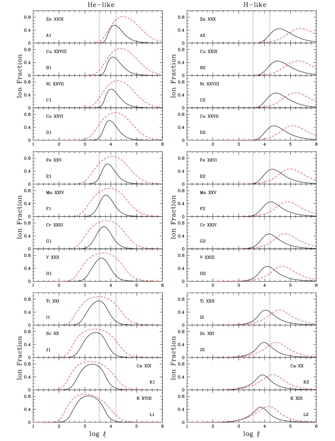
Figure 4: The ion fraction distributions as a function of $\log\xi$ for the HPL (solid black line) and the thermal state (dashed red line) of a BHB. The vertical black dotted lines denote the range $3.55\leq\log\xi\leq 4.20$ over which the absorbing gas is thermodynamically unstable if ionized by the HPL state SED. Note that this unstable $\xi$ range does not apply to the thermal state ion fraction distributions, because the the thermal state stability curves are thermodynamically stable for all values of $\xi$.

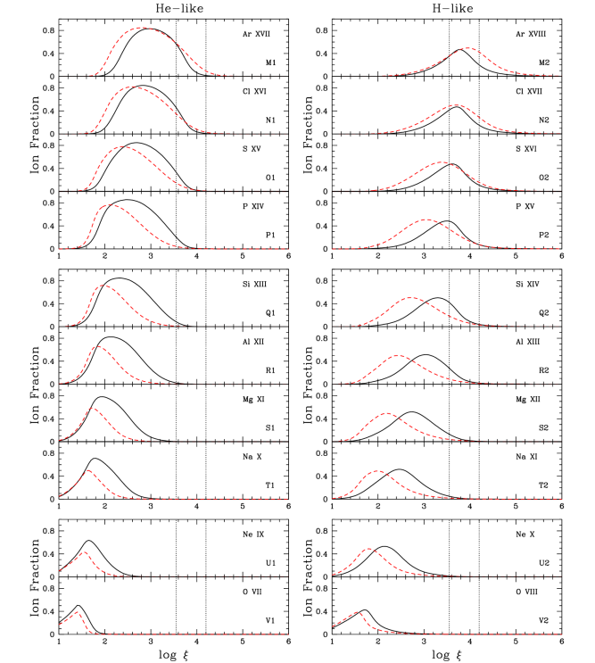
Figure 4: Continued for ions of elements with lower atomic number.

In this section we further investigate the range $3.55\leq\log\xi\leq 4.20$ in terms of ion fractions, to assess thermodynamic instability effects on ion observability. In Figure 4 we plot the $\log\xi$ distribution of the ion fractions of the He-like and H-like ions of all the elements from zinc (atomic no. Z = 30) to oxygen (Z = 8). Vertical lines mark thermodynamically unstable range of $\log\xi$ based on our HPL ionizing SED.

For a given ion if a significant part of the HPL state ion fraction distribution falls within the unstable $3.55\leq\log\xi\leq 4.20$ range, absorption lines of that ion would not be detected. Thus, during the HPL state a number of important He- and H-like species (including Fe xxv) are essentially ‘shrouded’ by the thermodynamically unstable $\xi$ range. Purely from the thermodynamic point of view, these species are not expected to be visible during spectrally hard states. It is notable, however, that the peak ion fraction for Fe xxvi (and higher Z H-like ions) falls outside the unstable $\xi$ range. In other words, if there is a wind in a spectrally hard state with sufficiently high ionization ($\log\xi>4.2$), it could still be detected in Fe xxvi absorption.

The unstable $3.55\leq\log\xi\leq 4.20$ range does not apply to the thermal/intermediate states, since there is no thermal instability. As can be seen from Figures 2 and 4, all ions should be observable from a thermodynamic stability point of view.

These results agree nicely with observational results on the long-term variability of winds. As discussed above, winds are commonly detected through Fe xxv and Fe xxvi absorption during spectrally soft states, and rarely detected during harder states. There are a small number of exceptions, however. For example, in a 2005 Chandra HETGS observation of GROJ1655 during a spectrally hard state, a single Fe xxvi absorption line was seen (Miller et al., 2008; Neilsen & Homan, 2012). Neilsen & Homan (2012) explicitly note the absence of Ar xviii, S xv, and Si xiv in that state. By our calculations, the absence of these ions is not surprising, given that the required $\xi$ for the gas producing these ions would have fallen within the thermodynamically unstable $\xi$ range.

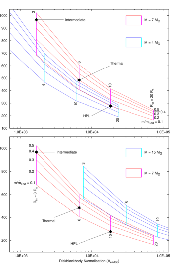
Figure 5: The $T_{max}$ - $A_{ezdbb}$ distribution as a function of the various black hole parameters, $M$, $\dot{m}/\dot{m}_{\rm Edd}$ and $R_{in}/R_{s}$. The fiducial values of the $T_{max}$ and $A_{ezdbb}$ used to generate the SEDs in this paper, are marked as solid black stars on the grid corresponding to $M_{\rm{BH}}=7M_{\odot}$ (red-and-magenta). In the top panel we compare the standard $M_{\rm{BH}}=7M_{\odot}$ distribution to that of a lower $M_{\rm{BH}}=4M_{\odot}$ black hole, and in the bottom panel with that of an higher $M_{\rm{BH}}=15M_{\odot}$ one.

4 Discussion

The fiducial SEDs discussed in Section 2 and shown in Figure 1, although generic representations of the respective states, were generated using certain SED parameters. In this section we investigate the effects of varying SED parameters - $M,\,\,\dot{m}\,\,\rm{and}\,\,R_{in}$ (Section 4.1.1), $f_{d}$ and $\Gamma$ (Section 4.1.2) and powerlaw break $E_{b}$ (Section 4.1.3) on thermodynamic stability results. We find that physically and observationally reasonable variations of these parameters do not alter the conclusions of our thermodynamic calculations (Section 3). The same is true for variations in the wind density (Section 4.2)

4.1 Variations in the SED parameters

4.1.1 Variations in $M,\,\,\dot{m}\,\,\rm{and}\,\,R_{in}$

A plausible range of black hole masses lie between $M\sim 4M_{\odot}$ (e.g. XTE J1650–500 Orosz et al. 2004) and $M\sim 15M_{\odot}$ (e.g see Greiner et al. 2001 for GRS 1915-105, Orosz et al. 2007 for M 33 X-7 and Orosz et al. 2011 for Cygnus X-1). As discussed in Section 2, we choose a black hole of mass $M_{\rm{BH}}=7M_{\odot}$ (based on GROJ1655) to represent a generic BHB. We further chose particular sets of $\dot{m}/\dot{m}_{\rm Edd}$ and $R_{in}/R_{s}$ that correspond to values of $T_{max}$ and $A_{ezdbb}$ typically observed in outbursts of BHBs.

Given the relationship between temperature, disk radius, accretion rate, and black hole mass (Equation 1), how much are the SEDs affected by variations in $M_{\rm{BH}}$? In Figure 5, we have compared the relationship between $T_{max}$ and $A_{ezdbb}$ for a $7M_{\odot}$ black hole to that of a $4M_{\odot}$ and a $15M_{\odot}$ black hole. The fiducial values for our three SEDs are marked as solid black stars. The top panel of Figure 5 shows that for reasonable accretion rates and inner disk radii, our thermal/HPL SEDs could apply to a $4M_{\odot}$ black hole; the intermediate SED requires higher accretion rates ($\dot{m}>0.5\dot{m}_{\rm Edd}$), but not unheard of in BHBs. The $15M_{\odot}$ black hole can also match the fiducial values of $T_{max}$ with reasonable values of $\dot{m}/\dot{m}_{\rm Edd}$ and $R_{in}/R_{s}$, although the implied disk normalizations are a factor of $\sim 5$ larger. Thus we believe that our SEDs can be considered broadly representative of BHBs at a range of masses, accretion rates, and disk radii.

4.1.2 Variations in disk fraction $f_{disk}$ and $\Gamma$

As discussed, we have followed the scheme of Remillard & McClintock (2006) to pick reasonable combinations for accretion disk and power law components (see Section 2). Since our stability curves are dependent on overall spectral shape, it is imperative to test if our results (derived from the stability curves) are robust to variations in $f_{d}$ and $\Gamma$

Remillard & McClintock (2006) define the thermal state as having $f_{d}>0.75$. Keeping our $\Gamma$ constant at 2.5, we calculated new stability curves for $f_{d}(0.7,0.8,0.9)$, and found no changes in the thermodynamic stability of the gas. Since Remillard & McClintock (2006) do not state a particular range for $\Gamma$, we vary $1.4\leq\Gamma\leq 3.0$ (in steps of 0.2) keeping $f_{d}=0.8$ constant. For $\Gamma<2.0$ the curve becomes unstable in the range $3.84\leq\log\xi\leq 4.24$. However, a literature survey reveals no instances of $\Gamma<2$ in the thermal state. Hence we conclude that during the thermal state, winds should be thermodynamically stable for all values of $\xi$.

In addition Remillard & McClintock (2006) define the spectrally hard state (which we call the HPL state) as having $f_{d}<0.2$ and $1.4\leq\Gamma\leq 2.1$. Varying $f_{d}(0.1,0.2)$ while keeping $\Gamma=1.8$ constant and then varying $1.4\leq\Gamma\leq 2.2$ (in steps of 0.2) while keeping $f_{d}=0.2$ constant we find that the curve retains the unstable $\xi$ range discussed in Section 3.

Thus the qualitative results presented in Section 3 hold for the entire range of the parameters of X-ray emission defined by Remillard & McClintock (2006) for the BHB states.

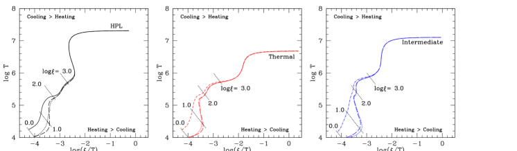
Figure 6: The effects of density variation on the stability curves are shown for the three BHB states (HPL in the left panel, thermal in the middle panel and intermediate in the right panel). Other than the fiducial density value of $n_{\rm H}=10^{14}\rm{cm^{-3}}$ (for which we maintain the same line styles as in Figure 2 - dashed for thermal, dashed-and-dotted for intermediate and solid for HPL), in each panel we consider two additional densities $n_{\rm H}=10^{10}\rm{cm^{-3}}$ (long-dashed) and $n_{\rm H}=10^{6}\rm{cm^{-3}}$ (dotted). For each SED the stability curves are identical for $\log\xi\geq 3.0$, showing that density does not affect the heating and cooling at these ionization parameters. However, for lower $\xi$, the constant $\xi$, diagonal dotted black line segments are maintained to show the range of ionization parameter where density effects are important.

4.1.3 Variations in the powerlaw break energy $E_{b}$

For all the SEDs discussed in the previous sections, the parameters for the exponential cut-off in the powerlaw (Equation 4) were chosen such that the powerlaw had a break at $E_{b}\sim 100\,{\rm keV}$. Observations of spectrally hard (HPL) states of BHBs show powerlaw breaks at $E_{b}\sim 100\,{\rm keV}$, but for thermal states the break is usually observed at much lower energies $E_{b}\sim 20-30\,{\rm keV}$. It is believed that this has to do with the presence or absence of jets (and associated particle acceleration processes) in these states. Regardless of the origin of changes in the break energy, though, the effect on thermodynamic conditions is worth investigating, so we calculated new stability curves for $E_{b}=20,40,\,\,\rm{and}\,\,80\,{\rm keV}$, both for the thermal and HPL states.

Based on our analysis, the stability curves are insensitive to the variation in $E_{b}$ for $\log{\rm T}<5.7$ (K) or $\log\xi<3.0$. At higher temperatures, the stability curves become more smooth and the plasma actually becomes more stable as the break energy decreases from 100 keV to 20 keV. This does not affect our conclusions for the thermal state, since the plasma was already stable at all $\xi$.

However, one consequence of variations in $E_{b}$ is that during the HPL state, the aforementioned range $3.55\leq\log\xi\leq 4.20$ becomes thermodynamically stable (see Section 3) as $E_{b}$ is decreased to 20 keV. The theoretical reason for this effect is easy to understand, where one recalls the discussion on heating and cooling agents in Section 3.1. According to Table 1, at high ionization parameters ($\log\xi\sim 4.0)$, the temperature of the gas ionized by HPL SED is determined by Compton heating (79% contribution) when $E_{b}=100\,{\rm keV}$. However, if $E_{b}\sim 20\,{\rm keV}$, then there is a significant decrease in the number of high energy photons thus reducing the extent of Comptonization (Comptonization contributes only 49% to heating) . Hence the temperature of the gas decreases resulting in a thermodynamically stable distribution of temperature and pressure. Although theoretically noteworthy, this is not a relevant result because the jet dominated HPL state is not likely to have such low break in the powerlaw. Thus, variation in the powerlaw break $E_{b}$ also does not affect the results in Section 3, unless there are reasons to consider that the HPL state continuum has a low powerlaw break at $\sim 20\,{\rm keV}$.

4.2 Variations in wind density

We vary the particle density of the absorbing gas between $n_{\rm H}=10^{5}-10^{14}\rm{cm^{-3}}$ and generate stability curves (Figure 6) for the HPL state (left panel), the thermal state (middle panel) and the intermediate state (right panel) SEDS, to determine if the results presented in Section 3 are susceptible to density effects. As can be seen from the figure, density variations do not have any effect on the stability curves for $\log\xi\gtrsim 3.0$ and the effect is small until $\log\xi<2.0$. For lower $\log\xi$ the stability curves are seen to be thermodynamically unstable if the wind has density $n_{\rm H}\lesssim 10^{10}\rm{cm^{-3}}$. Because the vast majority of plasma in BHBs can be described by ionization parameters $\log\xi\sim 4$ (with the exception of GX 339-4, $\xi\sim 70$; Miller et al. 2004), our conclusions for the thermodynamic stability (or lack of it) of winds are not affected by gas density variations.

Even though we primarily see high $\xi(\log\xi\gtrsim 4)$ gas in BHBs, we still consider density effects at low $\xi(\log\xi\lesssim 2.0)$ to improve theoretical understanding. Figure 6 shows that the greatest difference in the gas temperature occurs at $\log\xi\sim 1.0$ in comparing plasma with $n_{\rm H}\leq 10^{10}\rm{cm^{-3}}$ to one with $n_{\rm H}=10^{14}\rm{cm^{-3}}$. Referring back to Table 1 we find the detailed heating and cooling agents corresponding to the different stability curves. Specifically, comparing the results for $\log\xi=1.0$ in Table 1, the heating and cooling agents and their fractional contributions are similar for $n_{\rm H}=10^{6}\,\,\rm{and}\,\,10^{10}\rm{cm^{-3}}$ but differ from that of $n_{\rm H}=10^{14}\rm{cm^{-3}}$. An explanation is that - line cooling is dominant for $n_{\rm H}\leq 10^{10}\rm{cm^{-3}}$, whereas continuum processes like free-free cooling, recombination cooling and radiation through emission of iso-sequences of Hydrogen and Helium are dominant cooling mechanisms for $n_{\rm H}=10^{14}\rm{cm^{-3}}$ resulting in higher temperatures in the later case.

5 Conclusions

We have constructed fiducial SEDs for the thermal, intermediate and HPL states of the BHBs, following the prescription of Remillard & McClintock (2006) for a typical $7M_{\odot}$ black hole, based on GROJ1655. Using these SEDs we generated thermodynamic stability curves for each state to arrive at the following conclusions:

1. In the thermal and intermediate state all phases of the wind is thermodynamically stable (§Section 3.1). However, the ionization parameter range $3.55\leq\log\xi\leq 4.20$ is thermodynamically unstable for winds in the HPL state. We found that a large number of the He-like ions (21 $<$ Z $<$ 30, Ti through Cu) and H-like ions (15 $<$ Z $<$ 25, S through Mn) have peak ion fractions in the unstable ionization parameter range for the HPL state, making the lines from these ions potentially unobservable (§Section 3.2).

2. Our findings are well corroborated in the observational literature, since there appears to be a gradient in wind properties with BHB state. In accord with their thermodynamic stability (and lack of it for spectrally harder HPL states), winds are predominantly observed in intermediate and soft/thermal states and have weak or absent lines from Fe xxv and low-Z elements in the HPL states (Lee et al., 2002; Miller et al., 2008; Neilsen & Lee, 2009; Blum et al., 2010; Ponti et al., 2012; Neilsen & Homan, 2012). In the HPL state, while the ions with peak ion fractions in the unstable $\xi$ range may be unobservable, Fe xxvi may remain detectable at high ionization parameters ($\log\xi>4.2$) in such states (based on our calculations in Section 3.2 and consistent with observations noted by Neilsen & Homan 2012).

3. In general, a range of ionizations are thermodynamically stable (except for $3.55\leq\log\xi\leq 4.20$ for HPL state) in all the states we have studied here. Yet the observed absorbers are usually consistent with a single high ionization parameter. This may indicate a genuine absence of plasma at lower ionization. On the other hand, for many other sources intervening cold absorption from the source or the ISM may be the reason.

4. There have been suggestions for magnetically driven winds in e.g GROJ1655 (Miller et al., 2008; Neilsen & Homan, 2012). The pressure term in the temperature - pressure distributions (stability curves) considered in this paper deals with only the thermodynamic gas pressure on the photoionised medium (through $\xi/T$). Magnetic pressure in not included in such calculations. It would be interesting to incorporate the magnetic pressure term, which would change the stability conditions from what we have shown in this paper. Given a reasonable description of the magnetic field in the photoionized medium, codes like CLOUDY are capable of such calculations. In our future publications we shall formulate this phase space as a diagnostic tool for photoionized gas which are under the influence of strong magnetic fields.

References

- Allende Prieto et al. (2001) Allende Prieto, C., Lambert, D.L., & Asplund, M., 2001, ApJ, 556, L63
- Allende Prieto et al. (2002) Allende Prieto, C., Lambert, D.L., & Asplund, M., 2002, ApJ, 573, L137
- Arnaud (1996) Arnaud, K. A. 1996, ASPC, 101, 17
- Begelman et al. (1983) Begelman, M.C.; McKee, C.F. & Shields G.A. 1983, ApJ, 271,70
- Blum et al. (2010) Blum, J. L.; Miller, J. M.; Cackett, E.; Yamaoka, K.; Takahashi, H.; Raymond, J.; Reynolds, C. S.; Fabian, A. C. 2010, ApJ, 713, 1244
- Brandt & Schulz (2000) Brandt, W. N.; Schulz, N. S. 2000, ApJ, 544L, 123
- Chakravorty et al. (2008) Chakravorty, S., Kembhavi, A.K., Elvis, M., Ferland, G. & Badnell, N.R., 2008, MNRAS, 384L, 24
- Chakravorty et al. (2009) Chakravorty, S., Kembhavi, A.K., Elvis, M. & Ferland, G., 2009, MNRAS, 393, 83
- Chelouche & Netzer (2005) Chelouche, D. & Netzer, H. 2005, ApJ, 625, 95
- Canizares et al. (2005) Canizares, C. et al. 2005, PASP, 117, 1144
- Chakravorty et al. (2012) Chakravorty, S., Misra, R., Elvis, M., Kembhavi, A.K., & Ferland, G., 2009, MNRAS, 393, 83
- Ferland et al. (1998) Ferland, G. J.; Korista, K. T.; Verner, D. A.; Ferguson, J. W.; Kingdon, J. B.; Verner, E. M. 1998, PASP, 110, 761
- Frank, King & Raine (2002) Frank, J., King, A., & Raine, D. 2002, Accretion Power in Astrophysics (3rd ed.; Cambridge: Cambridge Univ. Press)
- Greiner et al. (2001) Greiner, J.; Cuby, J. G.; McCaughrean, M. J. 2001, Nature, 414, 522
- Grevesse & Sauval (1998) Grevesse, N., & Sauval, A.J., 1998, Space Science Review, 85, 161
- Hanke et al. (2009) Hanke, M.; Wilms, J.; Nowak, M. A.; Pottschmidt, K.; Schulz, N. S.; Lee, J. C. 2009, ApJ, 690, 330
- Hess et al. (1997) Hess, C.J.; Kahn, S.M.; Paerels, F.B.S., 1997, ApJ, 478, 94
- Holweger (2001) Holweger, H., 2001, Joint SOHO/ACE workshop “Solar and Galactic Composition”. Edited by Robert F. Wimmer-Schweingruber. Publisher: American Institute of Physics Conference proceedings, 598, 23
- Jimenez-Garate et al. (2002) Jimenez-Garate, M. A., Raymond, J. C., & Liedahl, D. A. 2002, ApJ, 581, 1297
- Kallman et al. (2009) Kallman, T. R.; Bautista, M. A.; Goriely, S.; Mendoza, C.; Miller, J. M.; Palmeri, P.; Quinet, P.; Raymond, J. 2009, ApJ, 701, 865
- King et al. (2012) King, A. L. et al. 2012, ApJ, 746L, 20
- Krolik et al. (1981) Krolik, J. H., McKee, C. F., & Tarter, C. B. 1981, ApJ, 249, 422
- Krolik & London (1983) Krolik, J. H., London, R.A. 1983, ApJ, 267,18
- Lee et al. (2002) Lee, J. C. and Reynolds, C. S. and Remillard, R. and Schulz, N. S. and Blackman, E. G. and Fabian, A. C. 2002, ApJ, 567, 1102
- Lee et al. (2013) Lee, J. C et al. 2013, In Press, arXiv1301.3148
- Luketic et al. (2010) Luketic, S., Proga, D., Kallman, T. R., Raymond, J.C., Miller, J.M. 2010, ApJ, 719, 515
- Miller et al. (2004) Miller et al. 2004, ApJ, 601, 450
- Miller et al. (2006) Miller, J. M.; Raymond, J.; Homan, J.; Fabian, A. C.; Steeghs, D.; Wijnands, R.; Rupen, M.; Charles, P.; van der Klis, M.; Lewin, W. H. G. 2006, ApJ, 646, 394
- Miller et al. (2008) Miller, J. M. and Raymond, J and Reynolds, C. S. and Fabian, A. C. and Kallman, T. R. and Homan, J. 2008, ApJ, 680, 1359
- Miller et al. (2011) Miller, Jon M.; Maitra, Dipankar; Cackett, Edward M.; Bhattacharyya, Sudip; Strohmayer, Tod E. 2011, ApJ, 731L, 7
- Miller et al. (2012) Miller et al. 2012, ApJ, 759L, 6
- Neilsen & Lee (2009) Neilsen, J; Lee, J. C. 2009, Natur, 458, 481
- Neilsen et al. (2009) Neilsen, J; Lee, J. C.; Nowak, M. A.; Dennerl, K.; Vrtilek, S. D. 2009, ApJ, 696, 182
- Neilsen et al. (2011) Neilsen, J.; Remillard, R. A.; Lee, J. C. 2011, ApJ, 737, 69
- Neilsen & Homan (2012) Neilsen, J.; Homan, J. arXiv1202.6053
- Neilsen et al. (2012) Neilsen, J.; Petschek, A. J.; Lee, J. C. 2012, MNRAS, 421, 502
- Orosz et al. (1997) Orosz, J., & Baily, C. D. 1997, ApJ, 477, 876
- Orosz et al. (2004) Orosz, J.; McClintock, J. E.; Remillard, R. A.; Corbel, S. 2004, ApJ, 616, 376
- Orosz et al. (2007) Orosz, J.et al. 2007, Nature, 449, 872O,
- Orosz et al. (2011) Orosz, J.; McClintock, J. E.; Aufdenberg, J. P.; Remillard, R. A.; Reid, M. J.; Narayan, R.; Gou, L. 2011, ApJ, 742, 84
- Peterson (1997) Peterson, B. M. 1997, An Introduction to Active Galactic Nuclei. Cambridge Univ. Press, Cambridge.
- Ponti et al. (2012) 2012, MNRAS.tmpL, 417; arXiv:1201.4172
- Proga et.al (1998) Proga, D.; Stone, J. M.; Drew, J. E. 1998, MNRAS, 295, 595
- Proga (2003) Proga, D. 2003, ApJ, 585, 406