Spin-1/2 $J_{1}$–$J_{2}$ Heisenberg model on a cross-striped square lattice

Abstract

Using the coupled cluster method (CCM) we study the full (zero-temperature) ground-state (GS) phase diagram of a spin-half ($s=\frac{1}{2}$) $J_{1}$–$J_{2}$ Heisenberg model on a cross-striped square lattice. Each site of the square lattice has 4 nearest-neighbor exchange bonds of strength $J_{1}$ and 2 next-nearest-neighbor (diagonal) bonds of strength $J_{2}$. The $J_{2}$ bonds are arranged so that the basic square plaquettes in alternating columns have either both or no $J_{2}$ bonds included. The classical ($s\rightarrow\infty$) version of the model has 4 collinear phases when $J_{1}$ and $J_{2}$ can take either sign. Three phases are antiferromagnetic (AFM), showing so-called Néel, double Néel and double columnar striped order respectively, while the fourth is ferromagnetic. For the quantum $s=\frac{1}{2}$ model we use the 3 classical AFM phases as CCM reference states, on top of which the multispin-flip configurations arising from quantum fluctuations are incorporated in a systematic truncation hierarchy. Calculations of the corresponding GS energy, magnetic order parameter and the susceptibilities of the states to various forms of valence-bond crystalline (VBC) order are thus carried out numerically to high orders of approximation and then extrapolated to the (exact) physical limit. We find that the $s=\frac{1}{2}$ model has 5 phases, which correspond to the four classical phases plus a new quantum phase with plaquette VBC order. The positions of the 5 quantum critical points are determined with high accuracy. While all 4 phase transitions in the classical model are first order, we find strong evidence that 3 of the 5 quantum phase transitions in the $s=\frac{1}{2}$ model are of continuous deconfined type.

I INTRODUCTION

Magnetic models involving quantum spin systems on regular two-dimensional (2D) lattices have been at the center of both theoretical and experimental condensed matter research in recent times (see, e.g., Refs. 2D_magnetism_1, ; 2D_magnetism_2, ). Even when such systems are described in terms of seemingly very simple Hamiltonians they can often display a bewildering variety of ground-state (GS) phases with different types of ordering, even at zero temperature ($T=0$). The phases of the quantum systems (with spins of a finite nonzero value of the spin quantum number, $s$), and the transitions between them as some internal control parameter is varied across the corresponding quantum critical points (QCPs), often differ widely from those of their classical ($s\rightarrow\infty$) counterparts. Such control parameters usually provide a measure of the degree of dynamic frustration between competing interactions in the system. Since it is widely believed that many of the properties of a large variety of interesting strongly-correlated quantum many-body systems can be understood in terms of the competition between GS phases with qualitatively different properties, particular interest has focussed on the associated quantum phase transitions and the behavior of the system near such QCPs (see, e.g., Refs. Sachdev:1999, ; Sentil:2004, ; Sachdev:2011, ).

The often subtle interplay between frustration and quantum fluctuations can lead to quantum spin-lattice models exhibiting $T=0$ GS phase diagrams that are very different from their classical counterparts. Since quantum effects tend to diminish as the spin quantum number increases, spin-1/2 models have a special role to play. Whereas many phase transitions in classical systems are often of first-order type, where the transition between the two phases involves sudden jumps in many of the physical properties, quantum fluctuations can even act to turn such a first-order classical transition into a (continuous) second-order one. Precisely at or very near such a second-order QCP the GS phase has very special properties. The GS wave function becomes a complex superposition of an exponentially large set of multispin configurations that fluctuate at all length scales, and hence it exhibits long-range entanglement phenomena. Such GS wave functions are very different from those of the quasiclassical states that often lie on one or other (or both) sides of the QCP in the GS phase diagram, and whose wave functions can be described in simple terms as a product state for all the spins. Of course, quantum fluctuations still produce a mixture of other “wrong” multispin configurations on top of such a simple product state, but far from the QCP they do not totally destroy the classical order present in the simple quasiclassical state.

The traditional Landau-Ginzburg-Wilson (LGW)Landau:1999 ; Wilson:1974 description of quantum second-order transitions and their associated critical singularities and quantum critical phenomena has been remarkably successful in describing many quantum phase transitions. However, it has become clear in recent years that there are other continuous transitions that do not fit the LGW paradigm for critical phenomena in which the critical singularities are associated with the fluctuations of some appropriate order parameter that captures the essential difference between the two phases on either side of the transition. In particular, it has been shownSentil:2004 how subtle quantum interference effects can invalidate the LGW paradigm of QCPs separating phases characterized by such standard confining order parameters, by the appearance of an emergent gauge field and consequent deconfined degrees of freedom which are associated with the fractionalization of the appropriate order parameters. Thus, in this alternate deconfined scenario an emergent gauge field mediates the interactions between the associated emergent particles that carry fractions of the quantum numbers corresponding to the underlying degrees of freedom. Such fractional particles are confined at low energies so that they do not appear sufficiently far away on either side of the QCP, but they emerge naturally (and hence deconfine) just at the QCP. Such deconfined second-order phase transitions can occur between states that break different symmetries, a scenario which is not allowed in the standard LGW description.

Since quantum-critical states themselves are so inherently complex they have largely been studied using either techniques from quantum field theory or large-scale numerical simulations, usually of the quantum Monte Carlo (QMC) kind. It is clear that near QCPs, where the effects of quantum fluctuations, and hence the complexity of the wave functions, increase the closer one approaches them, very accurate quantum many-body techniques are needed. One such method is the coupled cluster method (CCM),Bi:1991 ; Bishop:1998 ; Fa:2004 which has very successfully been applied to a wide variety of frustrated quantum spin-lattice models (see, e.g., Refs. Fa:2004, ; Ze:1998, ; Bishop:1998_J1J2mod, ; Kr:2000, ; Bishop:2000, ; Fa:2001, ; Darradi:2005, ; Schm:2006, ; Bi:2008_PRB_J1xxzJ2xxz, ; Bi:2008_JPCM, ; darradi08, ; Bi:2009_SqTriangle, ; Darradi:2009_J1J2_XXZmod, ; richter10:J1J2mod_FM, ; Bishop:2010_UJack, ; Bishop:2010_KagomeSq, ; Reuther:2011_J1J2J3mod, ; DJJF:2011_honeycomb, ; Gotze:2011, ; Bishop:2012_honey_phase, ; Bishop:2012_checkerboard, ; Li:2012_honey_full, ; Bishop:2012_honeyJ1-J2, ; Li:2012_anisotropic_kagomeSq, ; RFB:2013_hcomb_SDVBC, ; Li:2013_chevron, ), yielding a good description of their $T=0$ GS phase diagrams and accurate numerical values for their QCPs, even ones involving deconfined transitions (see, e.g., Refs. DJJF:2011_honeycomb, ; Bishop:2012_honeyJ1-J2, ; Li:2012_honey_full, ; RFB:2013_hcomb_SDVBC, ).

The CCM has been found to yield accurate descriptions of quantum magnets with different types of both quasiclassical magnetic order and quantum paramagnetic order, including various types of valence-bond crystalline (VBC) order. These include the prototypical $J_{1}$–$J_{2}$ model on the square lattice, Bishop:1998_J1J2mod ; darradi08 which contains nearest-neighbor (NN) Heisenberg interactions with exchange coupling strength $J_{1}$ and corresponding next-nearest-neighbor (NNN) (i.e., diagonal) bonds of strength $J_{2}$, as well as models that generalize it by introducing both spatial lattice anisotropyBi:2008_JPCM and spin anisotropy.Bi:2008_PRB_J1xxzJ2xxz ; Darradi:2009_J1J2_XXZmod Of particular interest for present purposes, they also include models in the so-called half-depleted $J_{1}$–$J_{2}$ class, in the sense that they are obtained from the full $J_{1}$–$J_{2}$ model on the square lattice by removing half of the $J_{2}$ bonds in different arrangements. Examples include: (a) the ($J_{1}$–$J_{2}^{\prime}$ or) interpolating square-triangle model,Bi:2009_SqTriangle (b) the so-called Union Jack model,Bishop:2010_UJack (c) the anisotropic planar pyrochlore (APP) model (also known as the crossed chain model) that comprises a $J_{1}$–$J_{2}$ model on the checkerboard lattice,Bishop:2012_checkerboard and (d) an analogous $J_{1}$–$J_{2}$ model on a chevron-square lattice.Li:2013_chevron

This half-depleted $J_{1}$–$J_{2}$ class of models on the square lattice exhibits a wide variety of GS phase diagrams and QCPs, all of which pose serious theoretical challenges, but which serve to improve our understanding of quantum critical phenomena. In the current paper we consider another member of this class, namely the spin-1/2 $J_{1}$–$J_{2}$ Heisenberg model on a cross-striped square lattice, and we find that it too has a rich $T=0$ GS phase diagram that includes many of the features discussed above.

As a motivation for this study we note that while it is true that there are many different ways that a Heisenberg antiferromagnet might be frustrated in principle, the $J_{1}$–$J_{2}$ model and its depleted counterparts occupy a central role. Of the half-depleted class described above there are two principal sub-classes. The first is where each square plaquette (formed from four NN $J_{1}$ bonds) contains one $J_{2}$ bond. The three main members of this sub-class have been well studied previously. They comprise (a) the interpolating square-triangle lattice model,Bi:2009_SqTriangle (b) the Union Jack lattice model,Bishop:2010_UJack and (c) the chevron-decorated square lattice model.Li:2013_chevron These have the respective features that the arrangements of the remaining diagonal NNN $J_{2}$ bonds are such that in case (a) the $J_{2}$ bonds are all parallel, while in case (b) the orientations of the $J_{2}$ bonds alternate along both rows and columns, and in case (c) the orientations of the $J_{2}$ bonds is the same along one square-lattice axis direction (say, rows) but alternates along the perpendicular direction (say, columns). The second principal sub-class is where half the basic square plaquettes have both $J_{2}$ bonds (namely, the filled squares) while the remainder have neither (namely, the empty squares). There are clearly now two main members of this sub-class, namely (i) where the empty and filled squares alternate along both rows and columns (which is precisely the anisotropic planar pyrochlore model or checkerboard lattice modelBishop:2012_checkerboard that has received much previous attention), and (ii) where alternating columns, say, comprise filled squares and empty squares (which is precisely the present cross-striped square lattice model). From among all members of the above two sub-classes only the latter model seems not to have been studied before now.

                   

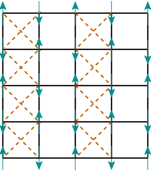
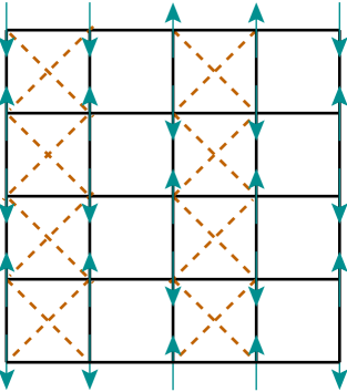
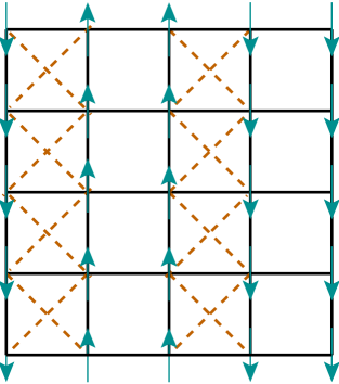
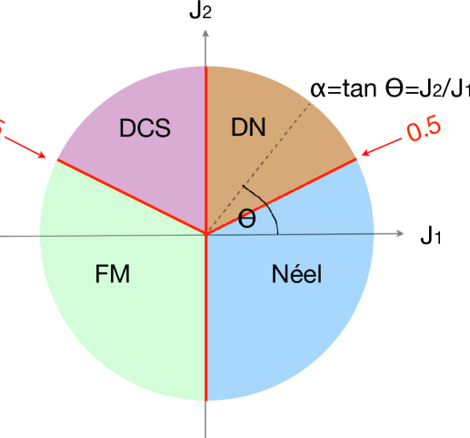
Figure 1: (Color online) The $J_{1}$–$J_{2}$ Heisenberg model on a cross-striped square lattice. The solid (black) lines are $J_{1}$ bonds and the dashed (brown) lines are $J_{2}$ bonds. The (cyan) arrows represent the relative spin directions in: (a) the Néel state, (b) the double Néel (DN) state, and (c) the double columnar striped (DCS) state. (d) The classical phase diagram of the model.

As additional motivation for this study we note that the successful continual syntheses of new quasi-2D magnetic materials, and the experimental observations of their properties, provides an ongoing challenge for the theorist. While we are unaware of any experimental realization of the current cross-striped square-lattice model, several already exist for other members of the depleted $J_{1}$–$J_{2}$ class. For example, for the related interpolating square-triangle model, Bi:2009_SqTriangle the magnetic material Cs₂CuCl₄ provides a good experimental realization. We suspect that similar candidates will soon emerge as realizations of the current model. Perhaps even more exciting, however, is the prospect of being able to realize spin-lattice models with ultracold atoms trapped in appropriate optical lattices,Struck:2011 with the subsequent ability to tune the strengths of the competing NN $J_{1}$ bonds and NNN $J_{2}$ bonds, and hence to drive the system from one GS phase to another, thereby exploring the QCPs experimentally.

We now describe the model in detail in Sec. II, before outlining the main features of the CCM in Sec. III. Our results are presented and discussed in Sec. IV, and we summarize and conclude in Sec. V where the full GS phase diagram for the model is presented.

II THE MODEL

The model considered here is the so-called $J_{1}$–$J_{2}$ Heisenberg model on the cross-striped square lattice. Its Hamiltonian is written as

$$H=J_{1}\sum_{\langle i,j\rangle}\mathbf{s}_{i}\cdot\mathbf{s}_{j}+J_{2}\sum_{\langle\langle i,k\rangle\rangle^{\prime}}\mathbf{s}_{i}\cdot\mathbf{s}_{k}\,,$$ (1)

where the operators $\mathbf{s}_{i}\equiv(s^{x}_{i},s^{y}_{i},s^{z}_{i}$) are the usual quantum spin operators on lattice site $i$, with ${\bf s}^{2}_{i}=s(s+1)$. Here we concern ourselves only with the extreme quantum case where all lattice sites are occupied by a spin with spin quantum number $s=\frac{1}{2}$. On the underlying square lattice the sum over $\langle i,j\rangle$ in Eq. (1) runs over all distinct NN bonds (each of which has the same exchange coupling strength $J_{1}$), whereas the corresponding sum over $\langle\langle i,k\rangle\rangle^{\prime}$ runs over only half of the distinct NNN (diagonal) bonds (each of which has the same exchange coupling strength $J_{2}$). In the latter sum half of the basic square plaquettes, the so-called filled squares, have both diagonal ($J_{2}$) bonds included, while the remainder, the empty squares, have neither diagonal bond included. The pattern of the filled and empty squares, as shown in Fig. 1, is such that along one of the basic square-lattice directions (say, along rows) filled and empty squares alternate, while along the perpendicular direction (say, along columns) the squares are either all empty or all filled. Thus, the $J_{1}$–$J_{2}$ model on the cross-striped square lattice differs from the corresponding APP model on the checkerboard lattice simply by the pattern of filled and empty squares. Both models contain equal numbers of filled and empty squares, but in the APP model the empty and filled squares alternate along both rows and columns. The primitive unit cell on the cross-striped square lattice, as shown in Fig. 1, thus has size $2\times 1$. In both sums in Eq. (1) each bond is counted only once.

We are interested here in the full $T=0$ GS phase diagram of the model, and hence in each of the cases where both types of bonds are (independently) either ferromagnetic (FM) or antiferromagnetic (AFM) in nature. Since the overall energy scale is irrelevant for the phase diagram, once we have specified the sign of either $J_{1}$ or $J_{2}$, the model is completely specified by the ratio $\alpha\equiv J_{2}/J_{1}$. Let us first consider the simpler case when $J_{2}<0$ (and hence the NNN bond is FM in character). In this case the (independent) one-dimensional (1D) zigzag chains joined by $J_{2}$ bonds prefer to have FM order, and for either sign of $J_{1}$ the system is unfrustrated since the ordering directions of different chains is not fixed by the sign of $J_{2}$ alone. Thus, if $J_{1}<0$ the classical ($s\rightarrow\infty$) system will take overall FM ordering, while for $J_{1}>0$ the system will take Néel AFM ordering. Conversely, in the more complicated case when $J_{2}>0$, such that the 1D zigzag chains connected by $J_{2}$ bonds prefer Néel AFM order along them, the $J_{1}$ bonds will act to frustrate this order for either sign of $J_{1}$.

In order to place our later work for the $s=\frac{1}{2}$ model in context, let us first consider its classical ($s\rightarrow\infty$) counterpart. It is straightforward to show that the classical $J_{1}$–$J_{2}$ model on the cross-striped square lattice has four GS phases, separated by four first-order phase transitions, all as shown in Fig. 1(d). Firstly, the Néel AFM phase, which is shown in Fig. 1(a), and which forms the stable GS phase for $J_{1}>0$ and $J_{2}=0$, persists as the frustration is increased (i.e., with $J_{2}>0$) until a first critical point $\alpha^{{\rm cl}}_{1}\equiv\frac{1}{2}$, where it undergoes a first-order phase transition to another collinear AFM phase, the so-called double Néel (DN) phase, shown in Fig. 1(b). This state has AFM Néel ordering along the square-lattice axis direction parallel to the cross-stripes of filled squares (i.e., along columns in Fig. 1), but with spins alternating in a pairwise fashion in the perpendicular direction (i.e., along rows in Fig. 1), such that on filled (empty) squares NN spins are parallel (antiparallel) in the row direction. This DN state itself now persists as the frustration parameter $\alpha$ is further increased. If we define $\alpha\equiv\tan\theta$, such that the full phase diagram is specified by $\theta$ in the range $0\leq\theta<2\pi$, then the DN state is the stable GS phase in the range $\theta^{{\rm cl}}_{1}<\theta<\theta^{{\rm cl}}_{2}$, with $\theta^{{\rm cl}}_{1}=\tan^{-1}(\frac{1}{2})$ and $\theta^{{\rm cl}}_{2}=\frac{1}{2}\pi$. At the second critical point, $\theta^{{\rm cl}}_{2}$, as $J_{1}$ now is allowed to become negative (i.e., so that $\theta$ increases beyond $\frac{1}{2}\pi$), the DN phase gives way to a third collinear AFM phase, the so-called double columnar striped (DCS) phase shown in Fig. 1(c). Both the DN and DCS phases have Néel ordering along the independent 1D zigzag chains joined by $J_{2}$ bonds. Like the DN state, the DCS state also has spins alternating in a pairwise fashion in the square-lattice axis direction perpendicular to the cross-stripes of filled square (i.e., along rows in Fig. 1), but now such that on empty (filled) squares NN spins are parallel (antiparallel) in the row direction. On the other hand, in the perpendicular direction (i.e., along columns in Fig. 1), the spins in the DCS state form FM chains, with the orientation of the spins now alternating in a pairwise fashion, as shown in Fig. 1(c). This DCS state itself forms the stable GS phase over the range $\theta^{{\rm cl}}_{2}<\theta<\theta^{{\rm cl}}_{3}$, with $\theta^{{\rm cl}}_{3}=\tan^{-1}(-\frac{1}{2})$. Finally, at $\alpha^{{\rm cl}}_{3}=-\frac{1}{2}$ the DN phase gives way to the FM phase, which itself persists over the range $\theta^{{\rm cl}}_{3}<\theta<\theta^{{\rm cl}}_{4}$, with $\theta^{{\rm cl}}_{4}=\frac{3}{2}\pi$. Finally, at the fourth critical point, $\alpha^{{\rm cl}}_{4}$, there is a first-order transition between the FM and Néel AFM phases.

Compared to the classical ($s\rightarrow\infty$) version of the $J_{1}$–$J_{2}$ model on the cross-striped square lattice, the GS phase of the $s=\frac{1}{2}$ model is really only well established at a few special values of the parameter $\theta$. Firstly, for the case $\theta=0$, corresponding to the isotropic square-lattice Heisenberg antiferromagnet (HAF), essentially all methods now concur that the classical Néel AFM long-range order (LRO) is not destroyed. Nevertheless, the staggered magnetization is reduced from its classical value of 0.5 by quantum fluctuations, and the basic excitations are gapless magnons with integer spin values. Similarly, at the point $\theta=\frac{1}{2}\pi$ in the phase diagram, of the $s=\frac{1}{2}$ model, we have the well-known and exactly soluble case of uncoupled 1D HAF chains. Such 1D spin-1/2 chains have a Luttinger spin-liquid GS phase, on top of which there exists a gapless excitation spectrum of deconfined spin-1/2 spinons.

Apart from the above two points and the obvious regime $\pi\leq\theta\leq\frac{3}{2}\pi$ (i.e., where $J_{1}\leq 0$ and $J_{2}\leq 0$) where the FM state, which is always an exact eigenstate of the Hamiltonian of Eq. (1) for any value of the spin quantum number $s$, provides the actual GS phase, little else is known with any precision about the GS phase diagram for the spin-1/2 case. Nevertheless, various plausible conjectures may be made. For example, one expects from continuity that the (partial) Néel order present at $\theta=0$ should survive as the frustrating $J_{2}$ bonds (i.e., with $J_{2}>0$) are slowly turned on and increased in strength, all the way out to some critical value, at which the Néel order (i.e., the staggered magnetization) goes to zero. It also seems plausible that as one moves away from the $\theta=0$ point in the opposite direction (i.e., with $J_{2}<0$), the FM $J_{2}$ bonds should now strengthen the Néel order. Thus, one has no a priori reason to expect that the lower half of the phase diagram (i.e., with $J_{2}<0$) in Fig. 1 should differ between the classical ($s\rightarrow\infty$) and the quantum ($s=\frac{1}{2}$) cases.

Much more tentatively, one might be tempted to expect that in the large-$\alpha$ region near $\theta=\frac{1}{2}\pi$ the 1D Luttinger behavior, which is present precisely at this $J_{1}=0$ limit, might also be robust against the turning on of the interchain ($J_{1}$) couplings, so that the spin-1/2 chains effectively continue to act as decoupled. Such a 2D quantum spin liquid (QSL) GS phase would provide an example of what has been termed a sliding Luttinger liquid (SLL).Emery:2000 ; Mukhopadhyay:2001 ; Vishwanath:2001

Such an SLL phase was predicted to occurStarykh:2002 in the related spin-1/2 APP model on the checkerboard lattice, which we have mentioned previously. Nevertheless, a later more detailed studyStarykh:2005 of the relevant terms near the 1D Luttinger liquid fixed point showed that this earlier prediction of an SLL phase was erroneous. In the same analysisStarykh:2005 it was suggested that the correct GS phase in this limiting regime might instead exhibit a form of VBC order, in which the system dimerizes with a staggered ordering of dimers along the corresponding $J_{2}$ chains of the APP model. In an analysisBishop:2012_checkerboard of the spin-1/2 $J_{1}$–$J_{2}$ (APP) model on the checkerboard lattice, using the same methodology as we apply here to the spin-1/2 $J_{1}$–$J_{2}$ model on the cross-striped square lattice, firm evidence was found for this so-called crossed-dimer VBC (CDVBC) GS phase for all values of the ratio $J_{2}/J_{1}$ (with $J_{1}>0$) above an upper critical value. Clearly it will be of considerable interest to investigate, as part of the present study, what is the GS phase of the present model in this same very interesting and most challenging regime.

In Sec. III below we first outline the most salient and most important features of the coupled cluster method (CCM) that we use here, before discussing our results obtained from it in Sec. IV. We then end in Sec. V with a brief summary and conclusions.

III THE COUPLED CLUSTER METHOD

The coupled cluster method (CCM) has become one of the most pervasive and most accurate (at attainable levels of computational implementation) of all modern techniques of quantum many-body theory (see, e.g., Refs. Bi:1991, ; Bishop:1998, ; Fa:2004, ; Bishop:1987, ; Arponen:1991, and references cited therein). It has been applied very successfully to a wide variety of quantum many-body systems in many fields, including quantum chemistry, atomic and molecular physics, condensed matter physics, nuclear physics and subnuclear physics. Of particular interest for present purposes is its wide usage in recent years to investigate the GS phase structure of a large number of spin-lattice models of interest in quantum magnetism (see, e.g., Refs. Fa:2004, ; Ze:1998, ; Bishop:1998_J1J2mod, ; Kr:2000, ; Bishop:2000, ; Fa:2001, ; Darradi:2005, ; Schm:2006, ; Bi:2008_PRB_J1xxzJ2xxz, ; Bi:2008_JPCM, ; darradi08, ; Bi:2009_SqTriangle, ; Darradi:2009_J1J2_XXZmod, ; richter10:J1J2mod_FM, ; Bishop:2010_UJack, ; Bishop:2010_KagomeSq, ; Reuther:2011_J1J2J3mod, ; DJJF:2011_honeycomb, ; Gotze:2011, ; Bishop:2012_honey_phase, ; Bishop:2012_checkerboard, ; Li:2012_honey_full, ; Bishop:2012_honeyJ1-J2, ; Li:2012_anisotropic_kagomeSq, ; RFB:2013_hcomb_SDVBC, ; Li:2013_chevron, and references cited therein). The CCM provides a systematic means to investigate various possible GS phases and their regions of stability, including an accurate determination of the associated QCPs. The description is, in every case, capable of systematic improvement in accuracy, since it is formulated in terms of well-defined hierarchical approximation schemes, which incorporate an increasing number of the multispin-flip configurations that are present in the exact GS quantum many-body wave function as the level of truncation is improved.

The CCM formalism is well described in the literature (see, e.g., Refs. Bi:1991, ; Bishop:1998, ; Ze:1998, ; Kr:2000, ; Bishop:2000, ; Fa:2004, ; Bishop:1987, ; Arponen:1991, and references cited therein), and hence we only outline briefly its key ingredients as required for the present study. To implement the CCM one always needs to choose a so-called (normalized) model or reference state $|\Phi\rangle$. This is often conveniently (but not necessarily) chosen as a classical state, which may or may not form an actual GS phase of the classical counterpart of the model (i.e., its $s\rightarrow\infty$ counterpart for spin-lattice models) in some region of the $T=0$ GS phase diagram parameter space. For our present study of the $J_{1}$–$J_{2}$ model on the cross-striped square lattice we will present results in Sec. IV below based in turn on each of the three classical states shown in Figs. 1(a)–(c) as CCM model states.

The exact, fully correlated, GS ket- and bra-state wave functions of the interacting system are denoted as $|\Psi\rangle$ and $\langle\tilde{\Psi}|$ respectively, with normalizations chosen to satisfy $\langle\tilde{\Psi}|\Psi\rangle=\langle{\Phi}|\Psi\rangle=\langle{\Phi}|\Phi\rangle=1$. They are now parametrized in terms of the CCM reference state as

$$|\Psi\rangle={\rm e}^{S}|\Phi\rangle\,;\qquad\langle\tilde{\Psi}|=\langle\Phi|\tilde{S}{\rm e}^{-S}\,,$$ (2)

where the exponential forms lie at the heart of the method. The ket- and bra-state correlation operators, $S$ and $\tilde{S}$ respectively, now incorporate explicitly the multispin-flip configurations in $|\Psi\rangle$ and $\langle\tilde{\Psi}|$ beyond those contained in the chosen model state $|\Phi\rangle$, caused by quantum fluctuations. Hence, they are expanded as

$$S=\sum_{I\neq 0}{\cal S}_{I}C^{+}_{I}\,;\qquad\tilde{S}=1+\sum_{I\neq 0}\tilde{{\cal S}}_{I}C^{-}_{I}\,,$$ (3)

where we define $C^{+}_{0}\equiv 1$ to be the identity operator and where the set-index $I$ represents a particular set of lattice spins. It is used to encode any particular multispin-flip configuration with respect to state $|\Phi\rangle$, such that $C^{+}_{I}|\Phi\rangle$ is the corresponding wave function for this configuration. Thus the operator $C^{+}_{I}(\equiv(C^{-}_{I})^{\dagger})$ may be regarded as a multispin-flip creation operator with respect to $|\Phi\rangle$, which itself acts as a generalized vacuum state. It is important to note that these operators must also be chosen to satisfy the relations $C^{-}_{I}|\Phi\rangle=0=\langle\Phi|C^{+}_{I}$, which reinforce their interpretation as given above. The choice of the set-indices $\{I\}$ and the operators $\{C^{+}_{I}\}$ is discussed more fully below.

The subsequent implementation of the CCM for spin-lattice systems is considerably simplified if one now chooses a set of local coordinate frames in spin space, which must be chosen separately for each model state used, such that on each lattice site in each model state the spin aligns in the downward (i.e., along the negative $z$ axis) direction. Such passive rotations clearly leave the basic SU(2) spin commutation relations unchanged, and hence cause no physical effects. However, this simple choice has the consequence that in this basis the $C^{+}_{I}$ operators take the universal form, $C^{+}_{I}\equiv s^{+}_{j_{1}}s^{+}_{j_{2}}\cdots s^{+}_{j_{n}}$, of being products of single-spin raising operators, $s^{+}_{j}\equiv s^{x}_{j}+is^{y}_{j}$, and the set-index $I\equiv\{j_{1},j_{2},\cdots,j_{n};\;n=1,2,\cdots,N\}$ is simply a set of lattice site indices, with $N$ being the total number of sites. Clearly, for a spin with spin quantum number $s$, the raising operator $s^{+}_{j}$ on a given site $j$ may be applied a maximum number of $2s$ times, and hence a given site-index may appear a maximum of 2$s$ times in any set-index $I$ included in the sums in Eq. (3). Hence for the present $s=\frac{1}{2}$ case, no single site-index $j_{k}$ may appear more than once in any set-index $I$.

The CCM thus encapsulates the correlations present in the exact GS phase in terms of the ket- and bra-state correlation coefficients $\{{\cal S}_{I},{\tilde{\cal S}}_{I}\}$, and these may now formally be calculated by minimization of the the GS energy expectation functional, $\bar{H}=\bar{H}({\cal S}_{I},{\tilde{\cal S}_{I}})\equiv\langle\tilde{\Psi}|H|\Psi\rangle$, where $H$ is the Hamiltonian of the system, with respect to each of the coefficients $\tilde{\cal S}_{I}$ and ${\cal S}_{I}$, $\forall I\neq 0$. A simple use of Eqs. (2) and (3) then leads respectively to the coupled sets of equations $\langle\Phi|C^{-}_{I}{\rm e}^{-S}H{\rm e}^{S}|\Phi\rangle=0$ and $\langle\Phi|\tilde{S}{\rm e}^{-S}[H,C^{+}_{I}]{\rm e}^{S}|\Phi\rangle=0,\forall I\neq 0$. Clearly, these equation are completely equivalent to the GS ket- and bra-state Schrödinger equations, $H|\Psi\rangle\equiv E|\Psi\rangle$ and $\langle\tilde{\Psi}|H\equiv E\langle\tilde{\Psi}|$. The CCM equations for the bra-state correlation coefficients may be written equivalently in the form $\langle\Phi|\tilde{S}({\rm e}^{-S}H{\rm e}^{S}-E)C^{+}_{I}|\Phi\rangle=0,\forall I\neq 0$.

Clearly, the CCM ket-state equations for the set of $c$-number correlation coefficients $\{{\cal S}_{I}\}$ are intrinsically nonlinear, due to the presence of the operator $S$ in Eq. (2) in the exponentiated form e^S. Nevertheless, it is another key feature of the CCM that in the equations we actually solve for the correlation coefficients it only ever appears in the form of the similarity transform of the Hamiltonian, ${\rm e}^{-S}H{\rm e}^{S}$. This form may be expanded in terms of the well-known nested commutator sum. Another important key feature of the CCM is that this formally infinite series of nested commutators actually terminates exactly at terms of second order in $S$ (i.e., with the double commutator term) for Hamiltonians of the form of Eq. (1), as a simple consequence of the basic SU(2) commutation relations (and see, e.g., Refs. Fa:2004, ; Ze:1998, for further details). A similar exact termination also applies more generally to the evaluation of the GS expectation value of other operators of interest, such as the magnetic order parameter, $M$, discussed below.

The CCM formalism is thus exact if all multispin-slip configurations are included in the set of set-indices $\{I\}$. The equations that need to be solved in practice are coupled sets of nonlinear (multinomial) equations for the ket-state correlation coefficients $\{{\cal S}_{I}\}$ and linear equations for the corresponding bra-state correlation coefficients $\{\tilde{{\cal S}_{I}}\}$, in which the solutions for $\{{\cal S}_{I}\}$ are needed as input. Naturally, for practical implementation purposes we will need to make finite-size truncations of the configurations retained in the GS wave function, i.e., equivalently, of the set-indices $\{I\}$ retained in the sums in Eq. (3). We will describe below one natural such systematic truncation hierarchy. It is important to note that, since this truncation is the only approximation made, the CCM in practice provides a natural series of approximations that provide systematic improvements in accuracy as one moves to successively higher levels.

We note that a very important part of the rationale behind the use of the CCM exponential parametrizations in Eq. (2) is that their use ensures that the method automatically satisfies the Goldstone linked cluster theorem, even when truncations are made in the multispin-flip configurations $\{I\}$ retained in the sums in Eq. (3). Hence, the CCM always obeys size-extensivity at any level of approximation. As a consequence the infinite-lattice (thermodynamic) limit, $N\rightarrow\infty$, may be taken from the very outset, thereby obviating the need for any finite-size scaling of the results. One can also show that at all levels of approximation the CCM similarly obeys the important Hellmann-Feynman theorem.

Once a suitable approximation hierarchy has been chosen the CCM equations are derived and solved at successive orders, out to the highest level that is practically attainable with available computational resources, as described more fully below. At each such order we then calculate the GS energy, $E=\langle\Phi|{\rm e}^{-S}H{\rm e}^{S}|\Phi\rangle$, and any other such needed GS quantity as the average on-site magnetization (or magnetic order parameter), $M\equiv-\frac{1}{N}\langle\tilde{\Psi}|\sum^{N}_{i=1}s^{z}_{i}|\Psi\rangle$, in the rotated spin-coordinates defined on each lattice site, as described above. Then, as a final step, we need to extrapolate the corresponding sequences of approximate results to the exact physical limit where all multispin-flip configurations $\{I\}$ are retained. We now first describe the approximation scheme used here, and then describe how the extrapolations are made.

Thus, for our present $s=\frac{1}{2}$ model, we employ the well-known localized (lattice-animal-based subsystem) LSUB$m$ scheme, which has by now been very successfully applied to a wide variety of spin-1/2 lattice models.Fa:2004 ; Ze:1998 ; Bishop:1998_J1J2mod ; Kr:2000 ; Bishop:2000 ; Fa:2001 ; Darradi:2005 ; Schm:2006 ; Bi:2008_PRB_J1xxzJ2xxz ; Bi:2008_JPCM ; darradi08 ; Bi:2009_SqTriangle ; Darradi:2009_J1J2_XXZmod ; richter10:J1J2mod_FM ; Bishop:2010_UJack ; Bishop:2010_KagomeSq ; Reuther:2011_J1J2J3mod ; DJJF:2011_honeycomb ; Gotze:2011 ; Bishop:2012_honey_phase ; Bishop:2012_checkerboard ; Li:2012_honey_full ; Bishop:2012_honeyJ1-J2 ; Li:2012_anisotropic_kagomeSq ; RFB:2013_hcomb_SDVBC ; Li:2013_chevron It is defined such that at the $m$th level of approximation all possible multispin-flip configurations are retained in the index-set $\{I\}$ that correspond to locales on the lattice defined by $m$ or fewer contiguous sites. Said differently, but equivalently, all lattice animals of size no larger than $m$ sites are populated with flipped spins (with respect to the chosen model state $|\Phi\rangle$) in all possible ways. Such lattice animals (or contiguous clusters) are, by definition, contiguous if and only if every site in the cluster is adjacent (in the NN sense) to at least one other site in the cluster. The associated choice of the underlying geometry (or, perhaps better, topology) of the lattice, i.e., the specification of which pairs of sites are defined to be NN pairs, also needs to be made. There are usually great advantages to making the choice so that each member of the LSUB$m$ sequence fully respects the underlying lattice symmetries, as has been explained in more detail elsewhere.Bishop:2012_checkerboard For our present model we hence make, on physical grounds, the choice that all pairs connected by either $J_{1}$ bonds or by $J_{2}$ bonds are to be counted as NN pairs. We refer henceforth to this definition of NN pairs as the cross-striped square-lattice geometry.

Even after all space- and point-group symmetries of the lattice and the particular CCM reference state being used have been incorporated, the number $N_{f}$ of such distinct (i.e., under the symmetries) fundamental configurations retained in an LSUB$m$ approximation increases very rapidly (usually super-exponentially) with respect to the truncation index $m$. Hence, it becomes necessary to use massive parallelization plus supercomputing resourcesccm for high-order approximations. In the present study we have been able to perform LSUB$m$ calculations up to the LSUB10 level for each of the three classical collinear AFM model states shown in Figs. 1(a)–(c). For example, in the cross-striped square-lattice geometry, $N_{f}=853453$ for the LSUB10 approximation based on the DN state of Fig. 1(b) as CCM model state. The corresponding numbers at the same LSUB10 level for the other two model states are slightly smaller but still of the same order of magnitude.

Finally, we need to extrapolate our LSUB$m$ sequences of approximations for the GS expectation value of any given operator to the exact $m\rightarrow\infty$ limit. For example, although our CCM LSUB$m$ estimates, $E(m)/N$, do not individually provide upper bounds for the exact GS energy per spin, $E/N$, due to the corresponding LSUB$m$ parametrizations of $|\Psi\rangle$ and $\langle\tilde{\Psi}|$ not being manifestly Hermitian conjugates of each other, they do converge extremely rapidly as $m$ is increased. We use the very well-tested extrapolation scheme,Kr:2000 ; Bishop:2000 ; Fa:2001 ; Darradi:2005 ; Schm:2006 ; Bi:2008_PRB_J1xxzJ2xxz ; darradi08 ; Bi:2008_JPCM ; richter10:J1J2mod_FM ; Reuther:2011_J1J2J3mod ; Bishop:2012_checkerboard ; Li:2012_anisotropic_kagomeSq

$$E(m)/N=a_{0}+a_{1}m^{-2}+a_{2}m^{-4}\,.$$ (4)

Unsurprisingly, the GS expectation values of other physical operators do not converge so rapidly. For example, the magnetic order parameter $M$ usually obeys a scaling law with leading exponent $1/m$ (rather than $1/m^{2}$ as for the GS energy) for most systems with even moderate amounts of frustration, in which cases an extrapolation scheme of the form

$$M(m)=b_{0}+b_{1}m^{-1}+b_{2}m^{-2}$$ (5)

works well.Kr:2000 ; Bishop:2000 ; Fa:2001 ; Darradi:2005 ; DJJF:2011_honeycomb On the other hand, for systems either very close to a QCP or for which the magnetic order parameter of the phase under study is zero or close to zero, the above extrapolation scheme has been found to overestimate the magnetic order and to predict a somewhat too large value for the critical strength of the frustrating interaction that is driving the transition. In such cases a scaling law with leading exponent $1/m^{1/2}$ is found to work much better and we then use the alternative well-studied extrapolation schemeDarradi:2005 ; Schm:2006 ; Bi:2008_JPCM ; Bi:2008_PRB_J1xxzJ2xxz ; darradi08 ; richter10:J1J2mod_FM ; Reuther:2011_J1J2J3mod ; DJJF:2011_honeycomb ; Bishop:2012_checkerboard ; Li:2012_anisotropic_kagomeSq

$$M(m)=c_{0}+c_{1}m^{-1/2}+c_{2}m^{-3/2}\,.$$ (6)

Clearly, for the GS expectation value, $Q$, of any physical operator, one may always test for the correct leading exponent $\nu$ in the corresponding LSUB$m$ scaling law,

$$Q(m)=q_{0}+q_{1}m^{-\nu}\,,$$ (7)

by fitting an LSUB$m$ sequence to this form and treating each of the parameters $q_{0}$, $q_{1}$, and $\nu$ as fitting parameters. In general, of course, any of the above extrapolation schemes of Eqs. (4)–(7), each with 3 fitting parameters, is ideally fitted to more than 3 LSUB$m$ data points.

Since the basic square plaquette is such an important structural element of the lattice, and also since any LSUB$m$ result with $m=2$ is far from the asymptotic $m\rightarrow\infty$ limit, we prefer to make any of the LSUB$m$ fits with values $m\geq 4$. Thus, for most of the extrapolated results presented in Sec. IV we use the LSUB$m$ data set $m=\{4,6,8,10\}$. However, we have also performed extrapolations using the data sets $m=\{6,8,10\}$, $m=\{4,6,8\}$ and $m=\{2,4,6,8\}$ as a consistency and validity check of our extrapolations. For all the GS quantities reported below, we find extrapolated values which are very insensitive to which data set is used as input. This both gives credence to our extrapolation schemes and allows us to find a rough estimate of the inherent error in our quoted results.

For the present model we have performed fits of the form of Eq. (7) for the GS energy per spin and for the order parameter $M$, as reported in Sec. IV. Similar fits are reported there too for the susceptibility, $\chi$, which measures the linear response of the system to various forms of order imposed as an infinitesimal perturbation to the Hamiltonian. We discuss in Sec. IV the corresponding values of the leading exponent $\nu$ obtained from fits of the form of Eq. (7) for the various calculated GS quantities, and how they may be used in particular to justify fits for the GS energy and magnetic order parameter of the form of Eqs. (4)–(6) in specific regimes. We show specifically in some particular cases how the exponent $\nu$ is usually relatively constant (i.e., only very slowly varying as a function of the frustration parameter, $\alpha\equiv J_{2}/J_{1}$), except in or very near critical regimes.

IV RESULTS AND DISCUSSIONS

We now present results from our CCM calculations for the spin-1/2 $J_{1}$–$J_{2}$ model on the cross-striped square lattice, whose Hamiltonian is given by Eq. (1). Results are given for the three cases where the Néel, double Néel (DN), and double columnar striped (DCS) states, shown in Figs. 1(a), (b), and (c) respectively, are used in turn as the CCM model states. In each case we perform the corresponding LSUB$m$ calculations with $m\leq 10$, as has been discussed in Sec. III.

We first show our CCM results for the GS energy per spin, $E/N$, in Fig. 2, where we display both LSUB$m$ results with $m=\{4,6,8,10\}$ using each of the three model states, and the corresponding extrapolated LSUB$\infty$ results using the scheme of Eq. (4) with this data set.

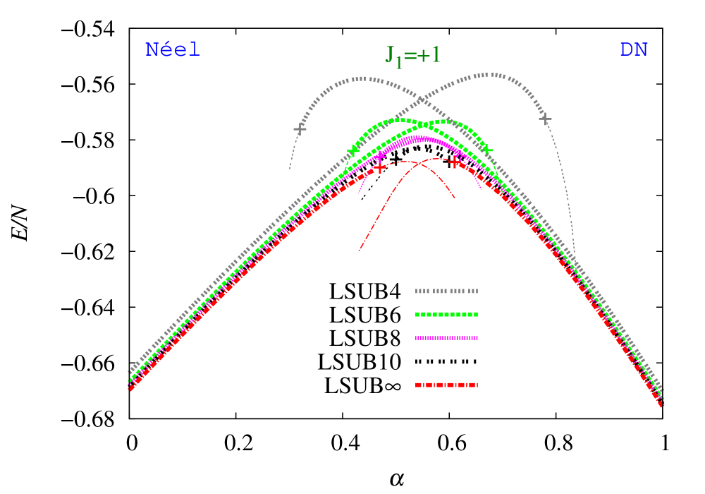
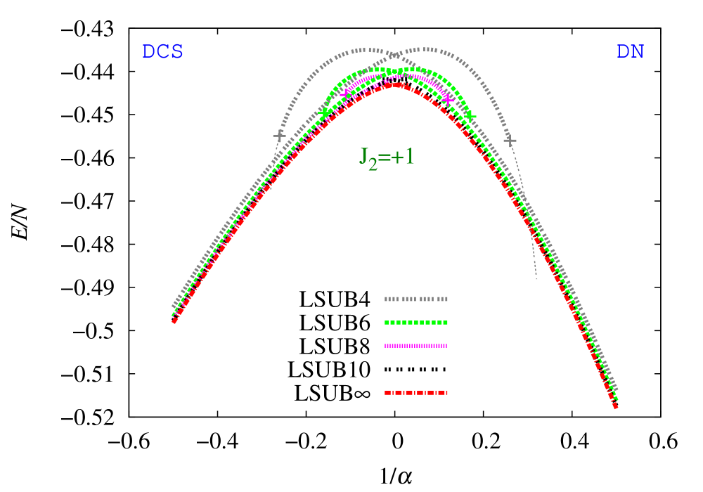
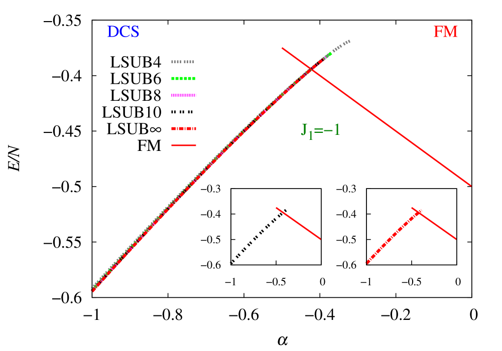
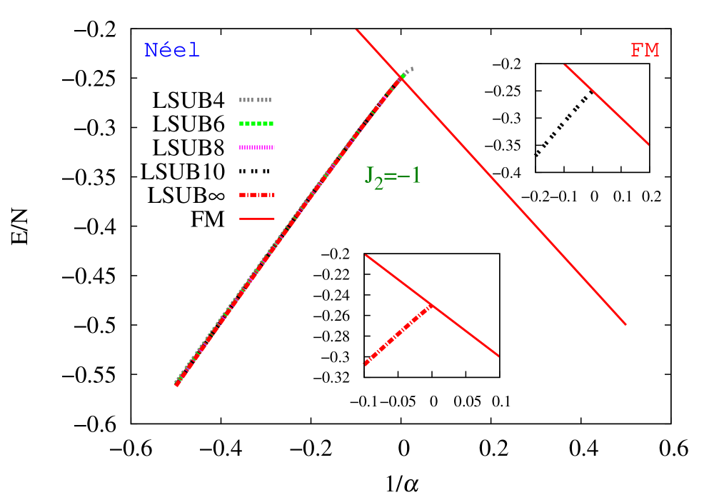
Figure 2: (Color online) CCM LSUB$m$ results with $m=\{4,6,8,10\}$ for the GS energy per spin, $E/N$, as a function of the frustration parameter, $\alpha\equiv J_{2}/J_{1}$, for the spin-1/2 $J_{1}$–$J_{2}$ model on a cross-striped square lattice, for the cases: (a) $J_{1}=+1$ and $0\leq\alpha\leq 1$, showing results based on both the Néel (left curves) and DN (right curves) states as model states; (b) $J_{2}=+1$ and $-0.5\leq\alpha^{-1}\leq 0.5$, showing results based on both the DCS (left curves) and DN (right curves) states as model states; (c) $J_{1}=-1$ and $-1\leq\alpha\leq 0$, showing results based on the DCS state (left curves) as model state, as well as the exact FM result (right solid curve), $E^{\rm FM}/N=-\frac{1}{4}(2+\alpha)$; and (d) $J_{2}=-1$ and $-0.5\leq\alpha^{-1}\leq 0.5$, showing results based on the Néel state (left curves) as model state, as well as the exact FM result (right solid curve), $E^{{\rm FM}}/N=-\frac{1}{4}(1+2/\alpha)$. In each case we also show the extrapolated LSUB$\infty$ result obtained from Eq. (4) using the data set $m=\{4,6,8,10\}$. All LSUB$m$ solutions are shown out to their respective (approximately determined) termination points. In Figs. 2(a) and 2(b) the plus ($+$) symbols mark the points where the respective solutions have $M\rightarrow 0$, and those portions of the curves beyond the plus ($+$) symbols shown with thinner lines indicate the respective unphysical regions where $M<0$ (and see text for details).

Firstly, in Fig. 2(a), results for the case $J_{1}>0$ are presented based on both the Néel and DN states. We note that for both model states results are shown only for certain ranges of the frustration parameter. Both sets of curves show a termination point, an upper one for the Néel curves and a lower one for the DN curves. These CCM LSUB$m$ termination points themselves depend on the truncation parameter, $m$. In general we find that the higher is the index $m$, the smaller is the range of values of $\alpha$ over which the corresponding (real) GS solution exists based on a particular model state.

Such terminations of CCM solutions are commonly found and are very well understood (see, e.g., Refs. Fa:2004, ; Bi:2009_SqTriangle, ; Bishop:2010_UJack, ). They are always reflections of the true quantum phase transitions that are present in the system under study. At such termination points the solution to the corresponding CCM LSUB$m$ equations ceases to be real, and beyond these points only two unphysical branches of complex conjugate solutions exist. On the other hand, in the region before any such termination point where the true physical solution is real, there actually must also exist another (unstable) real solution. Such other solutions are themselves both unphysical and, fortunately, also very difficult to determine numerically in general. In practice any simple numerical procedure will pick up only the physical branch, which itself is usually easy to identify by following it (as a function of the frustration parameter, $\alpha$, for example) to some appropriate asymptotic limit where it becomes exact or otherwise known.

The two (i.e., the physical and unphysical) real branches of solution thus meet at a termination point, beyond which they diverge again in the complex plane as wholly unphysical complex conjugate pairs. The values, $\alpha^{t}(m)$ of the termination points for a given branch of CCM LSUB$m$ solutions, may themselves actually be used to estimate the corresponding QCP for the GS phase under study, as $\alpha^{c}=\lim_{m\rightarrow\infty}\alpha^{t}(m)$. However, it comes as no surprise that the number of iterations required to solve the CCM LSUB$m$ equations, at a given level of accuracy, increases significantly as $\alpha\rightarrow\alpha^{t}(m)$. Hence, it is computationally expensive to obtain the values $\alpha^{t}(m)$ with high precision, and since we have accurate other means available, as described below, to determine the QCPs, we do not make use of this method here.

Returning to our discussion of Fig. 2(a), we often find (as is the case here), that for a region near $\alpha^{t}(m)$ on the corresponding real physical branch the solution itself is also unphysical in the sense that the corresponding order parameter (here the local on-site magnetization, $M$) takes negative values. These values where $M\rightarrow 0$ (determined as discussed in detail below) are shown both for the individual LSUB$m$ solutions and the corresponding LSUB$\infty$ extrapolations as plus ($+$) signs in Fig. 2(a), and the corresponding regions beyond these points where $M<0$ are shown with corresponding thinner curves than the regions marked with thicker curves where $M>0$. Two points are particularly noteworthy concerning Fig. 2(a). Firstly, whereas the corresponding LSUB$m$ branches of solutions, based on both the Néel and DN states as CCM model states, cross at a relatively sharp angle (as in the classical case, $s\rightarrow\infty$) for smaller values of the truncation parameter $m$, the angle becomes much shallower as $m$ increases. Thus, there are strong preliminary indications that the counterpart in the $s=\frac{1}{2}$ model of the classical first-order transition in Fig. 1(d) at $\theta^{{\rm cl}}_{1}=\tan^{-1}(\frac{1}{2}$) might become second-order. Secondly, it is also apparent from Fig. 2(a) that the overlap region where CCM LSUB$m$ solutions, for a given value of $m$, exist for both the Néel and DN phases becomes smaller as $m$ increases. Indeed, for the LSUB$\infty$ extrapolation a clear gap has opened around $\alpha\approx 0.5$ where neither the Néel or the DN phase exists. We discuss this interesting regime in much greater detail below.

Before turning to our CCM results based on other model states, it is worth commenting briefly on the overall accuracy of our results. To do so we may, in particular, examine the special case for $J_{1}=+1$ of $\alpha=0$ (i.e., $\theta=0$), corresponding to the Néel order of the square-lattice HAF. Thus, our extrapolated LSUB$\infty$ result for the GS energy per spin based on our LSUB$m$ results with $m=\{4,6,8,10\}$ and using the Néel state as CCM model state for this case $\theta=0$, is $E/N\approx-0.66973$. This may be compared, for example, with the corresponding results for the spin-1/2 square-lattice HAF, $E/N=-0.6693(1)$ from a linked-cluster series expansion techniqueZh:1991 , and $E/N=-0.669437(5)$ from a large-scale QMC simulation,Sa:1997 free of the usual “minus-sign-problems” for this special (unfrustrated limiting) case where the Marshall-Peierls sign ruleMa:1955 may be applied. Our own CCM result is thus in remarkably good agreement with these benchmark results for this particular case. We have no reason to believe that similar accuracy does not pertain over the entire phase diagram. Finally, it is worth noting too that our extrapolated result is extremely robust with respect to the choice of LSUB$m$ data set used to obtain it. For example, use of the data sets $m=\{6,8,10\}$ and $m=\{4,6,8\}$ in Eq. (4) yields the corresponding respective results at $\theta=0$ of $E/N\approx-0.66967$ and $E/N\approx-0.66977$. Even inclusion of the very low-order LSUB2 result with $m=\{2,4,6,8\}$ yields $E/N\approx-0.66981$.

In Fig. 2(b) we show the corresponding energy results for both the DCS and DN phases in the region $J_{2}=+1$ around $\theta=\frac{1}{2}\pi$ where they meet in the classical ($s\rightarrow\infty$) version of the model, as shown in Fig. 1(d). Once again, it is clear that the overlap region where both CCM solutions exist at a given LSUB$m$ level decreases as the truncation index $m$ increases. Secondly, just as in Fig. 2(a), the crossing angle of the two curves at $\alpha^{-1}=0$ becomes much shallower as $m$ increases, again more indicative of a continuous (second-order) transition than the corresponding first-order transition in the classical ($s\rightarrow\infty$) version of the model.

The crossing point at $J_{1}=0$ (with $J_{2}=+1$) of each of the pairs of LSUB$m$ curves based on the DCS and DN states as CCM model states is precisely the limiting case of decoupled 1D HAF $J_{2}$ chains. Hence, it is again interesting to ascertain the accuracy of our results by comparison with the exact results in this soluble limit. Thus, our extrapolated LSUB$\infty$ result for the GS energy per spin, based on either the DCS or DN model state, for this case $\theta=\frac{1}{2}\pi$ (with $J_{2}=+1$), and using the extrapolation scheme of Eq. (4) with $m=\{4,6,8,10\}$, is $E/N\approx-0.44312$. Again, our results are remarkably robust with respect to the choice of LSUB$m$ data set used. Thus, for example, use of the data sets $m=\{6,8,10\}$ and $m=\{4,6,8\}$ in Eq. (4) yields the corresponding results at $\theta=\frac{1}{2}\pi$ of $E/N\approx-0.44313$ and $E/N\approx-0.44311$, respectively. Even inclusion of the very low-order LSUB2 result with $m=\{2,4,6,8\}$ yields $E/N\approx-0.44308$. Thus, once again, our CCM results are seen to be in excellent agreement with the corresponding exact result, $E/N=\frac{1}{4}-\ln 2\approx-0.44315$, from the Bethe ansatz solution.Bethe:1931 ; Hulthen:1938

Let us now turn to the case $J_{1}=-1$. In Fig. 2(c) we show our CCM results based on the DCS state as model state in this region. We note first that over the entire regime shown the LSUB$m$ results converge extremely rapidly as the order $m$ increases. Secondly, we note too that the LSUB$m$ termination points also similarly converge rather fast, and approach the crossing point with the exact FM eigenstate. This is explicitly shown in the inset for the LSUB10 case. The crossing point of the LSUB$\infty$ DCS curve with the FM curve is now at the value $\alpha=-0.423(1)$, irrespective of which LSUB$m$ data set is used to perform the extrapolation.

With respect to the GS energy, finally we show in Fig. 2(d) our results based on the Néel state in the unfrustrated region where $J_{2}<0$. As in the previous case of Fig. 2(c), the LSUB$m$ results again converge very rapidly as the truncation order parameter $m$ increases. Similarly too, the LSUB$m$ termination points converge very rapidly to precisely the point $J_{1}=0$ where all of our energy results cross that of the exact FM eigenstate, which is also shown in Fig. 2(d), as can be explicitly seen in the inset to the figure for the LSUB10 case.

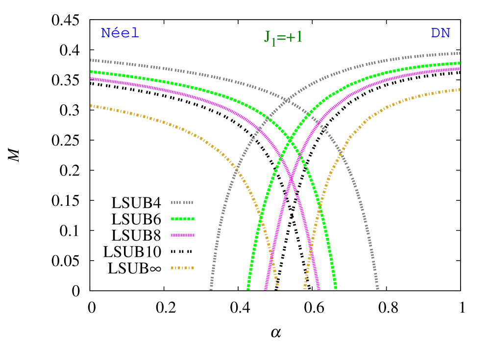
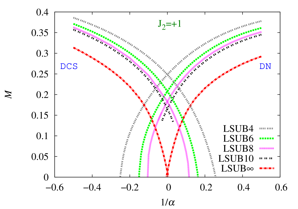
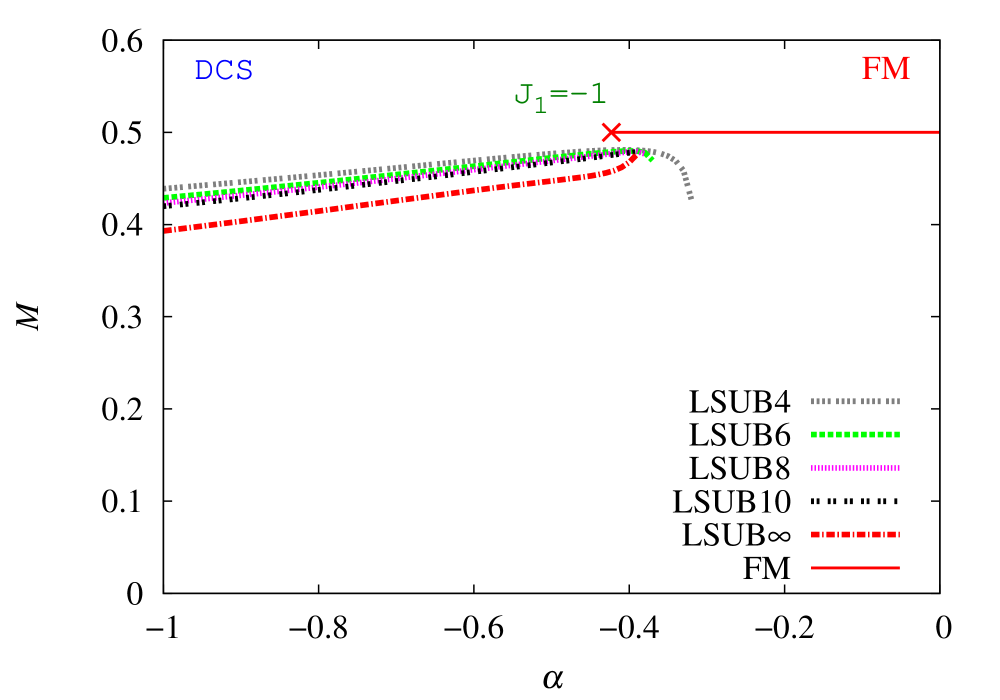
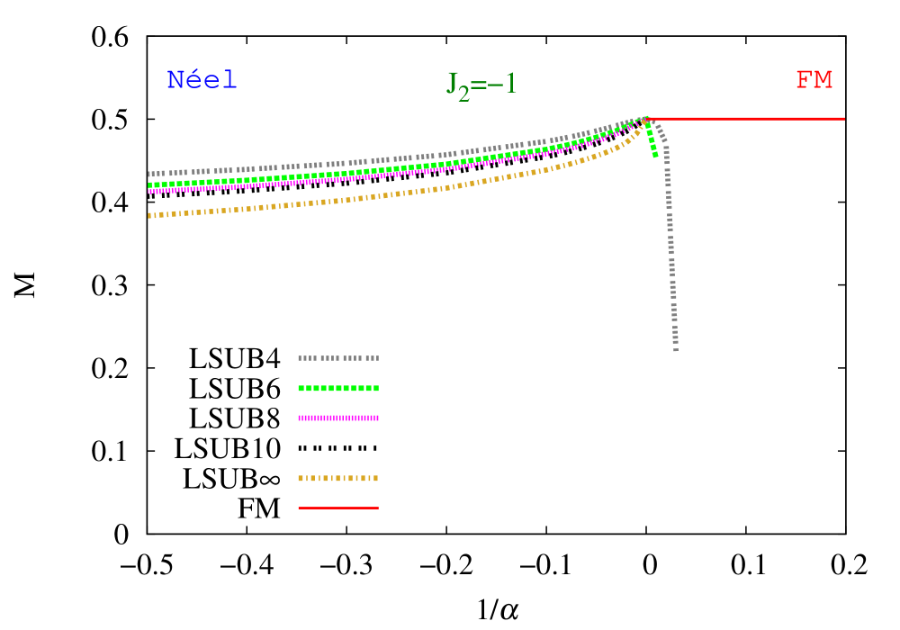
Figure 3: (Color online) CCM LSUB$m$ results with $m=\{4,6,8,10\}$ for the magnetic order parameter, $M$, as a function of the frustration parameter, $\alpha\equiv J_{2}/J_{1}$, for the spin-1/2 $J_{1}$–$J_{2}$ model on a cross-striped square lattice, for the cases: (a) $J_{1}=+1$ and $0\leq\alpha\leq 1$, showing results based on both the Néel (left curves) and DN (right curves) states as model states; (b) $J_{2}=+1$ and $-0.5\leq\alpha^{-1}\leq 0.5$, showing results based on both the DCS (left curves) and DN (right curves) states as model states; (c) $J_{1}=-1$ and $-1\leq\alpha\leq 0$, showing results based on the DCS state (left curves) as model state, as well as the exact FM result (right solid curve), $M^{\rm FM}=\frac{1}{2}$; and (d) $J_{1}=-1$ and $-0.5\leq\alpha^{-1}\leq 0.2$, showing results based on the Néel state (left curves) as model state, as well as the exact FM result (right solid curve), $M^{{\rm FM}}=\frac{1}{2}$. In each case we also show the extrapolated LSUB$\infty$ result obtained by inputting the data set $m=\{4,6,8,10\}$ into Eq. (5) for cases (a) and (d) and into Eq. (6) for cases (b) and (c). The cross ($\times$) symbol in Fig. 3(c) marks the position of the corresponding energy crossing point in Fig. 2(c).

To summarize our results obtained from the energy calculations, we have found strong definite evidence so far of five QCPs, four in the frustrated region where $J_{2}>0$ and one in the unfrustrated region where $J_{2}<0$. Firstly, in the (frustrated) first quadrant of the phase diagram where $J_{1}>0$ and $J_{2}>0$, the classical critical point at $\alpha^{{\rm cl}}_{1}=\frac{1}{2}$ appears to be split into two QCPs in the $s=\frac{1}{2}$ case at positions $\alpha^{c}_{1a}\lesssim 0.5$ and $\alpha^{c}_{1b}\approx 0.6$, with a Néel-ordered GS phase for $\alpha<\alpha^{c}_{1a}$, a DN-ordered GS phase for $\alpha>\alpha^{c}_{1b}$, and an as yet unknown intermediate phase. Secondly, we find that the spin-1/2 and classical versions of the model share a common critical point at $J_{1}=0$ when $\theta^{c}_{2}=\frac{1}{2}\pi=\theta^{{\rm cl}}_{2}$, at which the DN-ordered GS phase for values $J_{1}>0$ yields to the DCS-ordered GS phase for values $J_{1}<0$. However, unlike the classical first-order transition at this point, its $s=\frac{1}{2}$ quantum analog seems to be more second-order in character in terms of the energy results. Thirdly, in the (frustrated) second quadrant of the phase diagram where $J_{1}<0$ and $J_{2}>0$, the classical critical point at $\alpha^{{\rm cl}}_{3}=-\frac{1}{2}$, at which the DCS-ordered GS phase yields to the FM-ordered GS phase, is shifted in the $s=\frac{1}{2}$ case to a QCP at $\alpha^{c}_{3}=-0.423(1)$. Finally, in the (unfrustrated) lower hemisphere of the phase diagram where $J_{2}<0$, we find, as expected, that the spin-1/2 and classical versions of the model share a common critical point at $J_{1}=0$ when $\theta^{c}_{4}=\frac{3}{2}\pi=\theta^{{\rm cl}}_{4}$ at which the FM-ordered GS phase for values $J_{1}<0$ yields to the Néel-ordered GS phase for values $J_{1}>0$.

In order to examine the nature of these QCPs in more detail, and especially the positions of the two QCPs at $\alpha^{c}_{1a}$ and $\alpha^{c}_{1b}$, we now turn our attention to our corresponding results for the GS order parameter $M$. Our LSUB$m$ results with $m=\{4,6,8,10\}$ using each of the previous CCM model states are shown in Fig. 3.

Figure 3(a) presents the analogous results for $M$ based on both the Néel and DN states as shown in Fig. 2(a) for the GS energy, applicable to the (frustrated) first quadrant of the phase diagram with $J_{1}>0$ and $J_{2}>0$. The plus ($+$) symbols shown in Fig. 2(a) for the LSUB$m$ results presented there correspond to the respective points in Fig. 3(a) at which $M=0$.

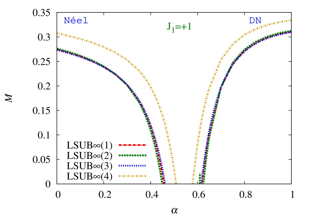
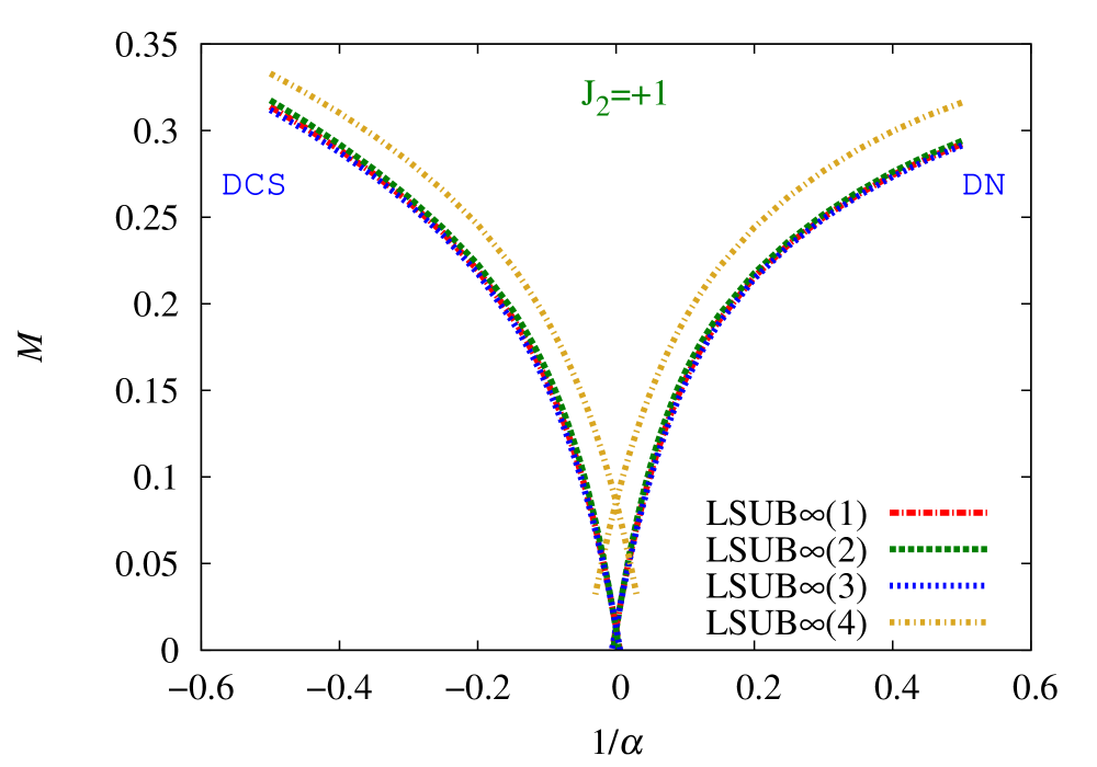
Figure 4: (Color online) Various extrapolated CCM LSUB$\infty$ results for the magnetic order parameter, $M$, as a function of the frustration parameter, $\alpha\equiv J_{2}/J_{1}$, for the spin-1/2 $J_{1}$–$J_{2}$ model on a cross-striped square lattice, for the cases: (a) $J_{1}=+1$ and $0\leq\alpha\leq 1$, showing results based on both the Néel (left curves) and DN (right curves) states as model states; (b) $J_{2}=+1$ and $-0.5\leq\alpha^{-1}\leq 0.5$, showing results based on both the DCS (left curves) and DN (right curves) states as model states. The curves LSUB$\infty(k)$ with $k=1,2,3$ use the extrapolation scheme of Eq. (6) with LSUB$m$ data sets respectively: $k=1$, $m=\{4,6,8,10\}$; $k=2$, $m=\{6,8,10\}$; and $k=3$, $m=\{4,6,8\}$; while the curve LSUB$\infty(4)$ uses the extrapolation scheme of Eq. (5), with LSUB$m$ data set $m=\{4,6,8,10\}$.

In order to consider again the special case for $J_{1}=+1$ of $\alpha=0$, corresponding to the Néel order of the square-lattice HAF, we also show in Fig. 3(a) the extrapolated LSUB$\infty$ result for the order parameter $M$ based on our LSUB$m$ results for the Néel model state with $m=\{4,6,8,10\}$ used in the scheme of Eq. (5), which is applicable for this unfrustrated limiting case. Our corresponding estimate for the square-lattice HAF is then $M\approx 0.307$. This may again be compared with the corresponding result $M=0.307(1)$ from a linked-cluster series expansion technique,Zh:1991 and $M=0.3070(3)$ from a large-scale quantum Monte Carlo simulation.Sa:1997 Once again we may demonstrate the robustness of our extrapolation by comparing results obtained from the use of different data sets. For example, use of the data sets $m=\{6,8,10\}$ and $m=\{4,6,8\}$ in Eq. (5) yields the corresponding respective results at $\theta=0$ of $M\approx 0.305$ and $M\approx 0.309$. Even inclusion of the very low-order LSUB2 result into the set $m=\{2,4,6,8\}$ still gives the extremely good result $M\approx 0.314$.

We have shown the LSUB$\infty$ extrapolated values for $M$ in Fig. 3(a) using the scheme of Eq. (5), since we wished primarily to use it to determine the accuracy of our technique at the special unfrustrated point $\alpha=0$ where this scheme is especially appropriate. However, when we now turn our attention to the very interesting QCPs at $\alpha^{c}_{1a}$ and $\alpha^{c}_{1b}$ the extrapolation scheme of Eq. (5) loses its validity, and instead the scheme of Eq. (6) becomes apposite. Nevertheless, Fig. 2(a) shows clearly that even use of the scheme of Eq. (5) gives clear indications of a gap between the Néel and DN phases, which can only widen when the more appropriate scheme of Eq. (6) is used in this critical regime.

Thus, in Fig. 4(a) we now show the corresponding extrapolated results using the scheme of Eq. (6), and where we also demonstrate the robustness of our fitting procedure by using various LSUB$m$ data sets to perform the fits. The use of such a sensitivity analysis as shown in Fig. 4(a) yields values for the corresponding QCPs, $\alpha^{c}_{1a}=0.46(1)$ and $\alpha^{c}_{1b}=0.62(1)$.

The results shown in both Figs. 3(b) and 4(b) also show very clearly the phase transition between the DCS and DN phases at $\theta^{c}_{2}=\frac{1}{2}\pi$. In particular, Fig. 4(b) demonstrates that when the extrapolation scheme of Eq. (6) is used, as is appropriate at the QCP, the order parameter $M$ becomes zero within extremely small error bars on both sides of the transition precisely at the QCP, thereby adding considerable weight to the conclusion from the GS energy results that this transition is a (continuous) second-order one, quite unlike its classical first-order counterpart.

It is worth emphasizing that, although we show in Fig. 4(b) extrapolations based on both Eqs. (5) and (6), for the sake of comparison and completeness, the proper choice in this case is most definitely Eq. (6) for reasons stated above and in Sec. III. Furthermore, as we have indicated, in any such analysis we may also use Eq. (7) for a first fit to the results, in order to find the leading exponent. In the case of the results shown in Fig. 4(b), for example, such a fit clearly shows that Eq. (6) is indeed the appropriate choice, fully as expected from much accumulated prior experience.

In Fig. 3(c) we show the corresponding CCM results for the order parameter to those shown in Fig. 2(c) for the GS energy, in the region where the DCS and FM phases meet. As discussed previously, the LSUB$m$ results based on the DCS state as model state terminate at points, depending on the truncation parameter $m$, that always extend slightly into the region where the FM state is the stable phase, but where the nonphysical region decreases as $m$ increases. The DCS termination point for the LSUB10 approximation is, for example, at a value $\alpha\approx-0.39$, and the corresponding extrapolated LSUB$\infty$ value, shown in Fig. 3(c), based on the extrapolation scheme of Eq. (6), also terminates at this value. For comparison, the cross ($\times$) symbol in Fig. 3(c) on the FM curve, $M^{{\rm FM}}=\frac{1}{2}$, marks the position, $\alpha\approx-0.423$, of the corresponding energy crossing point from Fig. 2(c). It seems clear that if we could go to arbitrarily high LSUB$m$ orders in this case the DCS order parameter would approach the value 0.5 with a similar cusp shape as in our approximate LSUB$\infty$ result in Fig. 3(c) at precisely the energy crossing point, namely $\alpha^{c}_{3}$. For this particular transition, the energy results clearly give a more accurate estimate for $\alpha^{c}_{3}$ than the order parameter results.

Finally, with respect to the magnetic order parameter, we show in Fig. 3(d) the corresponding CCM results for the Néel phase in the region where it meets the FM phase. The appropriately extrapolated LSUB$\infty$ result shows clearly how $M$ approaches the value 0.5 on the Néel side with a similar cusp to that observed in Fig. 3(c).

Clearly, our results for $M$ completely reinforce the conclusions we have already drawn from our corresponding results for the GS energy. Taken together they give clear evidence for the quantum $s=\frac{1}{2}$ model to contain five phases in the GS phase diagram, by contrast with the four phases of its classical ($s\rightarrow\infty$) counterpart. We have also found accurate values for all five QCPs. What remains unclear up till now, however, is the nature of the phase in the regime $\alpha^{c}_{1a}<\alpha<\alpha^{c}_{1b}$. In order to shed light on this remaining issue we now investigate the susceptibility of our CCM solutions in this regime to various forms of valence-bond crystalline (VBC) order.

Two obvious forms of VBC order to consider in this context are the plaquette valence-bond crystalline (PVBC) and crossed-dimer valence-bond crystalline (CDVBC) forms illustrated in Figs. 5(a) and (b) respectively.

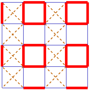
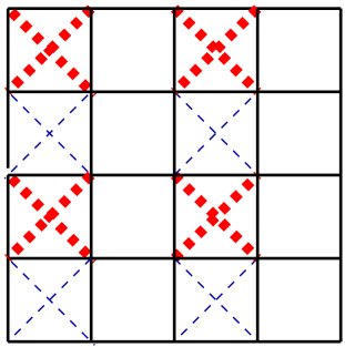
Figure 5: (Color online) The fields (or perturbations), $F=\delta\;\hat{O}$, for the two forms of valence-bond crystalline (VBC) susceptibility considered, namely: (a) plaquette (PVBC), $\chi_{p}$; and (b) crossed-dimer (CDVBC), $\chi_{d}$. In case (a) the thick (red) and thin (blue) solid lines correspond respectively to strengthened and weakened $J_{1}$ exchange couplings, where $\hat{O}_{p}=\sum_{\langle i,j\rangle}a_{ij}\mathbf{s}_{i}\cdot\mathbf{s}_{j}$, and the sum runs over all NN bonds of the square lattice, with $a_{ij}=+1$ and $-1$ for thick (red) and thin (blue) lines respectively, as shown. In case (b) the thick (red) and thin (blue) dashed lines correspond respectively to strengthened and weakened $J_{2}$ exchange couplings, where $\hat{O}_{d}=\sum_{\langle\langle i,k\rangle\rangle^{\prime}}a_{ik}\mathbf{s}_{i}\cdot\mathbf{s}_{k}$, and the sum runs over all diagonal bonds of the cross-striped square lattice, with $a_{ik}=+1$ and $-1$ for thick (red) and thin (blue) dashed lines respectively. The original solid (black) $J_{1}$ bonds and dashed (brown) $J_{2}$ bonds are unaltered in strength.

For both cases we simply consider the response of the system when a corresponding field operator, $F=\delta\;\hat{O}$, is added as a small perturbation to the original Hamilton of Eq. (1), with $\delta$ an infinitesimally small $c-$number.darradi08 The particular operators $\hat{O}_{p}$ and $\hat{O}_{d}$, corresponding respectively to PVBC and CDVBC ordering, are illustrated graphically in Figs. 5(a) and (b) and are also defined explicitly in the caption.

In both cases we calculate the perturbed GS energy per spin, $e(\delta)\equiv E(\delta)/N$, for the perturbed Hamiltonian $H+F$, at various LSUB$m$ levels of approximation. We use the Néel and DN states as CCM model states since we are especially interested in the phase intermediate between them in the spin-1/2 phase diagram. We then calculate the corresponding susceptibility,

$$\chi\equiv-\left.(\partial^{2}{e(\delta)})/(\partial{\delta}^{2})\right|_{\delta=0}\,,$$ (8)

and use it to find points or regions where the phase corresponding to the particular CCM model state used becomes unstable against the specified form of VBC order, namely when its extrapolated inverse susceptibility, $\chi^{-1}$, goes to zero.

Clearly our CCM LSUB$m$ results for any susceptibility still need to be extrapolated to the LSUB$\infty$ limit. The most straightforward way to do so Li:2013_chevron is clearly to extrapolate first our LSUB$m$ results for the perturbed energy using an unbiased scheme such as in Eq. (7),

$$e^{(m)}(\delta)=e_{0}(\delta)+e_{1}(\delta)m^{-\nu}\,,$$ (9)

with the exponent $\nu$ a fitting parameter, along with $e_{0}(\delta)$ and $e_{1}(\delta)$. Generally, as is to be expected from our standard LSUB$m$ energy extrapolation scheme of Eq. (4), the fitted value of $\nu$ is close to 2 for most values of the frustration parameter $\alpha$ pertaining to the particular CCM model state used, except very near (or inside) any critical regime, where it can deviate sharply from the value 2, as discussed in more detail below.

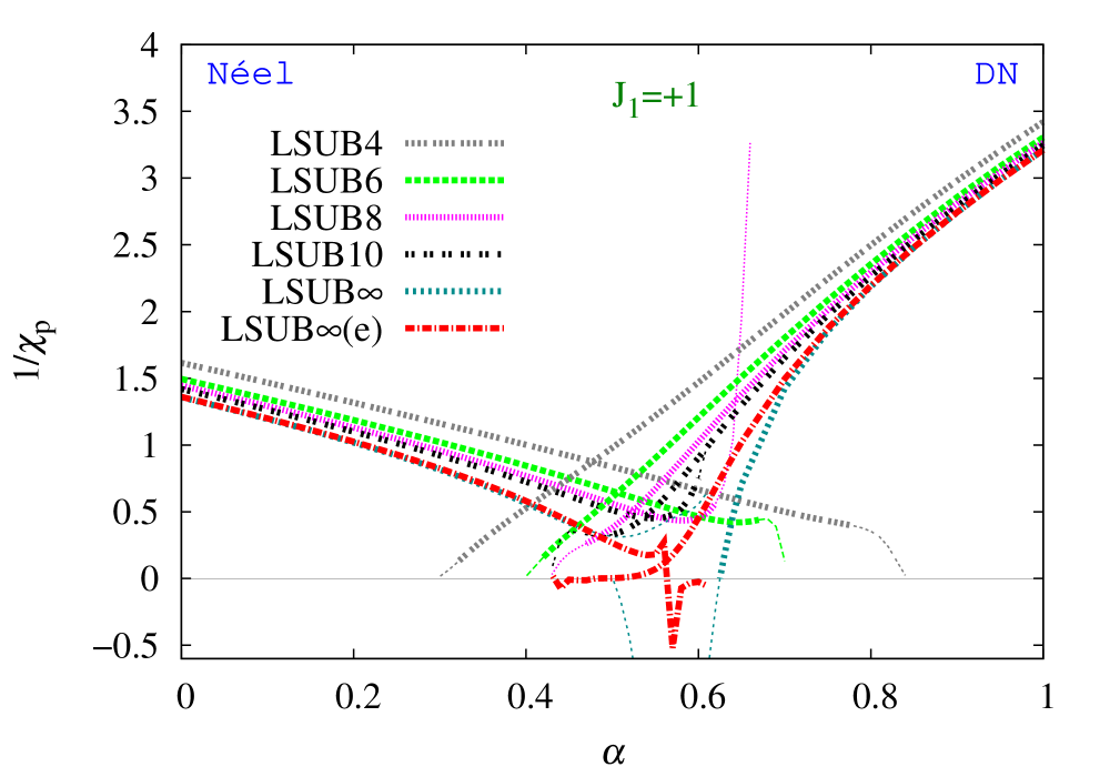
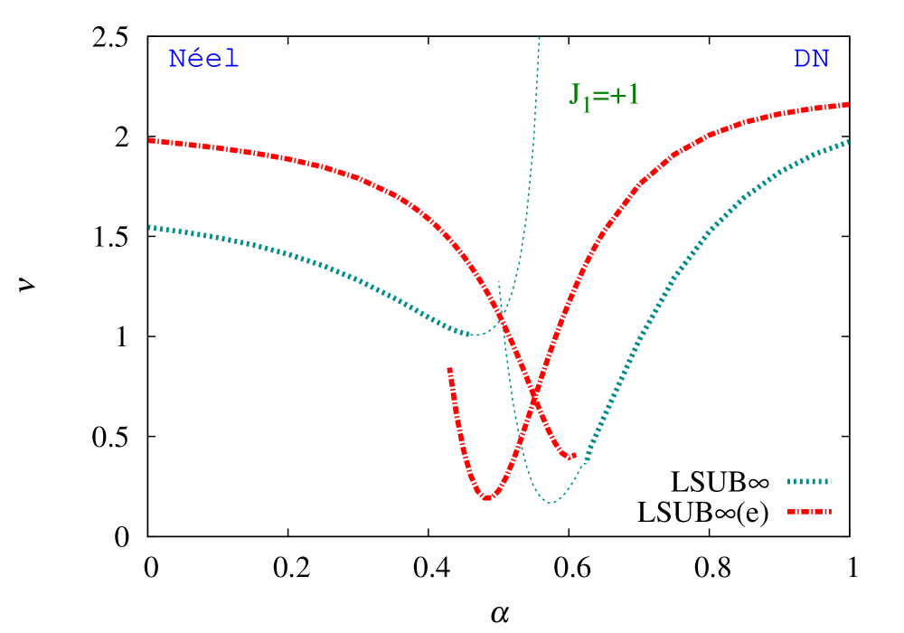
Figure 6: (Color online) (a) CCM results for the inverse plaquette susceptibility, $1/\chi_{{\rm p}}$, appropriate to the PVBC ordering of Fig. 5(a), as a function of the frustration parameter, $\alpha\equiv J_{2}/J_{1}$, for the spin-1/2 $J_{1}$–$J_{2}$ model (with $J_{1}=+1$) on a cross-striped square lattice, using both the Néel state (left curves) and DN state (right curves) as the CCM model state. For both model states we show the LSUB$m$ results with $m=\{4,6,8,10\}$, plus the corresponding extrapolated results LSUB$\infty$ and LSUB$\infty$(e) using this data set in the extrapolation schemes of Eqs. (12) and (9), respectively. Those portions of the curves with thinner lines indicate the respective unphysical regions where $M<0$ (and see text for details). Note that the LSUB$\infty$ curves are shown with thinner lines over the unphysical ranges, since the corresponding results for $1/\chi_{p}$ clearly behave non-monotonically there. By contrast, the LSUB$\infty$(e) curves are shown over the entire region where all of the LSUB$m$ approximations have real solutions (i.e., out to the respective termination points of the highest, LSUB10, solution), since the results for the perturbed energies used in this extrapolation behave monotonically almost everywhere the solutions exist. (b) The respective fitted values of the exponent $\nu$ in the extrapolation schemes of Eqs. (12) and (9), for the same fits as shown in Fig. 6(a) to the left.

We have also found previouslyDJJF:2011_honeycomb ; Li:2013_chevron that our LSUB$m$ values $\chi(m)$ may themselves very accurately be directly extrapolated to the $m\rightarrow\infty$ limit using the same scheme,

$$\chi(m)=d_{0}+d_{1}m^{-2}+d_{2}m^{-4}\,,$$ (10)

as for the GS energy itself in Eq. (4). A corresponding direct extrapolation of the more relevant quantity, the inverse susceptibility,

$$\chi^{-1}(m)=x_{0}+x_{1}m^{-2}+x_{2}m^{-4}\,,$$ (11)

has also been foundDJJF:2011_honeycomb ; Li:2013_chevron to give consistently good results, which agree well with those obtained from Eq. (10), although again with the exception of regions where $\chi^{-1}$ becomes very small or zero. Since we are here interested precisely in such regions over an extended range of values of the frustration parameters, $\alpha^{c}_{1a}\lesssim\alpha\lesssim\alpha^{c}_{1b}$, we may also use an unbiased extrapolation scheme of the form of Eq. (7),

$$\chi^{-1}(m)=y_{0}+y_{1}m^{-\nu}\,,$$ (12)

in such a case,DJJF:2011_honeycomb ; Li:2013_chevron where $y_{0}$, $y_{1}$, and $\nu$ are all treated as fitting parameters.

In Fig. 6(a) we present our results for the inverse plaquette susceptibility, $\chi^{-1}_{{\rm p}}$, pertaining to the PVBC ordering illustrated graphically in Fig. 5(a). We note that since the definition of $\chi$ is invariant with respect to the sign of the perturbation parameter $\delta$ in the case of PVBC order, its graphical definition in Fig. 5(a) is invariant with respect to interchange of the strengthened (thick, red) and weakened (thin, blue) $J_{1}$ bonds. We show explicitly in Fig. 6(a) our LSUB$m$ results based on both the Néel and DN states as CCM model states, with $m=\{4,6,8,10\}$, together with two extrapolated results, LSUB$\infty$ and LSUB$\infty$(e), based on Eqs. (12) and (9) respectively, and in each case using the respective data sets $m=\{4,6,8,10\}$ to perform the fits. What is especially noteworthy in the first place is how very close are the two different extrapolations for both the Néel and DN states as model states, except precisely in the region $\alpha^{c}_{1a}\lesssim\alpha\lesssim\alpha^{c}_{1b}$ where they have different forms. However, even in this most interesting region, the physical picture that emerges is a rather consistent one.

Thus, from the raw LSUB$m$ results themselves, we see clearly that both the Néel-ordered and DN-ordered states become highly susceptible to PVBC ordering around the same points at which their respective magnetic order parameters, $M$, approach zero, as in Fig. 3(a). On the Néel side, although the LSUB$\infty$ result for $\chi^{-1}_{p}$ based on Eq. (12) does not become exactly zero it does become very small around our previous estimates for $\alpha^{c}_{1a}$, and the corresponding LSUB$\infty$(e) result shows a clear minimum, with an even smaller value of $\chi^{-1}_{p}$, at a slightly larger value of $\alpha$, just before the extrapolation becomes unstable, in the region where the corresponding solutions are unphysical since (some of) the LSUB$m$ solutions have a value there of $M<0$, as seen from Fig. 3(a).

By contrast, the extrapolated results based on the DN state have markedly different character. Thus, the LSUB$\infty$ extrapolated result for $1/\chi_{p}$ based on Eq. (12) goes to zero at a value $\alpha=0.62(2)$, where the error bar is an estimate from using different LSUB$m$ data sets, as discussed previously. A close inspection of Fig. 6(a) reveals, however, that this LSUB$\infty$ result for $1/\chi_{p}$ based on the extrapolation scheme of Eq. (12) then becomes zero again as $\alpha$ is decreased further, at a value $\alpha\approx 0.50$. These two values are completely consistent with our previous estimates of the two QCPs marking the range, $\alpha^{c}_{1a}\leq\alpha\leq\alpha^{c}_{1b}$, of the intermediate phase, namely, $\alpha^{c}_{1b}=0.62(1)$ and $\alpha^{c}_{1a}=0.46(1)$. Even more revealing perhaps is the estimate LSUB$\infty$(e) for $1/\chi_{p}$, shown in Fig. 6(a), which is based on the most direct extrapolation scheme of Eq. (9). Here we observe very clearly that $1/\chi_{p}$ is zero (or very close to zero within the small error bars of the extrapolation) over a range $\alpha^{c}_{1a}\lesssim\alpha\lesssim\alpha^{c}_{1b}$. Thus, all of the evidence from our results from $\chi_{p}$ is compatible with the interpretation that the quantum phase intermediate between those with Néel and DN order has PVBC order.

In Fig. 6(b) we show the values of the exponent $\nu$ that we obtain from our LSUB$\infty$ and LSUB$\infty$(e) fits to the LSUB$m$ extrapolation schemes of Eqs. (12) and (9) respectively. The values shown are based on fitting to the LSUB$m$ data set $m=\{4,6,8,10\}$ for both the Néel and DN solutions. However, the fitted values are themselves again remarkably robust with respect to the choice of data set. Figure 6(b) shows that when $\chi_{p}$ is calculated using Eq. (9), the fitted value of the exponent $\nu$ is very close to the expected value 2, as in our standard GS energy extrapolation scheme of Eq. (4), except for values of $\alpha$ in the approximate range $\alpha^{c}_{1a}\lesssim\alpha\lesssim\alpha^{c}_{1b}$, where it drops sharply. In practice the second derivative of $e(\delta)$ required in Eq. (8) is calculated numerically using values $\delta=0,\pm d$, typically with $d=0.001$. The corresponding value of $\nu$ in Eq. (9) that are plotted in Fig. 6(b) are then essentially identical for these three values of $\delta$ that we use. On the other hand, when $1/\chi_{p}$ is calculated using Eq. (12) the fitted value for the exponent $\nu$ is close to 1.5 on the Néel side and 2 on the DN side, again except for values of $\alpha$ in the critical range $\alpha^{c}_{1a}\lesssim\alpha<\alpha^{c}_{1b}$, where they similarly deviate sharply. It is interesting to note that a value $\nu\approx 1.5$ has also been observed previously when using Eq. (12) for the extrapolations of $1/\chi_{p}$ for the Néel state in the related $J_{1}$–$J_{2}$ models on the checkerboard Bishop:2012_checkerboard and chevron-squareLi:2013_chevron lattices.

Although our results for $\chi_{p}$ provide very strong evidence for a PVBC-ordered GS phase intermediate between the Néel and DN GS phases for the quantum spin-1/2 model, we have also performed similar CCM calculations based on the Néel and DN states as model states for the corresponding crossed-dimer susceptibility, $\chi_{d}$, pertaining to the CDVBC order illustrated graphically in Fig. 5(b). The results for $\chi_{d}$ are qualitatively quite different to those for $\chi_{p}$. Thus, in the case of $\chi_{d}$ the extrapolated results show no indication at all of being zero (or unphysically negative) over any finite range. Instead, the DN and Néel results, respectively, for $1/\chi_{d}$ become zero (or very closely approach zero) only at single points, which are themselves completely compatible with our prior estimates for $\alpha^{c}_{1a}$ and $\alpha^{c}_{1b}$. Thus, while the results for $1/\chi_{d}$ corroborate our previous estimates for these two QCPs, they provide no evidence at all for any CDVBC-ordered phase, since $1/\chi_{d}$ does not vanish over any finite range of values of $\alpha$. The fact that $1/\chi_{d}$ vanishes at specific points, namely $\alpha^{c}_{1a}$ and $\alpha^{c}_{1b}$, simply reinforces these as being QCPs, since at any QCP one expects the system to become infinitely susceptible to all forms of ordering that are compatible with the symmetries of the physical and model states.

We now summarize our results in Sec. V.

V SUMMARY

We have investigated the complete $T=0$ GS phase diagram of an $s=\frac{1}{2}$ $J_{1}$–$J_{2}$ Heisenberg model on a cross-striped square lattice, for all values of $J_{1}$ and $J_{2}$, both positive and negative.

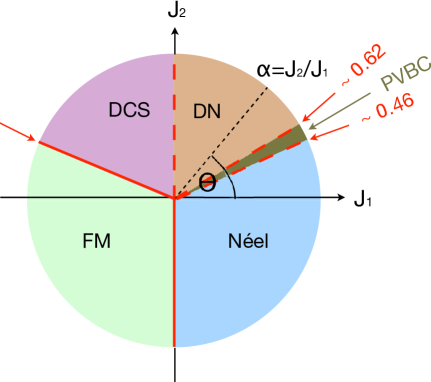
Figure 7: (Color online) The ground-state phase diagram of the spin-1/2 $J_{1}$–$J_{2}$ model on a cross-striped square lattice (with $\alpha\equiv\tan\theta\equiv J_{2}/J_{1}$), showing the three antiferromegnetic phases, namely Néel, double Néel (DN) and double columnar striped (DCS), illustrated in Figs. 1(a)–(c) respectively; the plaquette valence-bond crystalline (PVBC) phase illustrated in Fig. 5(a); and the ferromagnetic (FM) phase. The three transitions at $\alpha^{c}_{1a}=0.46(1)$ and $\alpha^{c}_{1b}=0.62(1)$, which mark the boundaries of the PVBC phase, and at $\theta^{c}_{2}=\frac{1}{2}\pi$ between the DN and DCS phases, all with $J_{2}>0$, each shown by a broken line, all appear to be continuous ones; while the two transitions at $\alpha^{c}_{3}=-0.423(1)$ (with $J_{2}>0$) and at $\theta^{c}_{4}=\frac{3}{2}\pi$, which mark the boundaries of the FM phase, both shown by solid lines, are first-order ones.

The classical ($s\rightarrow\infty$) version of the model has four GS phases, as illustrated in Fig. 1(d), with each of the corresponding phase transitions of first-order type. In the first quadrant of the phase diagram (where $J_{1}\geq 0$ and $J_{2}\geq 0$) the model interpolates continuously between a 2D HAF on the square lattice (when $J_{2}/J_{1}\equiv\alpha=0$) and uncoupled 1D HAF chains (as $\alpha\rightarrow\infty$). For the spin-1/2 quantum model we have found a GS phase diagram with five phases, with our main findings summarized in Fig. 7.

One of our main conclusions is that the classical direct first-order transition between the AFM Néel and DN phases at $\alpha^{{\rm cl}}_{1}=0.5$ (with $J_{1}>0$) is split into two transitions in the $s=\frac{1}{2}$ case, with QCPs at $\alpha^{c}_{1a}=0.46(1)$ and $\alpha^{c}_{1b}=0.62(1)$, and an intermediate quantum phase with PVBC ordering. From the shape of the order-parameter curves in Fig. 3(a) it seems probable that both transitions are continuous, since a first-order transition is usually signalled by a much steeper (or discontinuous) fall to zero.DJJF:2011_honeycomb The shape of the corresponding curves for $1/\chi_{p}$ in Fig. 6(a) also corroborates that the transitions are continuous, since first-order ones also usually show a similar steep (or discontinuous) drop to zero.DJJF:2011_honeycomb Since the three phases, Néel, DN and PVBC, break different symmetries our results thus favour the deconfinement scenario for both transitions at $\alpha^{c}_{1a}$ and $\alpha^{c}_{1b}$. Nevertheless, we should mention that generic arguments have been givenKuklov:2008 that phase transitions in models with SU(2)-symmetric deconfined critical points should be of first-order type. However, these arguments are based on effective field theories, while our own calculations are based directly on the lattice model itself. Although we can never entirely exclude the possibility of the transitions at $\alpha^{c}_{1a}$ and $\alpha^{c}_{1b}$ being sufficiently weak first-order ones, our evidence points more clearly to them being of second-order (deconfined, continuous) type. While our most accurate determination of both $\alpha^{c}_{1a}$ and $\alpha^{c}_{1b}$ comes from the magnetic order parameter results shown in Figs. 3(a) and 4(a) as the respective points where Néel order and DN order melt, our results for $1/\chi_{p}$ shown in Fig. 6(a) strongly corroborate that these are the same points where PVBC order turns on. Naturally, we cannot entirely exclude, from our results as shown in Fig. 6(a), the possibility of a very narrow regime within the range $\alpha^{c}_{1a}<\alpha<\alpha^{c}_{1b}$ where yet another phase with a different form of ordering exists.

We appreciate that the evidence presented here for the transitions at $\alpha^{c}_{1a}$ and $\alpha^{c}_{1b}$ being of the continuous (deconfined) type is relatively weak and rather far from being conclusive. Nevertheless, we believe that the analysis is certainly sufficiently suggestive to justify further work to clarify the nature of these transitions, for example, by the calculation of critical exponents or by finding a positive signal of the emergent [U(1)] symmetry. Such calculations, however, have scarcely ever hitherto been attempted within the CCM framework itself, and are certainly beyond the scope of the present study in any case.

We have found, as expected, that the third QCP at $\theta^{c}_{3}=\frac{1}{2}\pi$ between the DN and DCS phases, coincides with the corresponding classical transition, $\theta^{{\rm cl}}_{3}=\frac{1}{2}\pi$. However, we have found very strong evidence, from both the GS energy results shown in Fig. 2(b) and the magnetic order parameter results shown in Figs. 3(b) and 4(b), that the quantum transition for the $s=\frac{1}{2}$ model is again a continuous second-order one (and hence, again, presumably a deconfined transition), by contrast with the first-order nature of this transition in the classical ($s\rightarrow\infty$) model.

On the other hand, the remaining two transitions that mark the boundaries of the FM phase, are clearly first order in both the $s=\frac{1}{2}$ and $s\rightarrow\infty$ cases. However, we have found that quantum fluctuations act to stabilize the collinear AFM order of the DCS phase to higher values of the corresponding frustration (i.e., here, to larger values of $\alpha^{-1}$, since the $J_{1}$ bonds now act to frustrate the AFM order of the $J_{2}$ chains) than in the classical case. Thus, we found that the classical transition at $\alpha^{{\rm cl}}_{3}=-0.5$ (with $J_{1}>0$) shifts by quantum fluctuations in the $s=\frac{1}{2}$ case to $\alpha^{c}_{3}=-0.423(1)$, where our best estimate for $\alpha^{c}_{3}$ now comes from the energy crossing point shown in Fig. 2(c). Such stabilization by quantum fluctuations of collinear AFM order at the expense of FM order in frustrated regions has been observed elsewhere, for example, in both the FM version of the full (undepleted) spin-1/2 $J_{1}$–$J_{2}$ model on the square latticerichter10:J1J2mod_FM and in a related model on the honeycomb lattice.Bishop:2012_honey_phase

Lastly, in the unfrustrated regime where $J_{2}<0$, the final QCP between the FM and the Néel phases has been found to occur at $\theta^{c}_{4}=\frac{3}{2}\pi$, at precisely the same place as the corresponding classical transition, $\theta^{{\rm cl}}_{4}=\frac{3}{2}\pi$, fully as expected.

As final point, it may be worthwhile to comment on the limitations of the present CCM formalism in this context. While there exists a large amount of strong evidence that the method can very accurately capture the properties and phase boundaries of (magnetically) ordered states of highly frustrated quantum magnets, the available evidence for its ability to capture phases that are not adiabatically connected to a chosen reference state is mixed. On the one hand there is considerable evidence, including from the present study, that the CCM can well describe the phase boundaries of such states as those without magnetic order but with various forms of VBC order, even when using a reference state with magnetic order that is not itself the stable GS phase in the region (or, indeed, anywhere). On the other hand, and in common with many other methods, the CCM does not easily detect directly such disordered phases as spin-liquid phases, e.g., of the topological spin-liquid type or the sliding Luttinger liquid (SLL) type mentioned in Sec. II. What the CCM can perhaps most easily provide in such circumstances is strong evidence for a region in the ($T=0$) GS phase diagram of a phase of a type for which one may then test by other means. In other words, in such circumstances, it is better suited to exclude possibilities and/or to provide signals for the existence of some (as yet unknown) phase. For example, for the present model it is conceivable that an SLL might, a priori, exist at high enough (but still finite) values of $\alpha$. However, as we have seen, no indications emerge from the present analysis that would lend credence to, or would justify a search for, such an SLL phase as a stable GS phase.

In conclusion, we have seen that the $J_{1}$–$J_{2}$ Heisenberg model on the cross-striped square lattice provides a challenging model with a rich GS phase diagram in the extreme $s=\frac{1}{2}$ quantum case, with several features that differ markedly from its classical ($s\rightarrow\infty$) counterpart. The application of other theoretical techniques to the model would hence surely be of interest, in order to confirm our results. It might also be interesting to examine the $s=1$ version of the model for further differences.

References

- (1) Quantum Magnetism, Lecture Notes in Physics Vol. 645, edited by U. Schollwöck, J. Richter, D. J. J. Farnell, and R. F. Bishop (Springer-Verlag, Berlin, 2004).
- (2) Frustrated Spin Systems, edited by H. T. Diep (World Scientific, Singapore, 2005).
- (3) S. Sachdev, Quantum Phase Transitions (Cambridge University Press, Cambridge, 1999).
- (4) T. Senthil, A. Vishwanath, L. Balents, S. Sachdev, and M. P. A. Fisher, Science 303, 1490 (2004).
- (5) S. Sachdev and B. Keimer, Phys. Today 64 (Feb.), 29 (2011).
- (6) L. D. Landau, E. M. Lifshitz, and E. M. Pitaevskii, Statistical Physics, (Butterworth-Heinemann, New York, 1999).
- (7) K. G. Wilson and J. Kogut, Phys. Rep. 12, 75 (1974).
- (8) R. F. Bishop, Theor. Chim. Acta 80, 95 (1991).
- (9) R. F. Bishop, in Microscopic Quantum Many-Body Theories and Their Applications, Lecture Notes in Physics Vol. 510, edited by J. Navarro and A. Polls (Springer-Verlag, Berlin, 1998), p. 1.
- (10) D. J. J. Farnell and R. F. Bishop, in Quantum Magnetism, Lecture Notes in Physics Vol. 645, edited by U. Schollwöck, J. Richter, D. J. J. Farnell, and R. F. Bishop, (Springer-Verlag, Berlin, 2004), p. 307.
- (11) C. Zeng, D. J. J. Farnell, and R. F. Bishop, J. Stat. Phys. 90, 327 (1998).
- (12) R. F. Bishop, D. J. J. Farnell, and J. B. Parkinson, Phys. Rev. B 58, 6394 (1998).
- (13) S. E. Krüger, J. Richter, J. Schulenburg, D. J. J. Farnell, and R. F. Bishop, Phys. Rev. B 61, 14607 (2000).
- (14) R. F. Bishop, D. J. J. Farnell, S. E. Krüger, J. B. Parkinson, J. Richter, and C. Zeng, J. Phys.: Condens. Matter 12, 6887 (2000).
- (15) D. J. J. Farnell, R. F. Bishop, and K. A. Gernoth, Phys. Rev. B 63, 220402(R) (2001).
- (16) R. Darradi, J. Richter, and D. J. J. Farnell, Phys. Rev. B 72, 104425 (2005).
- (17) D. Schmalfuß, R. Darradi, J. Richter, J. Schulenburg, and D. Ihle, Phys. Rev. Lett. 97, 157201 (2006).
- (18) R. F. Bishop, P. H. Y. Li, R. Darradi, J. Schulenburg, and J. Richter, Phys. Rev. B 78, 054412 (2008).
- (19) R. F. Bishop, P. H. Y. Li, R. Darradi, and J. Richter, J. Phys.: Condens. Matter 20, 255251 (2008).
- (20) R. Darradi, O. Derzhko, R. Zinke, J. Schulenburg, S. E. Krüger, and J. Richter, Phys. Rev. B 78, 214415 (2008).
- (21) R. F. Bishop, P. H. Y. Li, D. J. J. Farnell, and C. E. Campbell, Phys. Rev. B 79, 174405 (2009).
- (22) R. Darradi, J. Richter, J.Schulenburg, R. F. Bishop, and P. H. Y. Li, J. Phys.: Conf. Ser. 145, 012049 (2009).
- (23) J. Richter, R. Darradi, J. Schulenburg, D. J. J. Farnell, and H. Rosner, Phys. Rev. B 81, 174429 (2010).
- (24) R. F. Bishop, P. H. Y. Li, D. J. J. Farnell, and C. E. Campbell, Phys. Rev. B 82, 024416 (2010).
- (25) R. F. Bishop, P. H. Y. Li, D. J. J. Farnell, and C. E. Campbell, Phys. Rev. B 82, 104406 (2010).
- (26) J. Reuther, P. Wölfle, R. Darradi, W. Brenig, M. Arlego, and J. Richter, Phys. Rev. B 83, 064416 (2011).
- (27) D. J. J. Farnell, R. F. Bishop, P. H. Y. Li, J. Richter, and C. E. Campbell, Phys. Rev. B 84, 012403 (2011).
- (28) O. Götze, D. J. J. Farnell, R. F. Bishop, P. H. Y. Li, and J. Richter, Phys. Rev. B 84, 224428 (2011).
- (29) R. F. Bishop and P. H. Y. Li, Phys. Rev. B 85, 155135 (2012).
- (30) R. F. Bishop, P. H. Y. Li, D. J. J. Farnell, J. Richter, and C. E. Campbell, Phys. Rev. B 85, 205122 (2012).
- (31) R. F. Bishop, P. H. Y. Li, D. J. J. Farnell, and C. E. Campbell, J. Phys.: Condens. Matter 24, 236002 (2012).
- (32) P. H. Y. Li, R. F. Bishop, D. J. J. Farnell, and C. E. Campbell, Phys. Rev. B 86. 144404 (2012).
- (33) P. H. Y. Li, R. F. Bishop, C. E. Campbell, D. J. J. Farnell, O. Götze, and J. Richter, Phys. Rev. B 86, 214403 (2012).
- (34) R. F. Bishop, P. H. Y. Li, and C. E. Campbell, J. Phys.: Condens. Matter 25, 306002 (2013).
- (35) P. H. Y. Li, R. F. Bishop, and C. E. Campbell, Phys. Rev. B 88, 144423 (2013).
- (36) J. Struck, C. Ölschäger, R. Le Targat, P. Soltan-Panahi, A. Eckardt , M. Lewenstein, P. Windpassinger, and K. Sengstock, Science 333, 996 (2011).
- (37) V. J. Emery, E. Fradkin, S. A. Kivelson, and T. C. Lubensky, Phys. Rev. Lett. 85, 2160 (2000).
- (38) R. Mukhopadhyay, C. L. Kane, and T. C. Lubensky, Phys. Rev. B 64, 045120 (2001).
- (39) A. Vishwanath and D. Carpentier, Phys. Rev. Lett. 86, 676 (2001).
- (40) O. A. Starykh, R. R. P. Singh, and G. C. Levine, Phys. Rev. Lett. 88, 167203 (2002).
- (41) O. A. Starykh, A. Furusaki, and L. Balents, Phys. Rev. B 72, 094416 (2005).
- (42) R. F. Bishop and H. G. Kümmel, Phys. Today 40 (March), 52 (1987).
- (43) J. S. Arponen and R. F. Bishop, Ann. Phys. (N.Y.) 207, 171 (1991).
- (44) We use the program package CCCM of D. J. J. Farnell and J. Schulenburg, see http://www-e.uni-magdeburg.de/jschulen/ccm/index.html.
- (45) Zheng Weihong, J. Oitmaa, and C. J. Hamer, Phy. Rev. B 43, 8321 (1991).
- (46) A. W. Sandvik, Phys. Rev. B 56, 11678 (1997).
- (47) W. Marshall, Proc. R. Soc. London, Ser. A 232, 48 (1955).
- (48) H. Bethe, Z. Phys. 71, 205 (1931).
- (49) L. Hulthén, Ark. Mat. Astron. Fys. A 26 (No. 11), 1 (1938); R. Orbach, Phy. Rev. 112, 309 (1958); C. N. Yang and C. P. Yang, ibid. 150, 321 (1966); C. N. Yang and C. P. Yang, ibid. 150, 327 (1966); R. J. Baxter, J. Stat. Phys. 9, 145 (1973).
- (50) A. B. Kuklov, M. Matsumoto, N. V. Prokof’ev, B. V. Svistunov, and M. Troyer, Phy. Rev. Lett. 101, 050405 (2008).