Analysis of the multiferroicity in the hexagonal manganite $\rm YMnO_{3}$

Résumé

We performed magnetic and ferroelectric measurements, associated with Landau theory and symmetry analysis, in order to clarify the situation of the $\rm YMnO_{3}$ system, a classical example of type I multiferroics. We found that the only magnetic group compatible with all experimental data (neutrons scattering, magnetization, polarization, dielectric constant, second harmonic generation) is the $P6^{\prime}_{3}$ group. In this group a small ferromagnetic component along c is induced by the Dzyaloshinskii-Moriya interaction, and observed here in SQUID magnetization measurements. We found that the ferromagnetic and antiferromagnetic components can only be switched simultaneously, while the magnetic orders are functions of the polarization square and therefore insensitive to its sign.

I Introduction

Hexagonal $\rm YMnO_{3}$ presents ferroelectricity and antiferromagnetism Bertaut_struct ; Smolens_FE_AFM and can be considered as the prototype of “type I” ferroelectric antiferromagnetic materials in which the details of the magnetoelectric coupling can be studied.

Despite numerous investigations since the pioneer work of Yakel et al. in 1963 Bertaut_struct , the exact crystalline and magnetic structures are still under debate. The temperature of the ferroelectric (FE) transition is for example not completely clear. Located by some authors at 920K Tc=920K , recent X rays measurements proposed 1258K Gibbs_FE . These discrepancies are not fully understood and are possibly due to some changes in the oxygen deficiency when the sample is heated. Despite these discrepancies, we can try to summarize the knowledge of this ferroelectric transition as follows. (i) A transition corresponding to a unit-cell tripling and a change in space group from centrosymmetric $P6_{3}/mmc$ (#194) to polar $P6_{3}cm$ (#185) is observed in this temperature range. In this respect $\rm YMnO_{3}$ is a typical example of an improper ferroelectric improp ; Moise , opening the field to the new concept of hybrid improper ferroelectricity hybridFE . (ii) Indeed, the symmetric group $P6_{3}/mmc$ reduces to $P6_{3}cm$ by a rotation of the $\rm MnO_{5}$ polyhedra. A displacement of the yttrium atoms with respect to the manganese atoms along the c axis of the structure induces a c axis polarization Katsu_neutrons ; VAken_FE . (iii) Furthermore, a possible intermediate phase with the space group $P6_{3}/mcm$ can be derived from group theory Abraham_FE , however it was not observed in the recent measurements Gibbs_FE , neither confirmed by symmetry-mode analysis Moise . The authors rather observe some evidence for an iso-symmetric phase transition at about 920 K, which involves a sharp decrease in the estimated polarization. This transition correlates with several previous reports of anomalies in physical properties in this temperature region Choi , but is not really understood.

At $T_{N}=74\rm\,K$, $\rm YMnO_{3}$ undergoes a paramagnetic (PM) to antiferromagnetic (AFM) transition. The magnetism arises from $\rm Mn^{3+}$ ions, in $3d^{4}$ configuration, with spins equal to 2 (high spin). Neutrons diffraction measurements Bertaut_magn1 ; Lee ; Munoz_neutrons ; Tapan showed that the structure is antiferromagnetic with moments in the ab-plane. Following Bertaut et al. Bertaut_magn2 , Muñoz et al. Munoz_neutrons , proposed for the symmetry of the antiferromagnetic order the $\Gamma_{1}$ (totally symmetric) irreducible representation of the $P6_{3}cm$ group ; this order corresponds to the$V_{1}$ order pictured in figure 1. More recently, a spin polarized analysis showed that the group is rather $P6_{3}$ or $P6_{3}^{\prime}$ Tapan . Finally, in a second harmonic optical generation work, Fröhlich et al. rather concluded to a very different order associated with the $P6_{3}’cm’$ magnetic group Frohlich_SHG ; Fiebig_SHG  ; this order corresponds to the $W_{2}$ order pictured in figure 1. Let us note that, while Bertaut et al. and Muñoz et al. performed a full symmetry analysis, checking all possible irreducible representations for the magnetic ordering, Brown and Chatterji, as well as Fiebig et al. only considered the $\Gamma_{1}$ representation of the tested symmetry groups. One should however remember that the magnetic order is the spin part of the system wave-function and as such can belong to any of the irreducible representation of the magnetic symmetry group. On another hand, the polarization behaves as the density matrix and thus can only belong to the totally symmetric $\Gamma_{1}$ representation in groups with only one-dimensional irreducible representations.

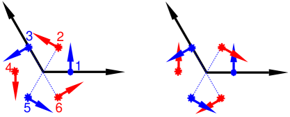
$V_{1}$ $W_{1}$

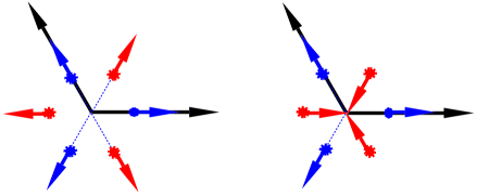
$V_{2}$ $W_{2}$

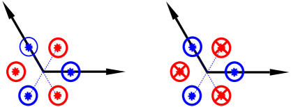
$V_{3}$ $W_{3}$

Figure 1: Schematic representation of the different magnetic orders within a unit cell. The Mn sites numbering within the unit cell are as follow $\rm Mn_{1}:(x_{\rm Mn},0,0)$, $\rm Mn_{2}:(x_{\rm Mn},x_{\rm Mn},1/2)$, $\rm Mn_{3}:(0,x_{\rm Mn},0)$, $\rm Mn_{4}:(-x_{\rm Mn},0,1/2)$, $\rm Mn_{5}:(-x_{\rm Mn},-x_{\rm Mn},0)$, $\rm Mn_{6}:(0,-x_{\rm Mn},1/2)$, where $x_{\rm Mn}\simeq 1/3$.

Associated with the AFM order, several authors reported a ferromagnetic (FM) component associated with a spin canting along the c direction. First suggested Bertaut_magn1 , and observed by Bertaut et al. Bertaut_magn2 , this FM component was later observed in the isotypic compound $\rm ScMnO_{3}$ by Xu et al. Xu_FM_Sc as well as Bieringer and Greedan Bieringer_FM_Sc . Attributed to $\rm Mn_{3}O_{4}$ impurities by Fiebig et al Fiebig_SHG , a FM component disappearing at $T_{N}$ was later observed in neutrons scattering by one of us Pailhes_FM . The controversy about the existence of such a component is thus still opened. One could argue that the weakness of the proposed canting removes most of the interest of its existence, however as we will see in the present paper the existence of a FM component has many consequences on the symmetry group of the magnetic structure as well as the interpretation of the $\rm YMnO_{3}$ properties.

Let us finally quote the existence of a giant magneto-elastic coupling observed by powder neutron diffraction at the magnetic transition Park08 ; Patnaik . Very large atomic displacements (up to 0.1Å ) are induced by the magnetic ordering without any identified change of the symmetry group. The influence of such displacements on the polarization or dielectric constant in the magnetic phase was however never reported on single crystal (such measurements exist in thin films) while this information is crucial for the assertion of the assumed magneto-electric coupling seen by domain imaging using second harmonic generation measurements Fiebig_domaines .

The present paper aims at building a coherent description for the magnetic structure of the $\rm YMnO_{3}$ compound, which will account for all the experimental observations and resolve their apparent contradictions.

II Can we get some further insight from the experiments?

II.1 Experimental details

All the measurements reported in the present work were performed on the same single crystal, grown long time ago in Groningen by G. Nénert, from the group of T. Palstra. The sample size for dielectric measurements is $\rm a=1.1\,mm$, $\rm b=1.5\,mm$ and $\rm c=0.3\,mm$. Magnetic measurements were performed with a QD MPMS-5 SQUID magnetometer. Dielectric and polarization measurements were respectively performed in a QD PPMS-14 with Agilent 4284A LCR meter and Keithley 6517A. Magnetic fields above 14 T (and up to 25 T) were achieved in the LNCMI Grenoble. The experimental setup for the dielectric constant measurements was the same as in Caen, while the LNCMI setup was used for the magnetization. Antiferromagnetic neutron diffraction peaks were measured on 4F triple axis spectrometer in Laboratoire Léon Brillouin in Saclay on the same single crystal.

II.2 The antiferromagnetic transition

We performed neutron scattering experiments on a neutron triple axis spectrometer and checked the crystal orientation and crystalline quality. The 100 magnetic peak is associated with the antiferromagnetic order parameter. On fig. 2, the temperature dependence of its amplitude is reported, showing the magnetic transition at $T_{N}=74\rm\,K$. On the same figure, we reported the ab component of the dielectric constant, $\varepsilon$, which presents an anomaly at $T_{N}$. Let us note that the c component of $\varepsilon$ does not present any anomaly at this temperature (not shown). The strong similarity, below $T_{N}$, between the temperature dependence of the antiferromagnetic order parameter, and the non linear part of $\varepsilon$, suggests that they are closely related, and thus infers the existence of a magneto-electric coupling. One should emphasize the fact that the anomaly of the dielectric constant is not a divergence as expected in the case of a linear magneto-electric coupling. This proof of a non-linear magneto-electric coupling is of utter importance as we will see in the next section.

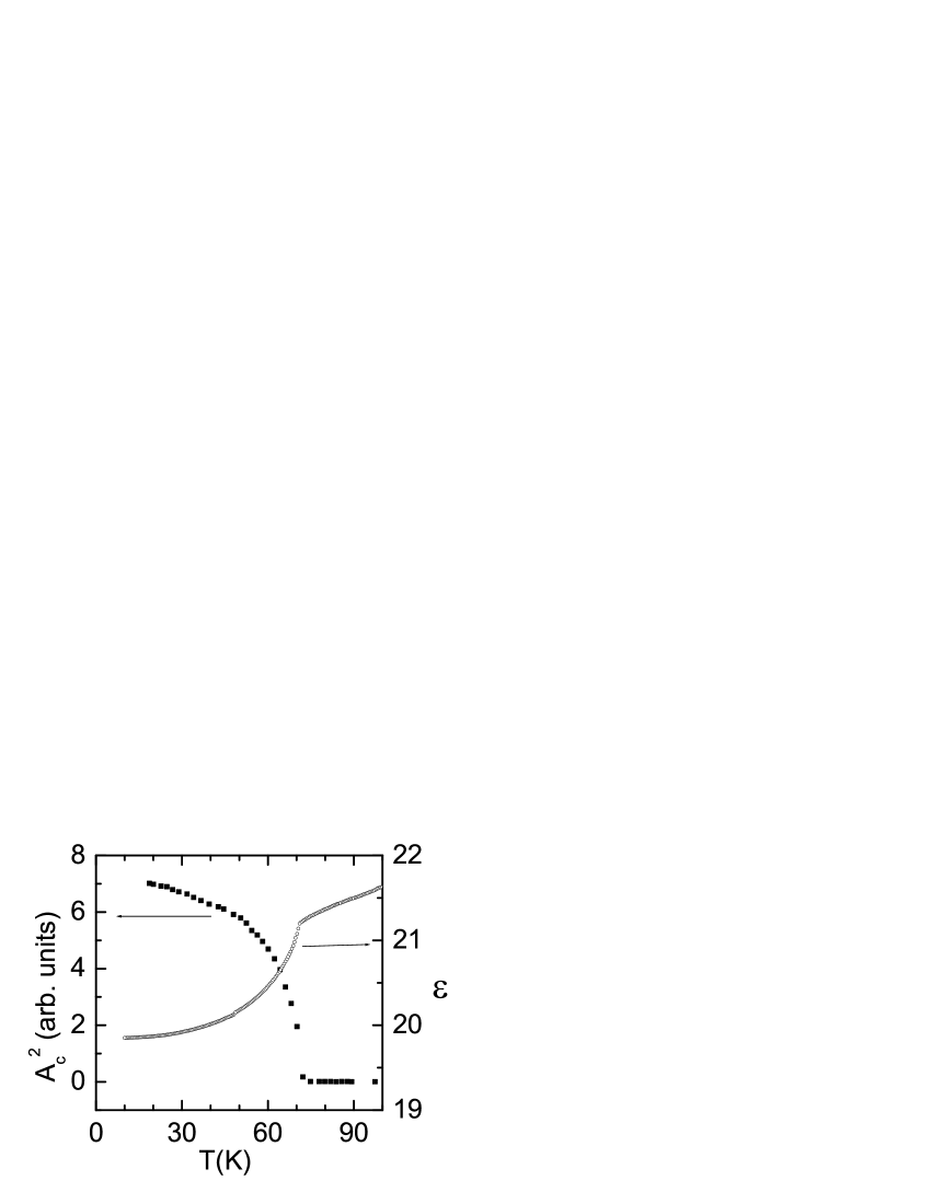
Figure 2: Temperature dependence of the 100 antiferromagnetic peak intensity (left scale) and the ab component of the dielectric constant (right scale).

II.3 The polarization and the dielectric constant

This magneto-electric coupling can also be asserted from the polarization and dielectric constant measurements in the magnetic phase.

We performed polarization measurements along the c-axis (the only one allowed by symmetry). A strong reduction of the polarization amplitude is observed below $T_{N}$ (see fig. 3) : $2\rm\,\mu C/cm^{2}$ at 30 K, to be compared with the $5.5\rm\,\mu C/cm^{2}$ measured at room temperature Kim_pol .

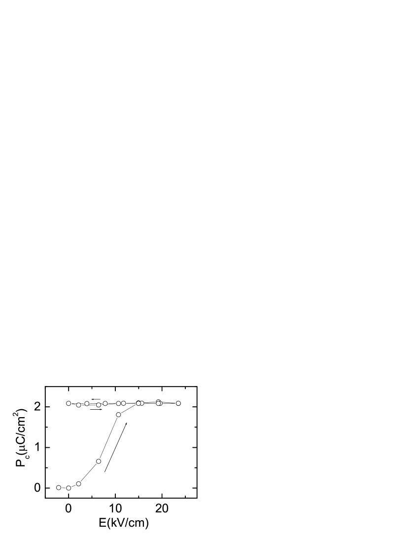
Figure 3: Polarization cycle at 30 K after cooling in a zero electric field (the polarization is very small after this procedure). The second branch of the measurement ensures that the measured current is not due to leakage (the polarization is already switched so no change is observed as the electric field is switched on again).

These polarization values are compatible with the estimated ones, obtained both as $\vec{P}=\sum_{i}q_{i}\vec{r}_{i}$ and from our first principle calculations. We computed the polarization using density functional theory and a Berry phases approach at the atomic structures given in reference Park08, at 10K and 300K. The calculations were performed with the B1PW hybrid functionals that was specifically designed for the treatment of ferroelectric oxides B1PW . At 300 K we found a polarization of $5\rm\,\mu C/cm^{2}$. in full agreement with experimental values. At 10 K, the polarization is strongly reduced to $1\rm\,\mu C/cm^{2}$ to be compared with the experimental result of $2\rm\,\mu C/cm^{2}$ at 30 K.

In addition, we measured the polarization versus the magnetic field. Since this effect is expected to be very small, we used a procedure consisting in ramping many times the magnetic field from $-14\rm\,T$ to $+14\rm\,T$ and extracting the periodic signal from the raw data. One can see on $P(H)$ taken in the magnetic phase (fig. 4) an anomaly that can be associated with a meta-magnetic transition.

Figure 4: Magnetic field dependence of the polarization at 71 K.

This anomaly can also be followed on the dielectric constant, $\varepsilon$, as a function of applied field and temperature. The meta-magnetic transition phase diagram, characteristic of an antiferromagnetic compound under magnetic field, can so be built (see fig. 5).

(a)                                                         

(b)                                                         

Figure 5: (a) Magnetic field dependence of the ab dielectric constant (H is along the c axis). (b) Corresponding phase diagram (H,T).

The searched of the meta-magnetic transition is a classical method to observe the antiferromagnetism. Indeed, in usual systems, the magnetization (or magnetic susceptibility) versus magnetic field presents an anomaly at the AFM/FM transition under applied field. In $\rm YMnO_{3}$ our ability to see this transition on electric degrees of freedom (polarization and dielectric constant) clearly proves the existence of a coupling between the polarization and the magnetic order parameter, as first proposed by Huang et al. Huang .

II.4 The ferromagnetic component

As mentioned in the introduction, one of us (S. Pailhès) observed in a non-polarized neutrons scattering experiment, a Bragg peak that was associated with a ferromagnetic component Pailhes_FM . Indeed, this Bragg peak, at $\vec{q}=(2,-1,1)$, can neither be associated with the antiferromagnetic order within the (a,b) plane, nor with the nuclear extinction rules, since for the $P6_{3}cm$ symmetry group imposes $2l=0$. In addition it disappears at $T_{N}$, as expected from a canted AFM order. One objection can however be made against this interpretation. The existence of two $\rm MnO_{3}$ layers per unit cell (respectively at $z=0$ and $z=1/2$) , forbids to rule out the possibility of an antiferromagnetic coupling between the c components of the canted magnetic moments of each layer ($W_{3}$ versus $V_{3}$ order of figure 1).

We thus performed precise magnetic measurements on a SQUID magnetometer at low magnetic field, and we did observe a small FM component (see fig. 6). The sample was cooled down from 100 K (still above $T_{N}$) to 10 K either under an applied magnetic field along the c axis of the crystal (Field Cooled =FC) or without any field (Zero Field Cooled = ZFC). After cooling, the magnetization was always measured ramping the temperature up under the applied field. This procedure, assuming that the applied field is too small to reverse the magnetization, clearly evidenced the existence of a ferromagnetic component along the c axis (see fig. 6). The applied magnetic field is 0.05 T.

Figure 6: Ferromagnetic component M as a function of temperature. In the inset, the raw data in field cooled (FC) and zero field cooled (ZFC) modes. The sample mass is 31.5 mg.

III Can we build a theoretical description compatible with the above experimental facts?

Let us summarize the facts we learned from experiments.

• $\rm YMnO_{3}$ exhibits a magneto-electric coupling between the AFM and the FE orders.

• This magneto-electric coupling is non linear. The immediate consequence of this is that the AFM order parameter cannot be in the same irreducible representation than the FE order parameter, that is the polarization. The latter being in the totally symmetric irreducible representation : $\Gamma_{1}$, the AFM order cannot belong to the $\Gamma_{1}$ irreducible representation of the magnetic group. Assuming that the magnetic order found by Bertaut Bertaut_magn1 ; Bertaut_magn2 and Muñoz Munoz_neutrons is correct, it means that the magnetic group is not $P6_{3}cm$ as assumed by these authors. See $V_{1}$ of fig. 1 for a picture of this order.

• There is a weak FM component along the c axis.

• Even if essentially quenched by the crystal field splitting of the Mn $3d$ orbitals, the spin-orbit coupling and thus the Dzyaloshinskii–Moriya (DM) interaction always exists provided it is symmetry allowed. This is the case with the AFM magnetic order $V_{1}$ found in neutrons scattering, since the spins vorticity is non nil. The DM interaction should thus induces a FM component (even if small) along the c direction.

• Finally the AFM and FM order parameters are not linearly coupled. Indeed, they present different behaviors around the transition (see figure 7 of ref. Pailhes_FM, or figures 2 and 6 of the present paper).

According to the above analysis the $P6_{3}cm$ group cannot be the system magnetic group. Can we find a magnetic subgroup of the crystallographic group $P6_{3}cm$ compatible with all the above experimental requirements? The following symmetry group analysis tells us that only one magnetic group is compatible with (i) the $V_{1}$ AFM order, (ii) the fact that this order is not in the $\Gamma_{1}$ irreducible representation and (iii) the existence of a FM component along the c direction. This group is the $P6_{3}^{\prime}$ magnetic group. Indeed, we first examined the magnetic groups associated with the $P6_{3}cm$ crystallographic group, that is

$P6_{3}cm$ :

discarded since the AFM order $V_{1}$ belongs to $\Gamma_{1}$ and the FM component $V_{3}$ is not allowed (does not belong to the same representation as $V_{1}$);

$P6_{3}^{\prime}c^{\prime}m$ :

discarded since $V_{1}$ and $V_{3}$ do not belong to the same representation (FM component not allowed);

$P6_{3}^{\prime}cm^{\prime}$ :

discarded since the FM component is not allowed;

$P6_{3}c^{\prime}m^{\prime}$ :

discarded since the FM component is not allowed.

Since none of them is compatible with the experimental requirements we looked further in their subgroups and thus abandoned the mirror planes.

The $\bf P6_{3}$ group

was discarded since $V_{1}$ belongs to $\Gamma_{1}$, which is incompatible with the absence of a linear magneto-electric coupling.

Finally the $\bf P6_{3}^{\prime}$ group

is the only group compatible with all the requirements.

Let us remember that the $P6_{3}^{\prime}$ magnetic group was strongly suggested by Brown and Chatterji Tapan from the polarimetric study of neutron diffraction. In fact, they were the first to suggest that the mirror planes are incompatible with the $\rm YMnO_{3}$ magnetic group.

Let us now see whether we can account for all the experimental results in a Landau analysis. We established that the magnetic transition should be a transition between the paramagnetic (PM) phase belonging to the $P6_{3}cm$ group, and the antiferromagnetic (AFM) phase belonging to the $P6_{3}^{\prime}$ group. In the $P6_{3}^{\prime}$ group the $\Gamma_{4}$ irreducible representation, to whom both the AFM ($V_{1}$) and the FM ($V_{3}$) order parameters belong, is three times represented, namely by the $V_{1}$, $V_{2}$ and $V_{3}$. The Landau theory must thus involve all three magnetic order parameters in addition to the change in the ferroelectric polarization. $V_{1}$ and $V_{2}$ are easily represented by the toroidal ($\vec{A}$) and divergence ($B$) components of the in-plane spins component, while $V_{3}$ is the out of plane component associated with the magnetization ($\vec{M}$). For each unit cell one can thus define

$$\vec{A} = \frac{1}{6r}\sum_{i}\vec{r}_{i}\wedge\vec{S}_{i}=\frac{1}{6r}\sum_{i}\vec{r}_{i}\wedge\vec{S}_{ab,i}$$

$$B = \frac{1}{6r}\sum_{i}\vec{r}_{i}\cdot\vec{S}_{i}=\frac{1}{6r}\sum_{i}\vec{r}_{i}\cdot\vec{S}_{ab,i}$$

$$\vec{M} = \frac{1}{6}\sum_{i}\vec{S}_{i}=\frac{1}{6}\sum_{i}\vec{S}_{c,i}$$

where the summations over $i$ run over the six Mn atoms of the unit cell ; the $\vec{r}_{i}$ refer to the in plane components of the Mn atoms position vectors (note that $\sum_{i}\vec{r}_{i}=\vec{0}$ and $\forall i\,|\vec{r}_{i}|=r$) ; the $\vec{S}_{i}$ are the Mn atomic spins ($\vec{S}_{i}=\vec{S}_{ab,i}+\vec{S}_{c,i}$ where $\vec{S}_{ab,i}$ is the in-plane component of the Mn spins and $\vec{S}_{c,i}$ is the c axis component).

$\vec{A}$ and $\vec{M}$ are vectors along the c direction while $B$ is a scalar. Let use write $A=S_{ab}\cos{\varphi}$ and $B=S_{ab}\sin{\varphi}$ and point out that the intensity of the 100 AFM magnetic peak (fig. 2) is proportional to ${S_{ab}}^{2}$ whatever the angle $\varphi$. In the paramagnetic state, i.e. for $T>T_{N}$, $S_{ab}=0$, but the polarization $P$ is not zero. This is one of the important issue of this compound. $\vec{P}$ is not a driving order parameter for the magnetic transition ; however, since its value presents a singularity at $T_{N}$, it is a secondary order parameter. Its contribution should thus be taken into account in the Landau free energy and can only contain even powers of $P$, as imposed by the higher temperature paraelectric to ferroelectric transition. The free energy can thus be expressed up to the power 4 of the order parameters

$$F = \overbrace{\alpha_{2}(T-T_{N})(A^{2}+B^{2})+\alpha_{4}(A^{2}+B^{2})^{2}}^{\text{AFM energy}}$$

$$\overbrace{-\beta_{2}(P^{2}-{P_{0}}^{2})+\beta_{4}(P^{4}-{P_{0}}^{4})}^{\text{change in the FE energy}}$$

$$\overbrace{+\gamma_{2}M^{2}+\gamma_{4}M^{4}}^{\text{FM energy}}$$

$$\overbrace{+c_{4}(A^{2}+B^{2})(P^{2}-{P_{0}}^{2})}^{\text{AFM/FE coupling}}$$

$$\overbrace{+d_{4}M^{2}(P^{2}-{P_{0}}^{2})}^{\text{FM/FE coupling}}$$

$$\overbrace{+e_{4}(A^{2}+B^{2})M^{2}}^{\text{AFM/FM coupling}}$$

$$\overbrace{+z_{4}(P^{2}-{P_{0}}^{2})\vec{A}\cdot\vec{M}}^{\text{Dzyaloshinskii–Moriya interaction}}$$

where $\alpha_{2}$, $\alpha_{4}$, $\beta_{2}$, $\beta_{4}$, $\gamma_{2}$, $c_{4}$, $d_{4}$, $e_{4}$, $z_{4}$ are the temperature independent Landau expansion coefficients. If one notes $t=T_{N}-T$, and $\vec{\delta P}=\vec{P}-\vec{P}_{0}$ the gradient of the free energy writes as

$$\frac{\partial F}{\partial S_{ab}} = S_{ab}\left[-2\alpha_{2}\,t+4\alpha_{4}\,{S_{ab}}^{2}+2c_{4}\delta\!P\,(2P_{0}+\delta\!P)\right.$$

$$\left.+2e_{4}M^{2}\right]+z_{4}\,\cos{\varphi}\,M\,\delta\!P\,(2P_{0}+\delta\!P)=0$$

$$\frac{\partial F}{\partial\delta\!P} = (P_{0}+\delta\!P)\left[-2\beta_{2}+4\beta_{4}\,({P_{0}}^{2}+2{P_{0}}\delta\!P+{\delta\!P}^{2})\right.$$

$$\left.+2c_{4}\,{S_{ab}}^{2}+2d_{4}\,M^{2}\quad+2z_{4}\,S_{ab}\,M\,\cos{\varphi}\right]=0$$

$$\frac{\partial F}{\partial\varphi} = z_{4}\,S_{ab}\,M\,\sin{\varphi}\,\delta\!P\,(2P_{0}+\delta\!P)=0$$

$$\frac{\partial F}{\partial M} = M\,\left[2\gamma_{2}+4\gamma_{4}M^{2}+2d_{4}\,\delta\!P\,(2P_{0}+\delta\!P)+2e_{4}{S_{ab}}^{2}\right]$$

$$+z_{4}\,S_{ab}\,\cos{\varphi}\,\delta\!P\,(2P_{0}+\delta\!P)=0$$

From the experimental results we know that $M\ll{S_{ab}}^{2}$ and $\delta\!P$. We thus expect that if $S_{ab}\propto t^{\nu}$, $\delta\!P\propto t^{\mu}$ and $M\propto t^{\eta}$, we will have in the vicinity of the transition $\eta>\mu$ and $\eta>2\nu$. In an order by order expansion of the free energy gradient as a function of $t$, one can thus suppose either that $\eta>\nu+1$ ($M\ll S_{ab}t$) or that $\eta\sim\nu+1$ ($M\sim S_{ab}t$). It is easy to show that the first hypothesis leads to a contradiction. Let us thus assume that $M\sim S_{ab}t$. One gets at the zeroth order in $t$

$$\frac{\partial F}{\partial\delta\!P}=P_{0}\left[-2\beta_{2}+4\beta_{4}\,{P_{0}}^{2}\right]=0 \quad\Leftrightarrow\quad P_{0}^{2}=\frac{\beta_{2}}{2\beta_{4}}$$

and at the following order

$$\left\{\begin{array}[c]{lcl}\frac{\partial F}{\partial S_{ab}}&:&S_{ab}\left[-2\alpha_{2}\,t+4\alpha_{4}\,{S_{ab}}^{2}\ +4c_{4}P_{0}\delta\!P\right]=0\\[4.30554pt] \frac{\partial F}{\partial\delta\!P}&:&8\beta_{4}\,{P_{0}}^{2}\delta\!P+2c_{4}P_{0}\,{S_{ab}}^{2}=0\end{array}\right.$$

$$\Leftrightarrow \left\{\begin{array}[c]{lcl}{S_{ab}}^{2}&=&\frac{\alpha_{2}\,\beta_{2}}{2\alpha_{4}\,\beta_{2}-{c_{4}}^{2}{P_{0}}^{2}}\,t\\[4.30554pt] \delta\!P&=&-\frac{\alpha_{2}\,c_{4}P_{0}}{4\alpha_{4}\,\beta_{2}-2{c_{4}}^{2}{P_{0}}^{2}}\,t\end{array}\right.$$

$$\frac{\partial F}{\partial\varphi} :\quad 2z_{4}P_{0}\,S_{ab}\,M\,\sin{\varphi}\,\delta\!P=0\quad\Leftrightarrow\quad\sin{\varphi}=0$$

$$\frac{\partial F}{\partial M} :\quad 2\gamma_{2}M+2z_{4}P_{0}\,S_{ab}\,\cos{\varphi}\,\delta\!P=0$$

$$\Leftrightarrow M=\frac{{\alpha_{2}}^{3/2}\,{\beta_{2}}^{1/2}c_{4}z_{4}{P_{0}}^{2}}{2\gamma_{2}\,(2\alpha_{4}\,\beta_{2}-{c_{4}}^{2}{P_{0}}^{2})^{3/2}}\,\cos{\varphi}\,t^{3/2}$$

We thus retrieve the $V_{1}$ order for the AFM spins arrangement ($\sin{\varphi}=0$)  ; the decrease in the polarization amplitude under the Néel transition ($\delta P<0$), the fact that the FM order parameter is much weaker than both the AFM one and the change in the polarization ($\nu=1/2$, $\mu=1$, $\eta=3/2$), and finally the fact the FM and AFM order parameters are not linearly related at $T_{N}$. The polarization and the square of the AFM order parameter are predicted to vary linearly in $t$ at the magnetic transition, as a classical second order phase transition. In fact, as it is for most magnetic phase transitions, higher order terms in the free energy make the temperature dependence over a large scale of temperature different from the mean field prediction. Here for example, the best fit for ${S_{ab}}^{2}$ is a power law in $t^{1/3}$ (not shown in fig. 2).

Coming back to the anomaly of the dielectric constant at $T_{N}$ and using the second derivative of $F$ with respect to $P$, one gets in the first order in $t$

$$\frac{1}{\chi_{e}} = \frac{\partial^{2}F}{\partial{\delta\!P}^{2}}=4\beta_{2}-6\,c_{4}\,S^{2}+2c_{4}\,S^{2}=4(\beta_{2}-c_{4}\,S^{2})$$

$$\text{and}\quad\varepsilon = 1+\chi_{e}$$

$$= 1+\frac{1}{4\beta_{2}}+\frac{c_{4}}{4{\beta_{2}}^{2}}\,S^{2}$$

Comparing the above expression with the experimental data of fig. 2, the Landau analysis correctly predicts the critical shape of $\varepsilon$ versus the AFM order parameter ${S_{ab}}^{2}$.

As a first conclusion one can state that the above Landau analysis seems in perfect agreement with all the experimental data. The most important consequence of it is that one cannot switch the direction of any of the magnetic orders — clockwise vs counter clockwise rotation of the antiferromagnetic order (sign of $A$) or direction of the magnetization (sign of $M$) — by switching $P$. Indeed, one has $P=P_{0}\left(1-\frac{c_{4}}{4\beta_{4}}\,A^{2}\right)$, and $M=-\frac{z_{4}}{\gamma_{2}}\,A\,P_{0}\delta\!P$ thus a change in the sign of $P$ will leave the sign of both $A$ and $M$ unchanged. On the contrary, $A$ and $M$ are switched simultaneously.

IV Are there other options?

If one supposes that the weak FM component is artefactual, then there are three different groups compatible with the $V_{1}$ AFM order and the absence of a linear magneto-electric coupling, that is : $P6_{3}^{\prime}c^{\prime}m$, $P6_{3}^{\prime}cm^{\prime}$ and $P6_{3}c^{\prime}m^{\prime}$. In such a case however it is difficult to explain why the $\vec{D}_{ij}.(\vec{S}_{i}\wedge\vec{S}_{j})$ Dzyaloshinskii-Moriya interaction does not yield a FM component along the $\bf c$ direction. Giving up the FM component thus means giving up the $V_{1}$ ordering for the AFM order.

Is there another AFM order compatible with the neutrons scattering experiments? Following Bertaut Bertaut_magn3 and Muñoz Munoz_neutrons , there is indeed another AFM order possibly compatible with the neutrons diffraction data, even if with a significantly worse agreement factor than $V_{1}$ ($R_{\text{MAG}}=10.8\%$ instead of $7.6\%$ Munoz_neutrons ). This order is pictured as $W_{2}$ in fig. 1. It is compatible with a non-linear magneto-electric coupling in the $P6_{3}cm$, $P6_{3}^{\prime}c^{\prime}m$, $P6_{3}c^{\prime}m^{\prime}$ and $P6_{3}$ magnetic groups. In the $P6_{3}cm$, $P6_{3}^{\prime}c^{\prime}m$ and $P6_{3}c^{\prime}m^{\prime}$ groups it is associated in its irreducible representation with the $W_{3}$ order, while in the $P6_{3}$ magnetic groups both the $W_{1}$ and $W_{3}$ orders belong to the representation of $W_{2}$. At this point let us note that the $W_{3}$ AFM order is compatible with the $(2,-1,1)$ peak observed by Pailhès et al Pailhes_FM in neutrons scattering.

IV.1 What Landau’s theory tells us ?

In the $P6_{3}cm$, $P6_{3}^{\prime}c^{\prime}m$ and $P6_{3}c^{\prime}m^{\prime}$ groups the Landau analysis yields

$$F = \alpha_{2}(T-T_{N})B^{\prime 2}+\alpha_{4}B^{\prime 4}\quad+\quad\gamma_{2}M^{\prime 2}+\gamma_{4}M^{\prime 4}$$

$$-\beta_{2}(P^{2}-{P_{0}}^{2})+\beta_{4}(P^{4}-{P_{0}}^{4})$$

$$+c_{4}B^{\prime 2}(P^{2}-{P_{0}}^{2})+d_{4}M^{\prime 2}(P^{2}-{P_{0}}^{2})+e_{4}B^{\prime 2}M^{\prime 2}$$

where $B^{\prime}$ and $M^{\prime}$ are the order parameters respectively associated with $W_{2}$ and $W_{3}$.

$$B^{\prime} = \frac{1}{6r}\sum_{i}(-1)^{i}\vec{r}_{i}\cdot\vec{S}_{i}=\frac{1}{6r}\sum_{i}(-1)^{i}\vec{r}_{i}\cdot\vec{S}_{i}^{a,b}$$

$$\vec{M}^{\prime} = \frac{1}{6}\sum_{i}(-1)^{i}\vec{S}_{i}=\frac{1}{6}\sum_{i}(-1)^{i}\vec{S}_{c,i}$$

$$\frac{\partial F}{\partial S_{ab}} = S_{ab}\left[-2\alpha_{2}\,t+4\alpha_{4}\,{S_{ab}}^{2}+2c_{4}\delta\!P\,(2P_{0}+\delta\!P)\right.$$

$$\left.+2e_{4}M^{\prime 2}\right]=0$$

$$\frac{\partial F}{\partial\delta\!P} = (P_{0}+\delta\!P)\left[-2\beta_{2}+4\beta_{4}\,({P_{0}}^{2}+2{P_{0}}\delta\!P+{\delta\!P}^{2})\right.$$

$$\left.+2c_{4}\,{S_{ab}}^{2}+2d_{4}\,M^{\prime 2}\right]=0$$

$$\frac{\partial F}{\partial M^{\prime}} = M^{\prime}\,\left[2\gamma_{2}+4\gamma_{4}M^{\prime 2}+2d_{4}\,\delta\!P\,(2P_{0}+\delta\!P)\right.$$

$$\left.+2e_{4}{S_{ab}}^{2}\right]=0$$

These equations give

$$P_{0}^{2} = \frac{\beta_{2}}{2\beta_{4}}$$

$${S_{ab}}^{2}=\frac{\alpha_{2}\,\beta_{2}}{2\alpha_{4}\,\beta_{2}-{c_{4}}^{2}{P_{0}}^{2}}\,t \delta\!P=-\frac{\alpha_{2}\,c_{4}P_{0}}{4\alpha_{4}\,\beta_{2}-2{c_{4}}^{2}{P_{0}}^{2}}\,t$$ and

$$\text{and finally}\qquad M^{\prime} = 0$$

One sees that these results are equivalent to the previous derivation as far as $S_{ab}$ and $P$ are concerned. However, if $M^{\prime}=0$ is coherent with the neutrons scattering results of ref. Munoz_neutrons , it is not compatible with the existence of the $(2,-1,1)$ peak observed by Pailhès et al Pailhes_FM . Indeed, in this representation the $(2,-1,1)$ peak measures the intensity of the order parameter $M^{\prime}$.

IV.2 What about the second harmonic generation experiments?

The second harmonic spectra are due to $d$–$d$ electronic transitions within the $\rm Mn^{3+}$ ions (see figure 7). The non linear succeptibility is dominated by the term starting from the atomic ground state ($S=2$) and can be written as

$$\epsilon_{0}\;\chi_{\alpha\beta\gamma} = \sum_{m,k}\frac{\langle 0|\hat{P}_{\alpha}|m\rangle\langle m|\hat{P}_{\beta}|k\rangle\langle k|\hat{P}_{\gamma}|0\rangle}{(\hbar\omega_{mi}-2\hbar\omega)(\hbar\omega_{ki}-\hbar\omega)}$$

where $|0\rangle$ is the $\rm Mn^{3+}$ atomic ground state ; $|k\rangle$ and $|m\rangle$ span the $d$–$d$ $\rm Mn^{3+}$ excited states, $\hbar\omega_{ki}$ and $\hbar\omega_{mi}$ being their excitation energies ; $\hat{P}_{\alpha}$ are the dipolar moment operators along the $\alpha$ direction.

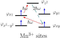
Figure 7: Example of the two photons absorption (in dotted red) and one photon emission (in dashed blue-grey) responsible for the second harmonic generation.

We thus evaluated both the in-plane, $\epsilon_{0}\;\chi_{xxx}$ and $\epsilon_{0}\;\chi_{yyy}$, and the out-of-plane components, $\epsilon_{0}\;\chi_{zxx},\,\epsilon_{0}\;\chi_{zyy}$, for the different magnetic groups and orders discussed in this paper. The detailed calculations can be found in Appendix.

For the magnetic groups associated with the $P6_{3}cm$ space group we found

$$\epsilon_{0}\,\chi_{xxx}(z\!=\!0) = \epsilon_{0}\,\chi_{xxx}^{0}(z\!=\!0)$$

$$+\left[\frac{A}{\varepsilon_{z^{2}}-\varepsilon_{x^{2}-y^{2}}-2\hbar\omega}+\frac{A^{\prime}}{\varepsilon_{z^{2}}-\varepsilon_{xy}-2\hbar\omega}\right]\langle S_{x}\rangle_{{\rm Mn}_{1}}$$

$$+\left[\frac{B}{\varepsilon_{z^{2}}-\varepsilon_{x^{2}-y^{2}}-2\hbar\omega}+\frac{B^{\prime}}{\varepsilon_{z^{2}}-\varepsilon_{xy}-2\hbar\omega}\right]\langle S_{x}\rangle_{{\rm Mn}_{1}}^{2}$$

$$\epsilon_{0}\,\chi_{yyy}(z\!=\!0) = 0$$

$$\epsilon_{0}\,\chi_{zxx}(z\!=\!0) = \epsilon_{0}\,\chi_{zxx}^{0}(z\!=\!0)+\frac{C}{\varepsilon_{z^{2}}-\varepsilon_{x^{2}-y^{2}}-2\hbar\omega}\langle S_{x}\rangle_{{\rm Mn}_{1}}$$

$$+\frac{D}{\varepsilon_{z^{2}}-\varepsilon_{x^{2}-y^{2}}-2\hbar\omega}\langle S_{x}\rangle_{{\rm Mn}_{1}}^{2}+\frac{E}{\varepsilon_{z^{2}}-\varepsilon_{x^{2}-y^{2}}-2\hbar\omega}\langle S_{x}\rangle_{{\rm Mn}_{1}}^{3}$$

and similarly for the $z\!=\!1/2$ layer ($\rm Mn_{1}$ being replaced by $\rm Mn_{4}$). $\chi_{xxx}^{0}(z\!=\!0)$ is the spin independent (FE) tensor, $\varepsilon_{i}$ the energy of the iron orbital $\varphi_{i}\simeq 3d_{i}$ and $\langle S_{\alpha}\rangle_{{\rm Mn}_{i}}$ the $\alpha$ component of the spin of the $\rm Mn_{i}$ atom. $x,y,z$ are orthogonal axes, $x$ being along the crystallographic $a$ direction and $k$ along the crystallographic $c$ direction.

From these results one can derive the following conclusions.

• Within the symmetry rules associated with a $P6_{3}cm$ crystal group the second harmonic signal can only be sensitive to magnetic orders in which $\langle S_{x}\rangle_{{\rm Mn}_{1}}\neq 0$ and/or $\langle S_{x}\rangle_{{\rm Mn}_{4}}\neq 0$.

• The experimental data Frohlich_SHG that sees a magnetic contribution to the in-plane component of $\chi$ are thus incompatible with the $V_{1}$ magnetic order as previously shown by Iizuka-Sakano Ii_SHG and coherently with our previous analysis.

• We showed that the only possible magnetic order compatible with a $P6_{3}cm$ crystal group is $W_{2}$ in which $\langle S_{x}\rangle_{{\rm Mn}_{1}}=\langle S_{x}\rangle_{{\rm Mn}_{4}}\neq 0$. According to equations The magnetic groups associated with the $P6_{3}cm$ crystal group this order predicts a magnetic contribution to the in-plane component of $\chi$, but also to the out-of-plane one $\chi_{zxx}=\chi_{zyy}$. While the first one is in agreement with the experimental findings, no magnetic signal was found in the out-of-plane SHG signal.

• The $P6_{3}cm$ crystal group and associated magnetic groups are thus not only incompatible with the existence of a FM component and the $(2,-1,1)$ peak observed by neutrons scattering but also with the SHG experimental data.

Let us thus go back to the $P6_{3}^{\prime}$ magnetic group and remember that, up to now, this group was found compatible with all experimental facts. The calculation yields the following form for the $\chi$ components (only the contributions associated with the $V_{1}$ and $V_{3}$ magnetic orders compatible with the $P6_{3}^{\prime}$ magnetic group are retained)

$$\epsilon_{0}\,\chi_{xxx}(z=0) = \epsilon_{0}\,\chi_{xxx}^{0}(z=0)$$

$$+{\bf i}\left[\frac{A}{\varepsilon_{z^{2}}-\varepsilon_{x^{2}-y^{2}}-2\hbar\omega}+\frac{A^{\prime}}{\varepsilon_{z^{2}}-\varepsilon_{xy}-2\hbar\omega}\right]\langle S_{y}\rangle_{\rm Mn_{1}}\langle S_{z}\rangle_{\rm Mn_{1}}$$

$$+\left[\frac{B}{\varepsilon_{z^{2}}-\varepsilon_{x^{2}-y^{2}}-2\hbar\omega}+\frac{B^{\prime}}{\varepsilon_{z^{2}}-\varepsilon_{xy}-2\hbar\omega}\right]\langle S_{y}\rangle_{\rm Mn_{1}}^{2}$$

$$\epsilon_{0}\,\chi_{yyy}(z=0) = \epsilon_{0}\,\chi_{yyy}^{0}(z=0)$$

$$+\left[\frac{C}{\varepsilon_{z^{2}}-\varepsilon_{x^{2}-y^{2}}-2\hbar\omega}+\frac{C^{\prime}}{\varepsilon_{z^{2}}-\varepsilon_{xy}-2\hbar\omega}\right]\langle S_{y}\rangle_{\rm Mn_{1}}$$

$$+{\bf i}\,\left[\left(\frac{D}{\varepsilon_{z^{2}}-\varepsilon_{x^{2}-y^{2}}-2\hbar\omega}+\frac{D^{\prime}}{\varepsilon_{z^{2}}-\varepsilon_{xy}-2\hbar\omega}\right)\langle S_{y}\rangle_{\rm Mn_{1}}^{2}\right.$$

$$\left.+\left(\frac{E}{\varepsilon_{z^{2}}-\varepsilon_{x^{2}-y^{2}}-2\hbar\omega}+\frac{E^{\prime}}{\varepsilon_{z^{2}}-\varepsilon_{xy}-2\hbar\omega}\right)\right]\langle S_{z}\rangle_{\rm Mn_{1}}$$

$$\epsilon_{0}\chi_{zxx}(z=0) = \epsilon_{0}\chi_{zyy}(z=0)\;=\;\epsilon_{0}\chi_{zxx}^{0}$$

$$\;+\;\left[\frac{A}{\varepsilon_{z^{2}}-\varepsilon_{x^{2}-y^{2}}-2\hbar\omega}+\frac{A^{\prime}}{\varepsilon_{z^{2}}-\varepsilon_{xy}-2\hbar\omega}\right]\langle S_{y}\rangle_{\rm Mn_{1}}^{2}$$

Let us remember that the $V_{1}$ and $V_{3}$ orders cannot be reversed independently ($\langle S_{y}\rangle_{\rm Mn_{1}}\langle S_{z}\rangle_{\rm Mn_{1}}>0$ whatever the magnetic domain), and that $\langle S_{y}\rangle_{\rm Mn_{1}}=-\langle S_{y}\rangle_{\rm Mn_{4}}$, $\langle S_{z}\rangle_{\rm Mn_{1}}=\langle S_{z}\rangle_{\rm Mn_{4}}$. One thus sees immediately that $\chi_{xxx}$ and $\chi_{zxx}$ depend only on $\langle S_{y}\rangle_{\rm Mn_{1}}^{2}$ and should thus be insensitive to the magnetic domains. On the contrary, $\chi_{yyy}$ depend on $\langle S_{z}\rangle_{\rm Mn_{1}}$ and should thus exhibit a sensitivity to the magnetic domains at two different frequencies ; namely $2\hbar\omega=\varepsilon_{z^{2}}-\varepsilon_{xy}$ and $2\hbar\omega=\varepsilon_{z^{2}}-\varepsilon_{x^{2}-y^{2}}$, differing by $\Delta E^{\prime}$. Those results are in full agreement with the experimental data reported on reference Frohlich_SHG, .

V Conclusion

In the present paper we showed from joined experimental evidences and theoretical analysis that the AFM transition in $\rm YMnO_{3}$ is associated with three order parameters, namely the AFM one (primary order parameter), the extra-component of the polarization along c and the ferromagnetic component along the c axis induced by the Dzyaloshinskii-Moriya interaction (secondary order parameters). Moreover the analysis of the magnetic transition showed the absence of linear coupling between them and thus a hierarchy. Taking into account the different experimental observations (magnetic and transport macroscopic measurements, neutrons scattering data, optical second harmonic responses), as well as the presence of the DM coupling, it appears that the $P6_{3}^{\prime}$ magnetic group is the only possible one. In the past, many publications tried to address this question with different conclusions, but all of them present unsolved questions or problems we tried to address in the present work. For example, the importance of a ferromagnetic component was underlined by Bertaut, but corresponds in his samples to a parasitic phase ; some authors have discarded magnetic groups, assuming that the magnetic order should belong to the $\Gamma_{1}$ irreducible representation of the symmetry group, and so forgetting that despite being by far the most frequent, this is not the only possibility and any of the group representation is valid for the wave function. In fact, the absence of a divergence in the dielectric constant at the phase transition implies that the magneto-electric coupling is not linear, and thus that the polarization and the AFM order cannot belong to the same irreducible representation. The polarization being of $\Gamma_{1}$ symmetry, the magnetic order cannot belong to the totally symmetric representation $\Gamma_{1}$. This, in addition to the presence of the small ferromagnetic component, implies that the only possible group is here $P6_{3}^{\prime}$. In this group, a change in the sign of the polarization, P, will let both the weak magnetization, M, and the AFM order parameter, A, unchanged. On the contrary, A and M will be switched simultaneously. For possible applications, this type of multiferroic cannot be used to switch the magnetization with an electric field, but rather to switch antiferromagnetism with an intense magnetic field, providing memories which are only little sensitive to magnetic fields.

Appendix

General considerations

In the following appendix the SHG equations are expressed in term of an orthogonal $x,y,z$ set of axes. The $x$ axis is along the $a$ direction, that is associated with one of the O–Mn bonds in the $z=0$ layer (O is the $(0,0,z\simeq 0)$ in-plane oxygen), the $y$ axis its in-plane orthogonal and the $z$ axis is along the $c$ direction.

The three-fold rotation axis is present in any of the groups proposed in this paper. We can thus use it in order to express the $\chi_{\alpha\beta\gamma}$ tensor for the $z=0$ layers as a function of its value for the $\rm Mn_{1}$ ion (see fig. 1 for the ions labeling), and for the $z=1/2$ layer as a function of its value for the $\rm Mn_{4}$ ion. One gets easily

$$\chi_{xxx}(z=0) = \frac{3}{4}\left(\chi_{xxx}({\rm Mn}_{1})-\sum\chi_{xyy}({\rm Mn}_{1})\right)$$

$$\chi_{zxx}(z=0) = \frac{3}{2}\left(\chi_{xxz}({\rm Mn}_{1})+\chi_{yyz}({\rm Mn}_{1})\right)$$

$$\chi_{xzz}(z=0) = 0$$

and similarly for $z=1/2$ with $\rm Mn_{4}$ or for $\chi_{yyy},\chi_{zyy},\chi_{yzz}$. The summation $\sum\chi_{xyy}$ must be intended as a sum over all similar terms, that is $\sum\chi_{xyy}=\chi_{xyy}+\chi_{yxy}+\chi_{yyx}$.

Starting from the high temperature phase, we will proceed in perturbation (up to the first order in the wave functions, second order in energy) to include the different symmetry breaking at the FE and AFM transitions, as well as the spin-orbit interaction. In the $P6_{3}/mmc$ high temperature group, the Mn ions are located on sites of $D_{3h}$ symmetry and one gets the following $3d$ zeroth order orbitals (associated with a nil non linear succeptibility tensor)

$$\varphi_{z^{2}} = d_{z^{2}}$$

$$\varphi_{xz} = d_{xz}$$

$$\varphi_{yz} = d_{yz}$$

$$\varphi_{x^{2}-y^{2}} = cd_{x^{2}-y^{2}}+c^{\prime}p_{x}$$

$$\varphi_{xy} = cd_{xy}+c^{\prime}p_{y}$$

At this point let us notice that the $d_{x^{2}-y^{2}}$ and $p_{x}$ (as well as the $d_{xy}$ and $p_{y}$) Mn orbitals belong to the same irreducible representation and are thus hybridized through the metal-ligand interactions.

The magnetic groups associated with the $P6_{3}cm$ crystal group

Going through the FE transition toward the $P6_{3}cm$ group, the Mn ions goes from a $D_{3h}$ site to a $C_{s}$ symmetry site, thus the degeneracies between $\varphi_{xz}\,/\,\varphi_{yz}$ and the $\varphi_{x^{2}-y^{2}}\,/\,\varphi_{xy}$ orbitals are lifted by respectively $\delta E$ and $\delta E^{\prime}$. At the first order of perturbation in this symmetry breaking and in the spin orbit coupling, one gets the following orbitals

$$\varphi_{z^{2}} = d_{z^{2}}+\varsigma p_{z}+\mu d_{xz}+\nu(cd_{x^{2}-y^{2}}+c^{\prime}p_{x})$$

$$+\frac{\sqrt{3}\aleph}{\Delta\varepsilon_{2}}\left[\langle S_{x}\rangle d_{xz}+\langle S_{y}\rangle d_{yz}\right]$$

$$\varphi_{xz} = d_{xz}+\lambda(cd_{x^{2}-y^{2}}+c^{\prime}p_{x})-\mu d_{z^{2}}+\varsigma^{\prime}p_{z}$$

$$-\frac{\sqrt{3}\aleph}{\Delta\varepsilon_{2}}\langle S_{x}\rangle d_{z^{2}}+i\frac{\aleph}{\delta E}\langle S_{z}\rangle d_{yz}$$

$$+\frac{c\aleph}{\Delta\varepsilon_{1}}\left[\langle S_{x}\rangle(cd_{x^{2}-y^{2}}+c^{\prime}p_{x})+\langle S_{y}\rangle(cd_{xy}+c^{\prime}p_{y})\right]$$

$$\varphi_{yz} = d_{yz}+\lambda(cd_{xy}+c^{\prime}p_{y})$$

$$-\frac{\sqrt{3}\aleph}{\Delta\varepsilon_{2}}\langle S_{y}\rangle d_{z^{2}}+i\frac{\aleph}{\delta E}\langle S_{z}\rangle d_{xz}$$

$$+\frac{c\aleph}{\Delta\varepsilon_{1}}\left[-\langle S_{y}\rangle(cd_{x^{2}-y^{2}}+c^{\prime}p_{x})+\langle S_{x}\rangle(cd_{xy}+c^{\prime}p_{y})\right]$$

$$\varphi_{x^{2}-y^{2}} = cd_{x^{2}-y^{2}}+c^{\prime}p_{x}-\lambda d_{xz}-\nu d_{z^{2}}+\varsigma^{\prime\prime}p_{z}$$

$$-\frac{c\aleph}{\Delta\varepsilon_{1}}\left[\langle S_{x}\rangle d_{xz}-\langle S_{y}\rangle d_{yz}\right]$$

$$+i\frac{c^{2}2\aleph}{\delta E^{\prime}}\langle S_{z}\rangle(cd_{xy}+c^{\prime}p_{y})$$

$$\varphi_{xy} = cd_{xy}+c^{\prime}p_{y}-\lambda d_{yz}$$ (4)

$$-\frac{c\aleph}{\Delta\varepsilon_{1}}\left[\langle S_{y}\rangle d_{xz}+\langle S_{x}\rangle d_{yz}\right]$$

$$+i\frac{c^{2}2\aleph}{\delta E^{\prime}}\langle S_{z}\rangle(cd_{x^{2}-y^{2}}+c^{\prime}p_{x})$$

where $\aleph$ is the spin-orbit coupling constant, and $\langle S_{j}\rangle$ the average values of the spin operators associated with ground state spin order. $\Delta\varepsilon_{1}$ is the excitation energy from the degenerated $\varphi_{xz}$ or $\varphi_{yz}$ orbitals toward the $\varphi_{z^{2}}$ one, $\Delta\varepsilon_{2}$ is the excitation energy from the degenerated $\varphi_{x^{2}-y^{2}}$, $\varphi_{xy}$ orbitals toward the $\varphi_{xz}$ or $\varphi_{yz}$ ones. $\lambda,\mu,\nu,\varsigma,\varsigma^{\prime},\varsigma^{\prime\prime}$ are the first order mixing coefficients associated with the $P6_{3}/mmc\rightarrow P6_{3}cm$ symmetry breaking.

For any of the magnetic groups associated with the $P6_{3}cm$ spatial group, the non linear succeptibility tensor will involve the following transitions (authorized light polarization is shown on top of the arrows while the orbitals irreps are given in parentheses)

$$\left\{\begin{array}[c]{cl}\varphi_{xz}(A)\overset{xz}{\longrightarrow}\varphi_{z^{2}}(A)&\left\{\begin{array}[c]{c@{\quad}l}\varphi_{x^{2}-y^{2}}(A)\overset{x,z}{\longrightarrow}\varphi_{xz}(A)&\varphi_{z^{2}}(A)\overset{x,z}{\longrightarrow}\varphi_{x^{2}-y^{2}}(A)\\ \varphi_{xy}(A^{\prime})\overset{y}{\longrightarrow}\varphi_{xz}(A)&\varphi_{z^{2}}(A)\overset{y}{\longrightarrow}\varphi_{xy}(A^{\prime})\\ \end{array}\right.\\[12.91663pt] \varphi_{yz}(A^{\prime})\overset{y}{\longrightarrow}\varphi_{z^{2}}(A)&\left\{\begin{array}[c]{c@{\quad}l}\varphi_{x^{2}-y^{2}}(A)\overset{y}{\longrightarrow}\varphi_{yz}(A^{\prime})&\varphi_{z^{2}}(A)\overset{x,z}{\longrightarrow}\varphi_{x^{2}-y^{2}}(A)\\ \varphi_{xy}(A^{\prime})\overset{x,z}{\longrightarrow}\varphi_{yz}(A^{\prime})&\varphi_{z^{2}}(A)\overset{y}{\longrightarrow}\varphi_{xy}(A^{\prime})\\ \end{array}\right.\end{array}\right\}$$

Using the above diagram and the orbitals given in equations The magnetic groups associated with the $P6_{3}cm$ crystal group one can show that

$$\epsilon_{0}\,\chi_{xxx}(z\!=\!0) = \epsilon_{0}\,\chi_{xxx}^{0}(z\!=\!0)$$

$$+\left[\frac{A}{\varepsilon_{z^{2}}-\varepsilon_{x^{2}-y^{2}}-2\hbar\omega}+\frac{A^{\prime}}{\varepsilon_{z^{2}}-\varepsilon_{xy}-2\hbar\omega}\right]\langle S_{x}\rangle_{{\rm Mn}_{1}}$$

$$+\left[\frac{B}{\varepsilon_{z^{2}}-\varepsilon_{x^{2}-y^{2}}-2\hbar\omega}+\frac{B^{\prime}}{\varepsilon_{z^{2}}-\varepsilon_{xy}-2\hbar\omega}\right]\langle S_{x}\rangle_{{\rm Mn}_{1}}^{2}$$

$$\epsilon_{0}\,\chi_{yyy}(z\!=\!0) = 0$$

$$\epsilon_{0}\,\chi_{zxx}(z\!=\!0) = \epsilon_{0}\,\chi_{zxx}^{0}(z\!=\!0)+\frac{C}{\varepsilon_{z^{2}}-\varepsilon_{x^{2}-y^{2}}-2\hbar\omega}\langle S_{x}\rangle_{{\rm Mn}_{1}}$$

$$+\frac{D}{\varepsilon_{z^{2}}-\varepsilon_{x^{2}-y^{2}}-2\hbar\omega}\langle S_{x}\rangle_{{\rm Mn}_{1}}^{2}+\frac{E}{\varepsilon_{z^{2}}-\varepsilon_{x^{2}-y^{2}}-2\hbar\omega}\langle S_{x}\rangle_{{\rm Mn}_{1}}^{3}$$

and similarly for the $z\!=\!1/2$ layer. $\chi_{xxx}^{0}(z\!=\!0)$ is the spin independent (FE) tensor and $\varepsilon_{i}$ the energy of orbital $\varphi_{i}$.

For the $W_{2}$ magnetic order one has $\langle S_{x}\rangle_{{\rm Mn}_{1}}=\langle S_{x}\rangle_{{\rm Mn}_{4}}$ thus if $\epsilon_{0}\,\chi_{xxx}^{0}$ and $\chi_{zxx}$ include all the magnetic domain independent terms

$$\epsilon_{0}\,\chi_{xxx} = \epsilon_{0}\,\chi_{xxx}^{0}$$

$$+2\left[\frac{A}{\varepsilon_{z^{2}}-\varepsilon_{x^{2}-y^{2}}-2\hbar\omega}+\frac{A^{\prime}}{\varepsilon_{z^{2}}-\varepsilon_{xy}-2\hbar\omega}\right]\langle S_{x}\rangle_{{\rm Mn}_{1}}$$

$$\epsilon_{0}\,\chi_{zxx}^{0} = 2\frac{C}{\varepsilon_{z^{2}}-\varepsilon_{x^{2}-y^{2}}-2\hbar\omega}\langle S_{x}\rangle_{{\rm Mn}_{1}}$$

$$+2\frac{E}{\varepsilon_{z^{2}}-\varepsilon_{x^{2}-y^{2}}-2\hbar\omega}\langle S_{x}\rangle_{{\rm Mn}_{1}}^{3}$$

It results that in this scheme both the in-plane and out-of-plane signal should be sensitive to the magnetic domains.

On the contrary, the $V_{1}$ magnetic order should not display any SHG signal since $\langle S_{x}\rangle_{{\rm Mn}_{1}}=\langle S_{x}\rangle_{{\rm Mn}_{4}}=0$.

The $P6^{\prime}_{3}$ magnetic group

Let us now look at the $P6_{3}^{\prime}$ magnetic group. The associated crystal group is $P6_{3}$ in which the Mn ions are on a $P_{1}$ symmetry site. In this group the Fe $3d$ orbitals can be expressed as

$$\varphi_{z^{2}} = d_{z^{2}}+\varsigma p_{z}+\mu d_{xz}+\nu(cd_{x^{2}-y^{2}}+c^{\prime}p_{x})$$

$$+\mu^{\prime}d_{yz}+\nu^{\prime}[cd_{xy}+c^{\prime}p_{y}]$$

$$+\frac{\sqrt{3}\aleph}{\Delta\varepsilon_{2}}\left[\langle S_{x}\rangle d_{xz}+\langle S_{y}\rangle d_{yz}\right]$$

$$\varphi_{xz} = d_{xz}+\lambda(cd_{x^{2}-y^{2}}+c^{\prime}p_{x})-\mu d_{z^{2}}+\varsigma^{\prime}p_{z}$$

$$+\tau d_{yz}+\upsilon[cd_{xy}+c^{\prime}p_{y}]$$

$$-\frac{\sqrt{3}\aleph}{\Delta\varepsilon_{2}}\langle S_{x}\rangle d_{z^{2}}+i\frac{\aleph}{\delta E}\langle S_{z}\rangle d_{yz}$$

$$+\frac{c\aleph}{\Delta\varepsilon_{1}}\left[\langle S_{x}\rangle(cd_{x^{2}-y^{2}}+c^{\prime}p_{x})+\langle S_{y}\rangle(cd_{xy}+c^{\prime}p_{y})\right]$$

$$\varphi_{yz} = d_{yz}+\lambda(cd_{xy}+c^{\prime}p_{y})$$

$$-\mu^{\prime}d_{z^{2}}+\varsigma^{\prime\prime\prime}p_{z}h-\tau d_{xz}+\upsilon^{\prime}[cd_{x^{2}-y^{2}}+c^{\prime}p_{x}]$$

$$-\frac{\sqrt{3}\aleph}{\Delta\varepsilon_{2}}\langle S_{y}\rangle d_{z^{2}}+i\frac{\aleph}{\delta E}\langle S_{z}\rangle d_{xz}$$

$$+\frac{c\aleph}{\Delta\varepsilon_{1}}\left[-\langle S_{y}\rangle(cd_{x^{2}-y^{2}}+c^{\prime}p_{x})+\langle S_{x}\rangle(cd_{xy}+c^{\prime}p_{y})\right]$$

$$\varphi_{x^{2}-y^{2}} = [cd_{x^{2}-y^{2}}+c^{\prime}p_{x}]-\lambda d_{xz}-\nu d_{z^{2}}+\varsigma^{\prime\prime}p_{z}$$

$$-\upsilon^{\prime}d_{yz}+\tau^{\prime}[cd_{xy}+c^{\prime}p_{y}]$$

$$-\frac{c\aleph}{\Delta\varepsilon_{1}}\left[\langle S_{x}\rangle d_{xz}-\langle S_{y}\rangle d_{yz}\right]$$

$$+i\frac{c^{2}2\aleph}{\delta E^{\prime}}\langle S_{z}\rangle(cd_{xy}+c^{\prime}p_{y})$$

$$\varphi_{xy} = [cd_{xy}+c^{\prime}p_{y}]-\lambda d_{yz}$$ (5)

$$-\nu^{\prime}d_{z^{2}}+\varsigma^{\prime\prime\prime\prime}p_{z}-\tau^{\prime}[cd_{x^{2}-y^{2}}+c^{\prime}p_{x}]-\upsilon d_{xz}$$

$$-\frac{c\aleph}{\Delta\varepsilon_{1}}\left[\langle S_{y}\rangle d_{xz}+\langle S_{x}\rangle d_{yz}\right]$$

$$+i\frac{c^{2}2\aleph}{\delta E^{\prime}}\langle S_{z}\rangle(cd_{x^{2}-y^{2}}+c^{\prime}p_{x})$$

where $\mu^{\prime},\nu^{\prime},\tau,\tau^{\prime},\upsilon,\upsilon^{\prime},\varsigma^{\prime\prime\prime},\varsigma^{\prime\prime\prime\prime}$ are the first order perturbation coefficients associated with the $P6_{3}cm\rightarrow P6_{3}$ symmetry breaking. The non linear succeptibility tensor will thus involve the following transitions

$$\left\{\begin{array}[c]{clcl}\varphi_{xz}&\overset{x,y,z}{\longrightarrow}&\varphi_{z^{2}}&\left\{\begin{array}[c]{clc@{\qquad}clc}\varphi_{x^{2}-y^{2}}&\overset{x,y,z}{\longrightarrow}&\varphi_{xz}&\varphi_{z^{2}}&\overset{x,y,z}{\longrightarrow}&\varphi_{x^{2}-y^{2}}\\ \varphi_{xy}&\overset{x,y,z}{\longrightarrow}&\varphi_{xz}&\varphi_{z^{2}}&\overset{x,y,z}{\longrightarrow}&\varphi_{xy}\\ \end{array}\right.\\[21.52771pt] \varphi_{yz}&\overset{x,y,z}{\longrightarrow}&\varphi_{z^{2}}&\left\{\begin{array}[c]{clc@{\qquad}clc}\varphi_{x^{2}-y^{2}}&\overset{x,y,z}{\longrightarrow}&\varphi_{yz}&\varphi_{z^{2}}&\overset{x,y,z}{\longrightarrow}&\varphi_{x^{2}-y^{2}}\\ \varphi_{xy}&\overset{x,y,z}{\longrightarrow}&\varphi_{yz}&\varphi_{z^{2}}&\overset{x,y,z}{\longrightarrow}&\varphi_{xy}\\ \end{array}\right.\end{array}\right\}$$

As it is expected that the $P6_{3}cm\rightarrow P6_{3}$ punctual symmetry breaking is very weak (not observed in X-ray diffraction up to now), in the calculation of the second harmonic succeptibility tensor we will thus neglect the terms in $\mu^{\prime},\nu^{\prime},\tau,\tau^{\prime},\upsilon,\upsilon^{\prime},\varsigma^{\prime\prime\prime},\varsigma^{\prime\prime\prime\prime}$. Using the above diagram and the orbitals given in equations The $P6^{\prime}_{3}$ magnetic group one can show that the SHG tensor has the following form (only the contributions associated with the $V_{1}$ and $V_{3}$ magnetic orders compatible with the $P6^{\prime}_{3}$ magnetic group are retained)

$$\epsilon_{0}\,\chi_{xxx}(z=0) = \epsilon_{0}\,\chi_{xxx}^{0}(z=0)$$

$$+{\bf i}\left[\frac{A}{\varepsilon_{z^{2}}-\varepsilon_{x^{2}-y^{2}}-2\hbar\omega}+\frac{A^{\prime}}{\varepsilon_{z^{2}}-\varepsilon_{xy}-2\hbar\omega}\right]\langle S_{y}\rangle_{\rm Mn_{1}}\langle S_{z}\rangle_{\rm Mn_{1}}$$

$$+\left[\frac{B}{\varepsilon_{z^{2}}-\varepsilon_{x^{2}-y^{2}}-2\hbar\omega}+\frac{B^{\prime}}{\varepsilon_{z^{2}}-\varepsilon_{xy}-2\hbar\omega}\right]\langle S_{y}\rangle_{\rm Mn_{1}}^{2}$$

$$\epsilon_{0}\,\chi_{yyy}(z=0) = \epsilon_{0}\,\chi_{yyy}^{0}(z=0)$$

$$+\left[\frac{C}{\varepsilon_{z^{2}}-\varepsilon_{x^{2}-y^{2}}-2\hbar\omega}+\frac{C^{\prime}}{\varepsilon_{z^{2}}-\varepsilon_{xy}-2\hbar\omega}\right]\langle S_{y}\rangle_{\rm Mn_{1}}$$

$$+{\bf i}\,\left[\left(\frac{D}{\varepsilon_{z^{2}}-\varepsilon_{x^{2}-y^{2}}-2\hbar\omega}+\frac{D^{\prime}}{\varepsilon_{z^{2}}-\varepsilon_{xy}-2\hbar\omega}\right)\langle S_{y}\rangle_{\rm Mn_{1}}^{2}\right.$$

$$\left.+\left(\frac{E}{\varepsilon_{z^{2}}-\varepsilon_{x^{2}-y^{2}}-2\hbar\omega}+\frac{E^{\prime}}{\varepsilon_{z^{2}}-\varepsilon_{xy}-2\hbar\omega}\right)\right]\langle S_{z}\rangle_{\rm Mn_{1}}$$

$$\epsilon_{0}\chi_{zxx}(z=0) = \epsilon_{0}\chi_{zyy}(z=0)\;=\;\epsilon_{0}\chi_{zxx}^{0}$$

$$\;+\;\left[\frac{A}{\varepsilon_{z^{2}}-\varepsilon_{x^{2}-y^{2}}-2\hbar\omega}+\frac{A^{\prime}}{\varepsilon_{z^{2}}-\varepsilon_{xy}-2\hbar\omega}\right]\langle S_{y}\rangle_{\rm Mn_{1}}^{2}$$

Using $\langle S_{y}\rangle_{\rm Mn_{1}}\langle S_{z}\rangle_{\rm Mn_{1}}>0$ whatever the magnetic domain, $\langle S_{y}\rangle_{\rm Mn_{1}}=-\langle S_{y}\rangle_{\rm Mn_{4}}$ and $\langle S_{z}\rangle_{\rm Mn_{1}}=\langle S_{z}\rangle_{\rm Mn_{4}}$, one gets

$$\epsilon_{0}\,\chi_{xxx} = \epsilon_{0}\,\chi_{xxx}^{0}$$

$$\epsilon_{0}\,\chi_{yyy} = \epsilon_{0}\,\chi_{yyy}^{0}$$

$$+2{\bf i}\,\left[\frac{D\langle S_{y}\rangle_{\rm Mn_{1}}^{2}+E}{\varepsilon_{z^{2}}-\varepsilon_{x^{2}-y^{2}}-2\hbar\omega}+\frac{D^{\prime}\langle S_{y}\rangle_{\rm Mn_{1}}^{2}+E^{\prime}}{\varepsilon_{z^{2}}-\varepsilon_{xy}-2\hbar\omega}\right]\langle S_{z}\rangle_{\rm Mn_{1}}$$

$$\epsilon_{0}\chi_{zxx} = \epsilon_{0}\chi_{zyy}\;=\;\epsilon_{0}\chi_{zxx}^{0}$$

One sees immediately that $\chi_{xxx}$ and $\chi_{zxx}$ should be insensitive to the magnetic order, while $\chi_{yyy}$ should exhibit a sensitivity to the magnetic domains at two different frequencies.

• (1) H. L. Yakel, W. C. Koehler, E. F. Bertaut and E. F. Forrat, Acta Cryst. 16, 957 (1963).
• (2) G. A. Smolenskii and V. A. Bokov, J. Appl. Phys. 35, 915 (1964).
• (3) I. G. Ismailzade and S. A. Kizhaev, Sov. Phys. Solid State 7, 236, (1965) ; K. Lukaszewicz and J. Karut-Kalincínska, Ferroelectrics 7, 81 (1974).
• (4) A. S. Gibbs, K. S. Knight and P. Lightfoot, Phys. Rev. B 83, 094111 (2011).
• (5) C. J. Fennie and K. M. Rabe, Phys. Rev. B 72, 100103 (2005).
• (6) D. Orobengoa, C. Capillas, M. I. Aroyo and J. M. Perez-Mato, J. Appl. Cryst. 42, 820 (2009).
• (7) N. A. benedek and C. J. Fennie, Phys. Rev. Letters 106, 107204 (2011) ; P. Ghosez and J.-M. Triscone, Nature Materials 10, 269 (2011).
• (8) T. Katsufuji, M. Masaki, A. Machida, M. Moritomo, K. Kato, E. Nishibori, M. Takata, M. Sakata, K. Ohoyama, K. Kitazawa and H. Takagi, Phys. Rev. B 66, 134434 (2002).
• (9) B. B. Van Aken, T. M. Palstra, A. Filippetti and N. A. Spaldin, Nature Materials 3, 164 (2004).
• (10) S. C. Abraham, Acta Cryst. B 65, 450 (2009).
• (11) T. Choi et al, Nature Materials 9, 253 (2010).
• (12) E. F. Bertaut and M. Mercier, Phys. Letters 5, 27 (1963).
• (13) S. Lee, A. Pirogov, Jung Hoon Han, J.-G. Park, A. Hoshikawa and T. Kamiyama, Phys. Rev. B 71, 180413 (2005).
• (14) A. Muñoz, J. A. Alonso, M. J. Martínez-Lopez, M. T. Casaís, J. L. Martínez and M. T. Fernández-Díaz, Phys. Rev. B 62, 9498 (2000).
• (15) P. J. Brown and T. Chatterji, J. Phys. Condens. Matter 18, 10085 (2006).
• (16) E. F. Bertaut, R. Pauthenet and M. Mercier, Phys. Lett. 7, 110 (1963)
• (17) D. Fröhlich, St. Leute, V. V. Pavlov and R. V. Pisarev, Phys. Rev. Letters 81, 3239 (1998).
• (18) M. Fiebig, D. Fröhlich, K. Kohn, St. Leute, Th. Lottermoser, V. V. Pavlov and R.V. Pisarev, Phys Rev. Letters 84, 5620 (2000).
• (19) H. W. Xu, J. Iwasaki, T. Shimizu, H. Sato and N. Kamegashira, J. Alloys Compd. 221, 274 (1995).
• (20) M. Bieringer and J. E. Greedan, J. Solid State Chem. 143, 132 (1999).
• (21) S. Pailhès, X. Fabrèges, L. P. Régnault, L. Pinsard-Godart, I. Mirebeau, F. Moussa, M. Hennion and S. Petit, Phys. Rev. B 79, 134409 (2009).
• (22) S. Lee, A. Pirogov, M. Kang, K.-H. Jang, M. Yonemura, T. Kamiyama, S.-W. Cheong, F. Gozzo, N. Shin, H. Kimura, Y. Noda and J.-G. Park, Nature 451 805, (2008).
• (23) A. K. Singh, S. Patnaik, S. D. Kaushik and V. Siruguri, Phys. Rev. B 81, 184406 (2010).
• (24) M. Fiebig, Th. Lottermoser, D. Frohlich, A. V. Goltsev and R. V. Pisarev, Nature 419, 818 (2002).
• (25) S. H. Kim, S. H. Lee, T. H. Kim, T. Zyung, Y. H. Jeong and M. S. Jang, Cryst. Res. Technol. 35, 19 (2000).
• (26) D. I. Bilc, R. Orlando, R. Shaltaf, G. M. Rignanese, J. Iñiguez and Ph. Ghosez, Phys. Rev. B, 77, 165107 (2008).
• (27) Z. J. Huang, Y. Cao, Y. Y. Sun, Y. Y. Xue and C. W. Chu, Phys. Rev. B 56, 2623 (1997).
• (28) E. F. Bertaut, M. Mercier and R. Pauthenet, J. de Physique (Paris) 25, 550 (1964).
• (29) T. Iizuka-Sakano, E. Hanamura and Y. Tanabe, J. Phys. Condens. Matter 13, 3031 (2001) ; E. Hanamura and Y. Tanabe, J. Phys. Soc. Japan 72, 2959 (2003).