Truthful Scheduling Mechanisms for Powering Mobile Crowdsensing

Abstract

Mobile crowdsensing leverages mobile devices (e.g., smart phones) and human mobility for pervasive information exploration and collection; it has been deemed as a promising paradigm that will revolutionize various research and application domains. Unfortunately, the practicality of mobile crowdsensing can be crippled due to the lack of incentive mechanisms that stimulate human participation. In this paper, we study incentive mechanisms for a novel Mobile Crowdsensing Scheduling (MCS) problem, where a mobile crowdsensing application owner announces a set of sensing tasks, then human users (carrying mobile devices) compete for the tasks based on their respective sensing costs and available time periods, and finally the owner schedules as well as pays the users to maximize its own sensing revenue under a certain budget. We prove that the MCS problem is NP-hard and propose polynomial-time approximation mechanisms for it. We also show that our approximation mechanisms (including both offline and online versions) achieve desirable game-theoretic properties, namely truthfulness and individual rationality, as well as $\mathcal{O}(1)$ performance ratios. Finally, we conduct extensive simulations to demonstrate the correctness and effectiveness of our approach.

1 Introduction

With the proliferation of palm-size mobile devices (smart phones, PDAs, etc.), we have a new tool for pervasive information collection, sharing, and exploration. For those information that traditionally require specific (possible very expensive) instruments or devices to gather, they can now be outsourced to human crowds. Moreover, as this tool relies on human mobility and activity to bring their mobile devices around, it also introduces a new type of social action: mobile crowdsensing. Recently, there have emerged numerous systems based on this idea across a wide variety of research and application domains, such as healthcare, social networks, safety, environmental monitoring, and transportation [1, 2].

Whereas mobile crowdsensing appears to be a promising paradigm that will revolutionize many research and application domains and ultimately impact on our everyday life significantly, it cannot take place spontaneously in practice, as many other social actions. Apparently, participating in a mobile crowdsensing task usually requires a mobile device carrier (users hereafter) to move to specific areas where data gathering is required, to turn on his/her sensors for gathering data (e.g., GPS locations), and to upload the sensing data to an online server. These actions inevitably incur sensing costs in terms of, for example, (device) energy consumption/depreciation and Internet access. Therefore, from a pragmatic point of view, human crowds may not be willing to participate in mobile crowdsensing unless they are incentivized. Therefore, proper incentive mechanisms are crucial for enabling mobile crowdsensing, and this intriguing problem has started to attract attentions very recently [3, 4, 5, 6, 7].

Designing incentive mechanisms for mobile crowdsensing is challenging, particularly because the designer face rational but selfish users who can act strategically (i.e., lying about their private information) to maximize their own utilities. To handle this issue, a mechanism needs to motivate the users to report their real private information, or in game theoretical term, the mechanism should be truthful [8]. Certain existing proposals [3, 4, 7] do not take truthfulness into account for the designed incentive mechanisms. Such mechanisms, though being able to motivate user participation in a mobile crowdsensing application, may end up costing the application owner a big fortune to obtain a certain sensing revenue.

Mobile crowdsensing also imposes a unique requirement on incentive mechanism design, compared with conventional crowdsourcing applications (e.g., Amazon Mechanical Turk). In particular, as most mobile crowdsensing tasks entail a certain level of temporal coverage of the sensing area [1] whereas individual users have limited participating time, the private information pertaining to individual users includes not only the sensing costs but also the available time periods. This unique requirement makes mechanism design even more challenging since i) it faces multi-parameter environments where users’ private information is multi-dimensional, ii) it has to schedule users properly for revenue maximization, and iii) it should be able to handle the dynamic arrivals of the users. To the best of our knowledge, these issues have never been tackled in the literature by far.

In this paper, we investigate a novel scheduling problem arising from the mobile crowdsensing context, where an owner announces a set of sensing tasks with various values, and users with different available time and sensing costs bid for these tasks. We design mechanisms to schedule the users for maximizing the total sensing value obtained by the owner under a certain budget, while achieving multiple performance objectives including truthfulness, individual rationality [8], provable approximation ratios, and computational efficiency simultaneously. Moreover, our mechanisms work for both offline (users all arrive together) and online (user may arrive sequentially) cases. In summary, we have the following major contributions in our paper:

• We formally formulate the Mobile Crowdsensing Scheduling (MCS) problem and prove that it is NP-hard.

• We propose an offline polynomial-time mechanism for the MCS problem with $\mathcal{O}(1)$ approximation ratio, which is truthful given that the users strategically report their multi-dimensional private information including the sensing costs and available time periods.

• We propose an online polynomial-time mechanism for the MCS problem with $\mathcal{O}(1)$ competitive ratio, which is truthful if the users strategically report their sensing costs.

• We conduct extensive simulations, and the simulation results demonstrate the effectiveness of our approach.

The remaining of our paper is organized as follows. We introduce the models and assumptions in Sec. 2, where we also formulate the MCS problem. Then we first present an approximation algorithm for the MCS problem in Sec. 3. Based on this algorithm, we further propose truthful mechanisms for the MCS problem under both offline and online settings in Sec. 4 and Sec. 5, respectively. We report the results of our extensive simulations in Sec. 6. We finally discuss the related work in Sec. 7, as well as conclude our paper in Sec. 8. In order to maintain fluency, we only prove a few crucial theorems in the main texts but postpone most of the (sketched) proofs to the Appendix.

2 Modeling and Problem Formulation

We formally introduce the assumptions and definitions for the MCS problem in this section.

2.1 The Mobile Crowdsensing Scheduling Problem

We assume that a mobile crowdsensing application owner announces a set of sensing tasks $\mathcal{K}=\{K_{1},K_{2},...K_{m}\}$, and that performing any task $K_{i}:1\leq i\leq m$ per unit time has a sensing value $u_{i}\in\mathbb{R}^{+}$ to the owner, whereas performing any task for less than one unit time has a sensing value 0. We also assume that the owner holds a budget $G\in\mathbb{R}^{+}$: the maximum amount of total payment that it is willing to make for outsourcing the sensing tasks in $\mathcal{K}$ to others.

Suppose that a set of users (or sensor carriers), denoted by $\mathcal{A}=\{A_{1},A_{2},...,A_{n}\}$, may potentially perform the sensing tasks in $\mathcal{K}$. Each user $A_{i}$ is able to perform one sensing task $\kappa_{i}\in\mathcal{K}$, and has a private value $\hat{d}_{i}\in\mathbb{R}^{+}$ indicating his/her sensing cost per unit time. For convenience, let $\mu_{i}=u_{\kappa_{i}}$ denote the value of $A_{i}$ to the owner for $A_{i}$’s one unit time sensing on task $\kappa_{i}$. We also assume that a user $A_{i}$ is only available during the time period $[\hat{s}_{i},\hat{e}_{i}]$, where $\hat{s}_{i},\hat{e}_{i}\in\mathbb{Z}$ are the earliest and latest available points in time private to $A_{i}$. Here $\hat{s}_{i}$ and $\hat{e}_{i}$ are both integers as they are defined with respect to certain time units. In reality, a user cannot be available all the time for sensing due to, for example, his/her own career. Therefore, we use an integer constant $\lambda$ to denote the upper bound of $(\hat{e}_{i}-\hat{s}_{i}),\forall i=1,\cdots,n$.

In a Mobile Crowdsensing Scheduling (MCS) problem (briefly illustrated in Fig. 1), the owner solicits the bids $\vec{b}=(b_{1},b_{2},...,b_{n})$ from the users in $\mathcal{A}$; each $b_{i}\!:\!1\leq i\leq n$ is a 3-tuple $(d_{i},s_{i},e_{i})$ where $d_{i}\in\mathbb{R}^{+}$ and $[s_{i},e_{i}]$ ($s_{i},e_{i}\in\mathbb{Z}$) are $A_{i}$’s declared sensing cost (per unit time) and available time period, respectively. Let $T_{i}=[s_{i},e_{i}]$ for brevity. The owner then finds a sensing time schedule $\vec{y}(\vec{b})=(y_{1}(\vec{b}),y_{2}(\vec{b}),...,y_{n}(\vec{b}))$ for the users, where $y_{i}(\vec{b})\subseteq T_{i}$ is the time period allocated to $A_{i}$ for sensing and it is not necessarily continuous. We also denote by $|y_{i}(\vec{b})|$ the total length of $y_{i}(\vec{b})$ in time. Based on the bids, the owner also computes a payment vector $\vec{p}(\vec{b})=(p_{1}(\vec{b}),p_{2}(\vec{b}),...,p_{n}(\vec{b}))$, where $p_{i}(\vec{b})\geq 0$ is the payment to $A_{i}$ and $\sum_{i=1}^{n}p_{i}(\vec{b})\leq G$ should be satisfied. Moreover, the payment to any user $A_{i}$ should be no less than his/her total sensing cost if all users bid truthfully, i.e., $p_{i}(\vec{b})\geq d_{i}|y_{i}(\vec{b})|$. Defining the owner’s revenue, $R\left(\vec{y}(\vec{b})\right)$, as the total sensing value of performing the sensing tasks allocated by the sensing schedule $\vec{y}(\vec{b})$, i.e.,

$$R\left(\vec{y}(\vec{b})\right) = \sum\nolimits_{i=1}^{m}u_{i}\cdot\left\lfloor\left|\bigcup\nolimits_{j:\kappa_{j}=i}y_{j}(\vec{b})\right|\right\rfloor,$$

the goal of the MCS problem is to maximize this revenue subject to all the above constraints. Note that should we assume that the users always bid truthfully, the MCS problem would become a pure combinatorial optimization problem. As proved by Theorem 1, this simplified problem is NP-hard.

Theorem 1

The MCS problem with all users bidding truthfully is NP-hard.

For notational simplicity, we sometimes omit $\vec{b}$ when writing the schedule and payment vectors (e.g., writing $\vec{y}$ instead of $\vec{y}(\vec{b})$), if the bid $\vec{b}$ is clear from the context.

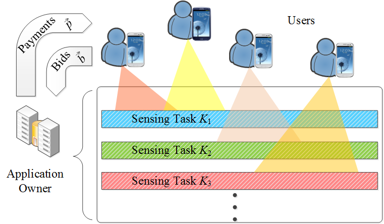
Figure 1: The mobile crowdsensing scheduling (MCS) problem.

2.2 Offline and Online Truthful Mechanisms

Each user $A_{i}$ has a utility indicating the difference between the payment made to him/her and his/her total sensing cost according to the sensing schedule, i.e., $p_{i}(\vec{b})-\hat{d}_{i}|y_{i}(\vec{b})|$. In practice, the users are selfish and are only interested in maximizing their own utilities. For this purpose, they may bid strategically, i.e., lying about their private information such as sensing costs and available time. To handle users’ strategic behaviors, we need to design truthful mechanisms for the MCS problem to align the users’ interests with the system goal of revenue maximization. A mechanism is called (dominant-strategy) truthful if any user maximizes his/her utility by revealing his/her real private information, no matter how other users may act [8]. A randomized mechanism is called truthful (or universally-truthful) if it is a randomization over a set of truthful mechanisms. Moreover, we also require our mechanisms to satisfy individual rationality (IR here after), which means that any truth-telling user $A_{i}$ always gets a non-negative utility [8], i.e., $p_{i}((\hat{d}_{i},\hat{s}_{i},\hat{e}_{i}),b_{-i})\geq\hat{d}_{i}|y_{i}((\hat{d}_{i},\hat{s}_{i},\hat{e}_{i}),b_{-i})|$, where $b_{-i}$ represents the bids of the users other than $A_{i}$.

In the following sections, we aim to design truthful mechanisms for the MCS problem under both the offline and online settings. In the offline setting, the owner collects all the users’ bids before scheduling them, which corresponds to a practical scenario that the users reserve sensing tasks in advance. In the online setting, the users’ bids are revealed one by one, and the owner must make an irrevocable decision on scheduling any user right at the moment when the user’s bid is revealed. This setting corresponds to another practical scenario where the users arrive randomly at some sensing area, and we assume that the users’ arrival order is drawn uniformly at random from the set of all permutations over the users.

3 Approximation Algorithms for MCS

In this section, we treat the MCS problem as a pure combinatorial optimization problem and design approximation algorithms for it, as shown in Algorithm 1. Although the strategic behaviors of the users are not considered in Algorithm 1, this algorithm serves as an important building block for the truthful mechanisms designed later.

1 $\mathcal{D}\leftarrow\mathcal{A}$;   $\mathcal{W}\leftarrow\emptyset$;    for $i\leftarrow 1$ to $n$ do  $y_{i}(\vec{b})\leftarrow\emptyset$ 

2 ;

3 repeat

4       Find $j$ such that $A_{j}=\max_{\prec}(\mathcal{D})$  

5       $Z_{j}\leftarrow T_{j}-\bigcup_{i:\kappa_{i}=\kappa_{j}}y_{i}(\vec{b})$

6       $q\leftarrow\min\left\{|Z_{j}|,\left\lfloor\frac{G}{2d_{j}}-\frac{R(\vec{y}(\vec{b}))}{\mu_{j}}\right\rfloor\right\}$  

7       if $q>0$ then

8             $\mathcal{W}\leftarrow\mathcal{W}\bigcup\{j\}$ 

9             $y_{j}(\vec{b})\leftarrow$ The first $q$ time units in $Z_{j}$  

10             $\mathcal{D}\leftarrow\mathcal{D}-\{A_{i}\in\mathcal{A}|T_{i}\subseteq\bigcup_{\ell:\kappa_{\ell}=\kappa_{i}}y_{\ell}(\vec{b})\}$ 

11            

12      

13until $q<|Z_{j}|$ or $\mathcal{D}=\emptyset$;

14 for $i\leftarrow 1$ to $n$ do  $p_{i}(\vec{b})\leftarrow d_{i}\cdot|y_{i}(\vec{b})|$  

15 ;

return $\vec{y}(\vec{b}),~{}\mathcal{W},~{}\vec{p}(\vec{b})$

Algorithm 1 $\mathsf{ApproxMCS}(n,G,\vec{b},\mathcal{A})$

A partial order $\prec$ on the set $\mathcal{A}$ is used in Algorithm 1, which is defined as follows. For any two users $A_{i}$ and $A_{j}$, if $\mu_{i}/d_{i}<\mu_{j}/d_{j}$ or $\mu_{i}/d_{i}=\mu_{j}/d_{j}$ but $j>i$, then we say $A_{j}$ suppress $A_{i}$ and denote it by $A_{i}\prec A_{j}$. For any $\mathcal{A}^{\prime}\subseteq\mathcal{A}$, we define $\max_{\prec}(\mathcal{A}^{\prime})$ to be the user in $\mathcal{A}^{\prime}$ such that there does not exist another user $\bar{A}\in\mathcal{A}^{\prime}$ satisfying $\max_{\prec}(\mathcal{A}^{\prime})\prec\bar{A}$.

Algorithm 1 iterates among the users and finds the schedule for them based on a greedy strategy. The algorithm, at the beginning of each iteration, selects a user $A_{j}$ based on the partial order $\prec$ (line 1), and then computes the time units that can potentially be scheduled for $A_{j}$ (line 1). The sensing time $y_{j}(\vec{b})$ scheduled for $A_{j}$ is taken as the early sub-period of the uncovered time of $A_{j}$, where any time point is called uncovered if no user has been scheduled for it (line 1). At the end of an iteration, all users whose available time periods have been covered are removed from the user set $\mathcal{D}$ upon which the algorithm iterates. The algorithm determines the length of $y_{j}(\vec{b})$ based on the rule in line 1, which can be deemed as a potential function [9] that facilitates our later quest for an approximation ratio. Also, the rule serves as a constraint to bound the total payments below $G$.

Let us denote an iteration (from line 1 to 1) in which line 1 is executed as an effective iteration (i.e., the concerned user is assigned a non-empty schedule). Suppose that Algorithm 1 has in total $h$ effective iterations. Let the user scheduled in the $i$th effective iteration be $A_{n_{i}}:1\leq i\leq h$ and let $\mathcal{W}=\{n_{1},n_{2},...,n_{h}\}$ be the index set of these scheduled users. Let $\vec{y}_{i}(\vec{b})$ be the current value of vector $\vec{y}(\vec{b})$ after the $i$th effective iteration is executed, we have the following results.

Theorem 2

The output of Algorithm 1 is a feasible solution to the MCS problem.

Theorem 3

Let $\vec{y}^{*}$ be an optimal schedule vector for the MCS problem and $\Lambda=\max_{i:d_{i}\leq G}(\mu_{i}\cdot|T_{i}|)$. If

$$\Lambda \leq \left[\frac{\mathbf{e}-1}{4\mathbf{e}}-\epsilon\right]R(\vec{y}^{*}),$$ (1)

for any $\epsilon\in(0,\frac{\mathbf{e}-1}{4\mathbf{e}})$, then $\vec{y}$ is a $\frac{4}{3}\epsilon$ approximation to MCS.

Note that an extra condition (1) needs to be satisfied in Theorem 3, hence the approximation ratio is conditional. We shall handle this issue using a randomized mechanism design method in the next section.

4 Offline Mechanisms for MCS

As users’ strategic behaviors are not considered in Algorithm 1, the payments to all users made there are directly determined by the declared sensing cost and the length of the time periods scheduled for them. Unfortunately, this method can be non-truthful: a user may lie about his/her private information to manipulate the length of his/her scheduled time, hence to gain a higher utility. Characterizations of truthful mechanisms exist in the literature (e.g., [10, 11]), but these characterizations are only for single parameter mechanisms, while in our problem any user $A_{i}$ has three parameters, namely $d_{i}$, $s_{i}$ and $e_{i}$. Therefore, we hereby design a novel truthful mechanism for the MCS problem under the offline setting, as shown by Algorithm 2. A sub-routine used by Algorithm 2 to compute payments to users is shown in Algorithm 3.

1 Generate a random number $o$ from the uniform distribution on the interval [0, 1] 

2 if $o\leq\frac{1}{2}$ then

3       $\left(\vec{y}(\vec{b}),\mathcal{W}\right)\leftarrow\mathsf{ApproxMCS}(n,G,\vec{b},\mathcal{A})$  

4       forall $n_{i}\in\mathcal{W}$ do

5             $p_{n_{i}}(\vec{b})\leftarrow\mathsf{CalPayment}(n,G,\vec{b},\mathcal{A},\mathcal{W},\vec{y},n_{i})$  

6            

7      forall $i\not\in\mathcal{W}$ do  $p_{i}(\vec{b})\leftarrow 0$ ;

8      

9else

10       forall $i\in\mathcal{A}$ do  $p_{i}(\vec{b})\leftarrow 0$  

11       ;

12       $j\leftarrow\arg\max_{i:d_{i}\leq G}\mu_{i}$;   $\mathcal{W}\leftarrow\{j\}$ 

13       $y_{j}(\vec{b})\leftarrow$ an arbitrary time unit in $T_{j}$;   $p_{j}(\vec{b})\leftarrow G$

14Pay $p_{i}(\vec{b})$ to $A_{i}\!:\forall i\in\mathcal{W}$ at the end of $T_{i}$ if $A_{i}$ successfully completes his/her sensing task during $y_{i}(\vec{b})$

return $\vec{y}(\vec{b}),~{}\vec{p}(\vec{b})$

Algorithm 2 Truthful Offline Mechanism for MCS

1 for $j\leftarrow 1$ to $n$ do  $t_{j}\leftarrow\emptyset$  

2 ;

3 for $j\leftarrow 1$ to $i-1$ do  $t_{n_{j}}\leftarrow y_{n_{j}}(\vec{b})$  

4 ;

5 $\mathcal{S}\leftarrow\{j|1\leq j\leq n,\frac{\mu_{j}}{d_{j}}\prec\frac{\mu_{n_{i}}}{d_{n_{i}}}\}$  

6 $p_{n_{i}}(\vec{b})\leftarrow d_{n_{i}}\cdot|y_{n_{i}}(\vec{b})|;~{}~{}~{}k\leftarrow n_{i};~{}~{}~{}\theta\leftarrow|\mathcal{S}|$

7 while $\theta\geq 0$ do

8       $\mathcal{Z}_{1}\leftarrow T_{n_{i}}-\bigcup_{\ell:\kappa_{n_{i}}=\kappa_{\ell}}t_{\ell}$; $\gamma_{1}\leftarrow\frac{\mu_{n_{i}}}{\mu_{k}}\cdot d_{k}$; $\gamma_{2}\leftarrow\frac{\mu_{n_{i}}G}{2R(\vec{t})}$  

9       if $\mathcal{S}\neq\emptyset$ then

10             Find $j$ such that $A_{j}=\max_{\prec}(\mathcal{S})$ 

11             $\gamma_{2}\leftarrow\min\left\{\frac{\mu_{n_{i}}}{\mu_{{j}}}\cdot d_{{j}},\gamma_{2}\right\}$ 

12            

13      if $|\mathcal{Z}_{1}|>0\bigwedge\gamma_{2}\geq\gamma_{1}$ then

14             $p_{n_{i}}(\vec{b})=p_{n_{i}}(\vec{b})\!+\!\int_{\gamma_{1}}^{\gamma_{2}}\min\left\{|\mathcal{Z}_{1}|,\left\lfloor\frac{G}{2v}-\frac{R(\vec{t})}{\mu_{n_{i}}}\right\rfloor\right\}\mathrm{d}v$

15      else $\mathbf{break}$;

16        

17       if $\mathcal{S}\neq\emptyset$ then

18             $\mathcal{Z}_{2}\leftarrow T_{j}-\bigcup_{\ell:\kappa_{j}=\kappa_{\ell}}t_{\ell}$ 

19             $q\leftarrow\min\left\{|\mathcal{Z}_{2}|,\left\lfloor\frac{G}{2d_{j}}-\frac{R(\vec{t})}{\mu_{j}}\right\rfloor\right\}$ 

20             if $q>0$ then

21                   $t_{j}\leftarrow$ The first $q$ time units in $Z_{2}$ 

22                  

23            if $q<|\mathcal{Z}_{2}|$ then $\mathbf{break}$;

24             

25             $k\leftarrow j;~{}~{}~{}\theta\leftarrow|\mathcal{S}|;~{}~{}~{}\mathcal{S}\leftarrow\mathcal{S}\backslash\{j\}$

26            

27      $\theta\leftarrow\theta-1$

return $p_{n_{i}}(\vec{b})$

Algorithm 3 $\mathsf{CalPayment}(n,G,\vec{b},\mathcal{A},\mathcal{W},\vec{y},n_{i})$

Algorithm 2 is apparently a randomized mechanism. With probability one half, the algorithm calls Algorithm 1 to get a feasible schedule for each user (line 2). However, instead of using the simple payment rule in Algorithm 1, Algorithm 2 replaces it with a more complicated method shown by Algorithm 3 to calculate the payments (line 2); otherwise Algorithm 2 runs lines 2-2 and selects a user whose sensing cost per unit time is no more than the budget and whose sensing value per unit time is maximized. Then the selected user is paid the amount $G$, while others are paid zero. The payments are made to the users using a post-paid scheme, i.e., a payment is made instantly at the end of a user’s claimed available time period only if he/she has successfully performed the sensing task during the whole time period scheduled for him/her (line 2). To understand the payment calculation in Algorithm 3, we introduce Lemma 1, Lemma 2 and Theorem 2, which are also useful for characterizing truthfulness under our multi-parameter environment.

Lemma 1

For any user $A_{i}$ and his/her two bids $b_{i}=(d_{i},s_{i},e_{i})$ and $b^{\prime}_{i}=(d_{i}^{\prime},s_{i},e_{i})$, if $d_{i}^{\prime}\geq d_{i}$, then $|y_{i}(b^{\prime}_{i},b_{-i})|\leq|y_{i}(b_{i},b_{-i})|$.

Lemma 2

For any user $A_{i}$ and his/her two bids $b_{i}=(d_{i},s_{i},e_{i})$ and $b^{\prime}_{i}=(d_{i},s^{\prime}_{i},e^{\prime}_{i})$, if $[s^{\prime}_{i},e^{\prime}_{i}]\subseteq[s_{i},e_{i}]$, then $|y_{i}(b^{\prime}_{i},b_{-i})|\leq|y_{i}(b_{i},b_{-i})|$.

Theorem 4

For any user $A_{i}$ with the bid $b_{i}=(d_{i},s_{i},e_{i})$ and any $b_{-i}$, $\int_{0}^{\infty}|y_{i}\left((v,s_{i},e_{i}),b_{-i}\right)|\mathrm{d}v<+\infty$ and the payment to $A_{i}$ computed by Algorithm 3 is

$$p_{i}(b_{i},b_{-i})=d_{i}|y_{i}(b_{i},b_{-i})|+\!\int_{d_{i}}^{\infty}\!\!|y_{i}\left((v,s_{i},e_{i}),b_{-i}\right)|\mathrm{d}v.$$ (2)

Proof:

For $i\not\in\{n_{1},n_{2},...,n_{h}\}$, we have $p_{i}(b_{i},b_{-i})=0$ and $|y_{i}(b_{i},b_{-i})|=0$. According to Lemma 1, for any $v>d_{i}$, we have $|y_{i}((v,s_{i},e_{i}),b_{-i})|\leq|y_{i}(b_{i},b_{-i})|$, hence $|y_{i}((v,s_{i},e_{i}),b_{-i})|=0$. So (2) holds in this case.

Now we analyze Algorithm 3 in details for the case of $i\in\{n_{1},n_{2},...,n_{h}\}$, and we write $i$ as $n_{i}$ in this case. In Algorithm 3, we first initialize the vector $\vec{t}$ to record the user schedules that are decided before $A_{n_{i}}$, as shown in lines 3-3. Then we use $\mathcal{S}$ to denote the indices of the users that are suppressed by $A_{n_{i}}$ according to the partial order $\prec$ (line 3). Note that if $A_{n_{i}}$ bids $d^{\prime}_{n_{i}}>d_{n_{i}}$, the uncovered available time period of $A_{n_{i}}$ (i.e., $\mathcal{Z}_{1}$) may change, because we have $\mu_{n_{i}}/d^{\prime}_{n_{i}}<\mu_{n_{i}}/d_{n_{i}}$ and some users originally suppressed by $A_{n_{i}}$ may hence get scheduled before $A_{n_{i}}$. Consequently, we calculate the schedule for other users (recorded in $\vec{t}$) when $d_{n_{i}}$ increases, and divide the interval $[d_{n_{i}},+\infty)$ into some sub-intervals, such that the uncovered available time period of $A_{n_{i}}$ remains the same when $A_{n_{i}}$ changes $d_{n_{i}}$ within each of these sub-intervals, as shown in lines 3-3. More specifically, the algorithm, at the beginning of each iteration, picks a user’s index $j$ from $\mathcal{S}$ such that $A_{j}$ is maximal with respect to the partial order $\prec$, then it identifies a sub-interval $\left(\left.\frac{\mu_{n_{i}}}{\mu_{{k}}}\cdot d_{{k}},\frac{\mu_{n_{i}}}{\mu_{{j}}}\cdot d_{{j}}\right]\right.$ for $d_{n_{i}}$ (indicated by $\gamma_{1}$ and $\gamma_{2}$), where $k$ is the index of the last picked user from $\mathcal{S}$ (line 3, but initially set as $n_{i}$). As $A_{n_{i}}$ remains scheduled before $A_{j}$ when $d_{n_{i}}$ varies within this sub-interval, we calculate the partial payment in line 3 based on the current schedule. When $d_{n_{i}}$ gets bigger than $\frac{\mu_{n_{i}}}{\mu_{{j}}}\cdot d_{{j}}$, then $A_{j}$ will be scheduled before $A_{n_{i}}$, and we calculate $A_{j}$’s schedule in this case by lines 3-3. With this adjusted schedule, the algorithm goes into the next iteration to further accumulate the partial payment in a different sub-interval. At the end, the algorithm goes through all the possible sub-intervals in $[d_{n_{i}},\infty)$, so the payment is exactly calculated as the right-hand side of (2). Hence the theorem follows. ∎

In Lemma 3 and Theorem 5, we prove that the payment calculated by Algorithm 3 is no more than the budget $G$ and Algorithm 2 provides a feasible solution satisfying IR to the MCS problem.

Lemma 3

For any user $A_{j}$ and his/her bid $(d_{j},s_{j},e_{j})$, if $j\in\{n_{1},n_{2},...,n_{h}\}$, then we have $d_{j}\leq\mu_{j}\cdot G/R(\vec{y})$.

Theorem 5

The mechanism shown in Algorithm 2 provides a feasible solution that satisfies IR to the MCS problem.

More importantly, using the results stated in Lemma 1, Lemma 2 and Theorem 2, we can now prove the truthfulness of the mechanism by Theorem 6. The rationale lies in the difference between any user $A_{i}$’s payment and his/her true sensing cost: regardless of how other users may bid, this difference is always maximized if $A_{i}$ bids truthfully and hence truth-telling is a dominant strategy for $A_{i}$.

Theorem 6

The scheduling mechanism shown in Algorithm 2 is truthful.

Proof:

We first prove that lines 2-2 is truthful. Suppose that there exists a user $A_{i}$ whose truthful bid is $\hat{b}_{i}=(\hat{d}_{i},\hat{s}_{i},\hat{e}_{i})$, but he/she can get a higher utility by bidding $b_{i}=(d_{i},s_{i},e_{i})\neq\hat{b}_{i}$ for some $b_{-i}$. If $y_{i}(b_{i},b_{-i})\not\subseteq[\hat{s}_{i},\hat{e}_{i}]$, $A_{i}$ gets zero payment because the mechanism requires $A_{i}$ to complete sensing during $y_{i}(b_{i},b_{-i})$ to get paid. If $e_{i}\not\in[\hat{s}_{i},\hat{e}_{i}]$, $A_{i}$ again gets zero payment because the mechanism employs a post-paid scheme and $A_{i}$ cannot get paid when he/she is unavailable. Therefore, we must have $y_{i}(b_{i},b_{-i})\subseteq[\hat{s}_{i},\hat{e}_{i}]$ and $e_{i}\in[\hat{s}_{i},\hat{e}_{i}]$. Now if $s_{i}\geq\hat{s}_{i}$, we have $[s_{i},e_{i}]\subseteq[\hat{s}_{i},\hat{e}_{i}]$; so using Lemma 2 we get

$$|y_{i}\left((d_{i},s_{i},e_{i}),b_{-i}\right)| \leq |y_{i}\left((d_{i},\hat{s}_{i},\hat{e}_{i}),b_{-i}\right)|.$$ (3)

Otherwise if $s_{i}<\hat{s}_{i}$, we know that the period $[s_{i},\hat{s}_{i}]$ must have been covered before deciding the schedule of $A_{i}$ based on his/her bidding $b_{i}$, because otherwise the algorithm will allocate time in $[s_{i},\hat{s}_{i}]$ to $A_{i}$ according to line 1 of Algorithm 1, which contradicts $y_{i}(b_{i},b_{-i})\subseteq[\hat{s}_{i},\hat{e}_{i}]$. Hence we know $y_{i}\left((d_{i},s_{i},e_{i}),b_{-i}\right)=y_{i}\left((d_{i},\hat{s}_{i},e_{i}),b_{-i}\right)$. As $[\hat{s}_{i},e_{i}]\subseteq[\hat{s}_{i},\hat{e}_{i}]$, (3) also holds by using Lemma 2.

For $A_{i}$’s any bid $(d^{\prime}_{i},s^{\prime}_{i},e^{\prime}_{i})$, let $f_{i}((d^{\prime}_{i},s^{\prime}_{i},e^{\prime}_{i}),b_{-i})$ denote the uncovered time in $[s^{\prime}_{i},e^{\prime}_{i}]$ when the algorithm allocates time to $A_{i}$ based on a bid vector $((d^{\prime}_{i},s^{\prime}_{i},e^{\prime}_{i}),b_{-i})$. The above reasoning actually reveals that $f_{i}((d_{i},s_{i},e_{i}),b_{-i})\subseteq f_{i}((d_{i},\hat{s}_{i},\hat{e}_{i}),b_{-i})$. According to the mechanism, for any $v\geq d_{i}$ we have $f_{i}((v,s_{i},e_{i}),b_{-i})\subseteq f_{i}((d_{i},s_{i},e_{i}),b_{-i})$, $f_{i}((v,\hat{s}_{i},\hat{e}_{i}),b_{-i})\subseteq f_{i}((d_{i},\hat{s}_{i},\hat{e}_{i}),b_{-i})$ and

$$[f_{i}((d_{i},\hat{s}_{i},\hat{e}_{i}),b_{-i})\backslash f_{i}((v,\hat{s}_{i},\hat{e}_{i}),b_{-i})]\cap f_{i}((d_{i},s_{i},{e}_{i}),b_{-i})$$

$$\subseteq f_{i}((d_{i},{s}_{i},{e}_{i}),b_{-i})\backslash f_{i}((v,{s}_{i},{e}_{i}),b_{-i}),$$

which yield $f_{i}((v,s_{i},e_{i}),b_{-i})\subseteq f_{i}((v,\hat{s}_{i},\hat{e}_{i}),b_{-i})$ and

$$|y_{i}\left((v,s_{i},e_{i}),b_{-i}\right)| \leq |y_{i}\left(((v,\hat{s}_{i},\hat{e}_{i}),b_{-i}\right)|.$$ (4)

Since the user gets more utility by bidding $b_{i}$ then by bidding $\hat{b}_{i}$, we know that:

$$p_{i}((d_{i},s_{i},e_{i}),b_{-i})-\hat{d}_{i}\cdot|y_{i}((d_{i},s_{i},e_{i}),b_{-i})|$$

$$> p_{i}((\hat{d}_{i},\hat{s}_{i},\hat{e}_{i}),b_{-i})-\hat{d}_{i}\cdot|y_{i}((\hat{d}_{i},\hat{s}_{i},\hat{e}_{i}),b_{-i})|.$$

Combing this with Theorem 2 gives us

$$(d_{i}-\hat{d}_{i})\cdot|y_{i}((d_{i},s_{i},e_{i}),b_{-i})|$$

$$> \int_{\hat{d}_{i}}^{\infty}|y_{i}((v,\hat{s}_{i},\hat{e}_{i}),b_{-i})|\mathrm{d}v-\int_{d_{i}}^{\infty}|y_{i}((v,s_{i},e_{i}),b_{-i})|\mathrm{d}v.$$

Case 1: $d_{i}\geq\hat{d}_{i}$, using (4) and Lemma 1 we get

$$(d_{i}-\hat{d}_{i})\cdot|y_{i}((d_{i},s_{i},e_{i}),b_{-i})|$$

$$> \int_{\hat{d}_{i}}^{d_{i}}|y_{i}((v,\hat{s}_{i},\hat{e}_{i}),b_{-i})|\mathrm{d}v$$

$$\geq (d_{i}-\hat{d}_{i})\cdot|y_{i}((d_{i},\hat{s}_{i},\hat{e}_{i}),b_{-i})|.$$

If $d_{i}=\hat{d}_{i}$, then we get $0>0$, a contradiction. If $d_{i}>\hat{d}_{i}$, then we get $|y_{i}((d_{i},s_{i},e_{i}),b_{-i})|>|y_{i}((d_{i},\hat{s}_{i},\hat{e}_{i}),b_{-i})|$, which contradicts (3).

Case 2: $d_{i}<\hat{d}_{i}$, using (4) and Lemma 1 we get:

$$(d_{i}-\hat{d}_{i})\cdot|y_{i}((d_{i},s_{i},e_{i}),b_{-i})|$$

$$> -\int_{d_{i}}^{\hat{d}_{i}}|y_{i}((v,s_{i},e_{i}),b_{-i})|\mathrm{d}v$$

$$\geq (d_{i}-\hat{d}_{i})\cdot|y_{i}((d_{i},s_{i},e_{i}),b_{-i})|,$$

hence $|y_{i}((d_{i},s_{i},e_{i}),b_{-i})|<|y_{i}((d_{i},s_{i},e_{i}),b_{-i})|$, also a contradiction.

The above reasoning has shown that lines 2-2 is truthful. Now we prove that lines 2-2 is truthful. If a user $A_{i}$ gets a non-empty schedule by bidding truthfully, then $A_{i}$ clearly cannot benefit from lying. Now suppose that $A_{i}$ gets an empty schedule (hence the utility 0) by bidding truthfully. If $\hat{d}_{i}\leq G$, then $A_{i}$ cannot increase his/her utility by lying, because he/she will anyway get an empty schedule regardless of his/her bid. If $\hat{d}_{i}>G$, then the only way that may allow $A_{i}$ to get a non-empty schedule is to bid some $(d_{i},s_{i},e_{i})$ with $d_{i}\leq G$. However, in that case $A_{i}$’s utility is $G-\hat{d}_{i}<0$. Therefore, $A_{i}$ is better off bidding truthfully. From the above reasoning, we know that Algorithm 2 is a randomization of two truthful mechanisms, and is hence truthful. ∎

Finally, based on the approximation ratio of Algorithm 1, we can prove that Algorithm 2 has an $\mathcal{O}(1)$ approximation ratio, as shown by Theorem 7. We also analyze the time complexity of Algorithm 2 by Theorem 8.

Theorem 7

The mechanism shown in Algorithm 2 has an approximation ratio of $\mathcal{O}(1)$.

Theorem 8

The worst-case time complexity of Algorithm 2 is $\mathcal{O}(n^{2})$.

Obviously, the major time complexity results from calling Algorithm 3 for at most $n$ times.

5 Online Mechanisms for MCS

In this section, we study incentive mechanisms for the MCS problem under the online setting, where the users come in random orders and the schedule/payment for each user has to be decided upon his/her arrival. We assume in this case that any user $A_{i}$ would only lie about his/her sensing cost $\hat{d}_{i}$, and we will design truthful mechanisms such that reporting his/her real cost is a dominant strategy of $A_{i}$. The problem of handling users’ strategic bidding on their available time periods under the online setting is left for future work.

We first propose a simple online mechanism in Algorithm 4 for the MCS problem, whose idea originates from the secretary algorithm [12].

1 $\alpha\leftarrow 0$;   $j\leftarrow 0$

2 upon $A_{i}$’s arrival

3       $j\leftarrow j+1$

4       if $j\leq\lfloor\frac{n}{\mathbf{e}}\rfloor$ then

5             $y_{i}\leftarrow\emptyset$;   $p_{i}\leftarrow 0$

6             if $d_{i}\leq G$ then  $\alpha\leftarrow\max\{\alpha,\mu_{i}\}$ ;

7            

8      else

9             if $\mu_{i}\geq\alpha\bigwedge d_{i}\leq G\bigwedge G>0$ then

10                   $y_{i}\leftarrow$ an arbitrary time unit in $T_{i}$

11                   $p_{i}\leftarrow G$;   $G\leftarrow 0$

12                  

13            else

14                   $y_{i}\leftarrow\emptyset$;   $p_{i}\leftarrow 0$

15            

16      

17

return $(\vec{y},\vec{p})$

Algorithm 4 A Deterministic Online Mechanism

In lines 4-4 of Algorithm 4, we assign empty schedules to the first arrived $\lfloor\frac{n}{\mathbf{e}}\rfloor$ users, and find one of them whose sensing cost per unit time is no more than the budget and whose sensing value per unit time is the maximum denoted by $\alpha$. The value of $\alpha$ is then used as a threshold for the later users, among which we will select the first one whose sensing value per unit time is no less than $\alpha$ and pay him/her $G$; other users all get empty schedules and zero payments (lines 4-4). The schedules and payments assigned to the users are returned by vector $\vec{y}$ and vector $\vec{p}$, respectively.

Clearly, Algorithm 4 provides a feasible solution to the MCS problem and satisfies IR. The truthfulness and competitive ratio of Algorithm 4 are given in Theorem 9 and Theorem 10, respectively:

Theorem 9

The online scheduling mechanism in Algorithm 4 is truthful.

Proof:

As the users cannot control their arrival sequence, they also cannot control the value of $\alpha$. The first arrived $\lfloor\frac{n}{\mathbf{e}}\rfloor$ users are always assigned the empty schedule, so they always get the utility 0 no matter how they bid. Now consider any $A_{i}$ whose arrival order is greater than $\lfloor\frac{n}{\mathbf{e}}\rfloor$. If $A_{i}$ gets a non-empty schedule by bidding $\hat{d}_{i}$, then it is clear that he/she cannot benefit from lying, because his/her utility $G-\hat{d}_{i}\geq 0$ is the largest one he/she can possibly get. Otherwise if $A_{i}$ gets an empty schedule by bidding $\hat{d}_{i}$, then there are two cases we need to consider: (i) $G=0$ when $A_{i}$ arrives: In this case, $A_{i}$ will always get utility 0 no matter how he/she bids. (ii) $G>0$ when $A_{i}$ arrives: In this case we must have $\mu_{i}<\alpha$ or $\hat{d}_{i}>G$. If $\mu_{i}<\alpha$, then $A_{i}$ always gets utility 0 regardless of his/her bid. If $\mu_{i}\geq\alpha$ and $\hat{d}_{i}>G$, bidding any $d_{i}>G$ will always cause $A_{i}$ to get an empty schedule (hence the utility 0), while bidding $d_{i}\leq G$ would enable $A_{i}$ to get a non-empty schedule, but his/her utility $G-\hat{d}_{i}$ would be negative; hence he/she is better off bidding truthfully. ∎

Theorem 10

If $\Lambda\geq\frac{R(\vec{y}^{*})}{150}$ (where $\Lambda$ was defined in Theorem 3), then Algorithm 4 has a $\mathcal{O}(1)$ competitive ratio with a constant probability.

Note that the competitive ratio stated in Theorem 10 is conditional. To rectify this problem, we propose a randomized mechanism shown in Algorithm 5, which runs Algorithm 4 with probability one half and runs lines 5-5 otherwise. Roughly speaking, the idea of lines 5-5 is the following: we assign the empty schedule to the first arrived $\xi$ users and use them as a random sample to guess the optimal solution $R(\vec{y}^{*})$ (lines 5-5); then we use this guess to schedule the users coming afterwards (lines 5-5).

1 Generate a random number $o$ from the uniform distribution on the interval [0, 1];

2 if $o\leq\frac{1}{2}$ then

3       Let $\xi$ be a random number generated from the binomial distribution $B(n,1/2)$

4       $M\leftarrow G$;   $j\leftarrow 0$;   $\mathcal{A}_{\xi}\leftarrow\emptyset$

5       upon $A_{i}$’s arrival

6             $j\leftarrow j+1$

7             if $j\leq\xi$ then

8                   $y_{i}\leftarrow\emptyset$;   $p_{i}\leftarrow 0$;   $\mathcal{A}_{\xi}\leftarrow\mathcal{A}_{\xi}\bigcup\{A_{i}\}$

9                   if $j=\xi$ then

10                         $\vec{r}(\vec{b}_{\xi})\leftarrow\mathsf{ApproxMCS}(\xi,G,\vec{b}_{\xi},\mathcal{A}_{\xi})$

11                        

12                  

13            else

14                   $\eta\leftarrow 5G\cdot\mu_{i}/R(\vec{r})$;   $F_{i}\leftarrow T_{i}-\bigcup_{\ell:\kappa_{i}=\kappa_{\ell}}y_{\ell}$

15                   if $d_{i}\leq\eta\bigwedge\eta\cdot|F_{i}|\leq M\bigwedge|F_{i}|\geq 1$ then

16                         $y_{i}\leftarrow F_{i}$;   $p_{i}\leftarrow\eta\cdot|F_{i}|$;   $M\leftarrow M-p_{i}$

17                        

18                  else

19                         $y_{i}\leftarrow\emptyset$;   $p_{i}\leftarrow 0$

20                  

21            

22      

23else  Run Algorithm 4 to get $(\vec{y},\vec{p})$

24 ;

return $(\vec{y},\vec{p})$

Algorithm 5 A Randomized Online Mechanism

It can be seen from lines 5-5 that Algorithm 5 satisfies IR and provides a feasible solution to the MCS problem. The truthfulness of Algorithm 5 is proven in Theorem 11:

Theorem 11

The online scheduling mechanism shown in Algorithm 5 is truthful.

Proof:

We have proved in Theorem 9 that Algorithm 4 is truthful, so we only need to prove that lines 5-5 are truthful given that users strategically report their sensing costs. Note that the users cannot control their arrival order as well as the value of $R(\vec{r})$, hence the first arrived $\xi$ users always get utility $0$ no matter how they bid. Now consider any user $A_{i}$ who arrives afterwards. If $A_{i}$ gets a non-empty schedule (i.e., $|y_{i}|\neq 0$) by bidding $\hat{d}_{i}$, then we know that $\hat{d}_{i}\leq\eta$ and $A_{i}$ gets the utility $(\eta-\hat{d}_{i})\cdot|F_{i}|\geq 0$, which remains the same if $A_{i}$ bids any $d_{i}\leq\eta$. If $A_{i}$ bids $d_{i}>\eta$, then his/her utility will be $0$, so he/she is better off bidding his/her true value. Otherwise if $|y_{i}|=0$ when $A_{i}$ bids $\hat{d}_{i}$, then at least one of the following conditions holds: (i) $\eta\cdot|F_{i}|>M$; (ii) $|F_{i}|=0$; (iii) $\hat{d}_{i}>\eta$. If (i) or (ii) holds, $A_{i}$’s utility remains $0$ no matter how he/she bids. If (iii) holds, then bidding $d_{i}\leq\eta$ may get $A_{i}$ assigned a non-empty schedule, but in that case the utility of $A_{i}$ would be $(\eta-\hat{d}_{i})\cdot|F_{i}|<0$, hence he/she is still better off bidding the true value $\hat{d}_{i}$. ∎

Finally, the competitive ratio and time complexity of Algorithm 5 are given in Lemma 4-6 and Theorem 12:

Lemma 4

Let $(\sigma_{1},\sigma_{2},...,\sigma_{n})$ be the actual arrival sequence of the users’ indices, which is a permutation of $\{1,2,...,n\}$. Let $\Delta_{1}=\sum_{i=1}^{\xi}\mu_{\sigma_{i}}\cdot|y^{*}_{\sigma_{i}}|$ and $\Delta_{2}=\sum_{i=\xi+1}^{n}\mu_{\sigma_{i}}\cdot|y^{*}_{\sigma_{i}}|$. If $\Lambda\leq\frac{R(\vec{y}^{*})}{150}$, then $\Delta_{1}\geq{R(\vec{y}^{*})}/{3}$ and $\Delta_{2}\geq{R(\vec{y}^{*})}/{4}$ hold at the same time with constant probability.

Lemma 5

If $\Lambda\leq\frac{R(\vec{y}^{*})}{150}$, then $\frac{\Delta_{1}}{5}\leq R(\vec{r})\leq R(\vec{y}^{*})$.

Lemma 6

If $\Lambda\leq\frac{R(\vec{y}^{*})}{150}$, then the solution output by lines 5-5 of Algorithm 5 has an $\mathcal{O}(1)$ competitive ratio with constant probability.

Theorem 12

The competitive ratio and worst-case time complexity of Algorithm 5 are $\mathcal{O}(1)$ and $\mathcal{O}(n^{2})$, respectively.

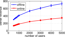
(a) Revenue changing with user number.

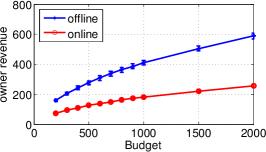
(b) Revenue changing with budget.

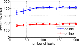
(c) Revenue changing with task number

Figure 2: The owner’s revenue as functions of (a) the number of users, (b) the total budget, and (c) the number of tasks.

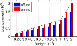
(a) Payment changing with budget.

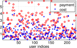
(b) IR validation for offline.

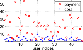
(c) IR validation for online.

Figure 3: Feasibility check in terms of total payment and IR.

6 Simulations

We conduct extensive simulations to evaluate the performance of our truthful scheduling mechanisms. The objective of our simulations is to corroborate the correctness and effectiveness of our mechanisms in terms of various metrics (including owner revenue, total payment, truthfulness and IR) under different parameter settings (such as the number of users or tasks, as well as the budget). Since we are the first, to the best of our knowledge, to study the MCS problem (see the discussions in Sec. 1 and the definition in Sec. 2), we can only make comparisons between our own algorithms in the simulations. For brevity, we hereby denote our two main algorithms Algorithm 2 and Algorithm 5 by “offline” and “online”, respectively.

6.1 Default Settings

We randomly generate the sensing values of tasks, the number of users and the users’ private values. More specifically, the sensing cost per unit time (i.e., $\hat{d}_{i}$) of any user $A_{i}$ is generated randomly from the uniform distribution $U[0.1,1.1]$, and the sensing value per unit time $u_{i}$ of any task $K_{i}$ is also generated from the same distribution (i.e., both are bounded away from 0). The earliest available time point $\hat{s}_{i}$ of any user $A_{i}$ is generated randomly from $U[0,100]$, whereas the length of $A_{i}$’s available time period is generated randomly from $U[0,10]$. Both the number of users $n$ and the budget $G$ are set to 1000; the number of tasks $m$ is set 100; and each user selects only one task, with equal probability out of all tasks. All our simulations follow these default settings unless otherwise stated.

6.2 Owner Revenue

We study the owner revenue achieved by our mechanisms under different user number, budget and task number in Fig. 2. For each data point, we perform 100 simulations with random inputs and we plot the average value and standard deviation. In general, offline always works better than online. This is natural because online faces a harsher condition that a schedule has to be determined for a user upon his/her arrival. In particular, with the information on all users, offline can leverage a sorting based on $\prec$ to optimize the performance, whereas online do not have this privilege.

In Fig. 2(a), we study the impact of the number of users on the owner revenue, by scaling the number of users from 500 to 5000 with an increment of 100 (below 1000) and of 1000 (beyond 1000). The owner revenues of both offline and online increase with the number of users. This can be explained by the reason that, as the diversities of both the users’ sensing costs and available time periods increase with the number of users, the degree of freedom in finding schedules is enlarged, which in turn results in larger revenues. The same trend is also shown in Fig. 2(b), where we fix the number of users to 1000 but scale the budget $G$ from 200 to 2000 with an increment of 100 (before 1000) and of 500 (after 1000). This is rather straightforward to understood because a higher budget allows the algorithms to schedule users whose sensing costs are higher and hence cannot be afforded under a lower budget.

In Fig. 2(c), we fix the user number to 1000 and increase the number of tasks from 20 to 200 with an increment of 20. It can be seen that the owner revenues obtained by both our mechanisms slightly increase when the number of tasks increases. This can be explained by the reason that, when the number of tasks increases, the number of users that can perform each task tend to decrease, which results in less overlapping available time periods and higher revenue. Obviously, this effect is less direct than that from either increasing user number or budget, so the resulting improvement to the revenue is also marginal.

6.3 Solution Feasibility and Individual Rationality

We verify the feasibility and IR of the solutions output by our algorithms in this section. We first show that the total payment is always no more than the budget, then we use two examples to demonstrate that IR is also guaranteed, i.e., each user gets a payment higher than his/her cost. In Fig. 3(a), we scale the budget in the same way as Fig. 2(b), and we show the maximum total payment for each case. Apparently, the budget has never been surpassed. Again, offline is shown to be superior to online: it results in lower total payments.

In Fig. 3(b) and 3(c), we demonstrate IR using the outputs from offline and online, respectively. We plot the sensing costs and payments only for users with non-zero payments. IR of our mechanisms can be immediately seen: a payment is always greater than the corresponding cost. We can also see that more users are assigned non-empty schedules by offline, which, to some extent, explains the observation made for Fig. 2 that offline always achieves a higher revenue than online.

6.4 Truthfulness

We verify the truthfulness of both offline and online by arbitrarily picking up a few users and checking their utilities under different bidding values.

We first study the truthfulness of offline by Fig. 4. We arbitrarily pick a user $A_{i}$ whose true values are $\hat{d}_{i}=0.5$, $\hat{s}_{i}=12$ and $\hat{e}_{i}=22$, then we change $A_{i}$’s bid (with other users’ bids fixed) to see how $A_{i}$’s utility changes. Since we cannot draw a 4-dimensional chart here, we show the results by two figures. In Fig. 4(a), the bid of $A_{i}$’s available time period is fixed to $[12,22]$, and we scale $A_{i}$’s bid on his sensing cost from 0.1 to 3.3 with an increment of 0.1. Indeed, bidding the true sensing cost (shown by the red pentagram) allows $A_{i}$ to maximize his/her utility. In Fig. 4(b), we fix $A_{i}$’s bid on his sensing cost to 0.5, but varies $A_{i}$’s bid on his earliest and latest available time points. Again, $A_{i}$’s utility is maximized when he/she bids his/her true value $[12,22]$. These demonstrate that $A_{i}$ has no incentive to deviate from bidding his/her true values.

Similarly, we study the truthfulness of online by Fig. 5. In Fig. 5(a), we pick an arbitrary user whose true sensing cost is 0.3 and who is assigned an empty schedule by online. Then we scale this user’s bid on his sensing cost from 0.01 to 0.4 with an increment of 0.01. The user indeed achieves his/her maximum utility 0 by bidding his true sensing cost 0.3. In Fig. 5(b), we pick another user (in another simulation) whose true sensing cost is 0.4 and who is assigned a non-empty schedule by online. Then we scale this user’s bid from 0.01 to 10 with an increment of 0.01. Again, the result shows that the user’s utility is maximized when he/she bids his/her true sensing cost.

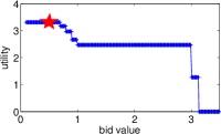
(a) Truthfulness on the sensing cost.

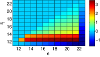
(b) Truthfulness on the available time.

Figure 4: Truthfulness validation for offline.

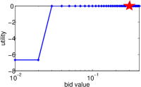
(a) Truthfulness for a user $A_{i}$ who gets an empty schedule.

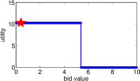
(b) Truthfulness for a user $A_{i}$ who gets a non-empty schedule.

Figure 5: Truthfulness validation for online.

7 Related Work

Mobile crowdsensing involves using (human carried) smartphones to gather data in a much larger scale than what can be done in conventional ways, either through autonomous phone sensing or by further demanding active human participation[1, 2]. While the developments on mobile crowdsensing applications are plentiful, only a few proposals have started on studying how to incentivize participation to such applications until very recently [3, 4, 5, 6, 7].

Duan et al. [5] have proposed incentive mechanisms to motivate collaboration in mobile crowdsensing based on Stackelberg games and contract theory. However, the mechanisms provided in [5] require either the complete information or the prior distributions of users’ private types, hence are not prior-free mechanisms as those in our work. Yang et al. [6] suggest both a platform-centric model and a user-centric model for mobile sensing. They also use a Stackelberg game to design incentive mechanisms for the platform-centric model, and use auction theory to design truthful mechanisms for the user-centric model; nevertheless the truthful auction mechanisms provided in [6] are only for single-parameter users and only run in an offline manner. Moreover, no theoretical performance ratios are provided for them in [6]. Some other issues such as pricing, coverage, and privacy of mobile crowdsensing have also been studied by the work in [3, 4, 7], but these proposals are either not based on a game theoretical perspective or have not considered important game-theoretic issues such as truthfulness and IR. Most importantly, none of the work in [3, 4, 5, 6, 7] has considered the special time scheduling problem arising from the mobile crowdsensing paradigm, hence their problem definitions are totally different from ours.

There also exist proposals on designing approximation algorithms or truthful mechanisms for job-scheduling on parallel machines, such as [13, 14, 15, 16]. However, these proposals focus on the problem of minimizing the scheduling makespan, which is a totally different goal from ours. Besides, all the mechanisms in this line could entail an arbitrarily large payment to ensure truthfulness. Finally, the frugal or budget-feasible mechanism design problems have been studied in [17, 18, 19, 20], but these proposals only aim at designing single-parameter mechanisms for allocating indivisible goods, which is very different from the scheduling problems studied in this paper.

8 Conclusion

We have studied incentive mechanisms for a novel scheduling problem (the MCS problem) arising from the mobile crowdsensing paradigm, where an application owner pays the sensor carriers and schedules their sensing time based on their bids to maximize the total sensing value. We have proved the NP-hardness of the MCS problem, and proposed polynomial-time approximation mechanisms for it that run both offline and online. We also have proved that our mechanisms have $\mathcal{O}(1)$ performance ratios and satisfies game-theoretic properties including individual rationality and truthfulness. The effectiveness of our approach has been corroborated by the simulation results. To the best of our knowledge, we are the first to study the mechanism design problems for the mobile crowdsensing scheduling problem.

Proof:

We prove the NP-hardness of the MCS problem by a reduction from the Partition problem [21]. Given a set of $n$ integers $S=\{a_{1},a_{2},...,a_{n}\}$, the Partition problem is to decide whether the set $S$ can be partitioned into two subsets such that the sum of the numbers in one subset equals the sum of the numbers in another. Suppose that there are $n$ tasks and $n$ users in the MCS problem, and each user $A_{i}$ can perform only task $K_{i}$. Let the length of the available time period of any user be $1$, and let $a_{i}=d_{i}=\mu_{i}$ for any $i$. Let the budget $G=\frac{1}{2}\sum_{i=1}^{n}a_{i}$. The MCS decision problem asks if the owner can obtain a revenue $R\geq G$. Obviously, this problem is equivalent to the Partition problem on the set $S$. Since the Partition problem is NP-complete, the MCS problem is NP-hard. ∎

Proof:

As the users’ strategic behaviours are not considered here, it can be easily seen by line 1 in Algorithm 1 that any user can always get a payment no less than his sensing cost. Hence we only need to prove that the total amount paid to the users is no more than the budget $G$. For any $1\leq i\leq h$ we have

$$R(\vec{y}_{i}) = R(\vec{y}_{{i-1}})+|y_{n_{i}}|\mu_{n_{i}}$$

$$\leq R(\vec{y}_{{i-1}})+\mu_{n_{i}}\left(\frac{G}{2d_{n_{i}}}-\frac{R(\vec{y}_{{i-1}})}{\mu_{n_{i}}}\right)$$

$$= {\mu_{n_{i}}G}/({2d_{n_{i}}}),$$

hence we get

$${\mu_{n_{i}}}/{d_{n_{i}}} \geq {2R(\vec{y}_{i})}/{G},$$ (5)

and

$${\mu_{n_{1}}}/{d_{n_{1}}}\geq{\mu_{n_{2}}}/{d_{n_{2}}}\geq\cdots\geq{\mu_{n_{h}}}/{d_{n_{h}}}\geq{2R(\vec{y})}/{G}.$$

So the total amount paid to the users is

$$\sum_{1\leq i\leq h}d_{n_{i}}\cdot|y_{n_{i}}|~{}~{}\leq~{}~{}\sum_{1\leq i\leq h}\mu_{n_{i}}\cdot|y_{n_{i}}|\cdot\frac{G}{2R(\vec{y})}~{}~{}=~{}~{}\frac{G}{2}.$$ (6)

Therefore, Algorithm 1 yields a feasible solution. ∎

Proof:

Suppose that Algorithm 1 has $l$ effective iterations if we replace line 1 by

$$q\leftarrow\min\left\{|Z_{j}|,\frac{G-\sum_{i=1}^{n}d_{i}*|w_{i}(\vec{b})|}{d_{j}}\right\},$$ (7)

and let $\vec{x}_{i}$ be the current vector $\vec{w}(\vec{b})$ after the $i$th effective iteration ($1\leq i\leq l$) is executed in this case. Clearly, $h\leq l$, and the user scheduled in the $i$th effective iteration under this case can also be denoted by $A_{n_{i}}:1\leq i\leq l$. Let $R^{\prime}(\vec{x}_{i})=\sum_{j=1}^{i}\mu_{n_{j}}|x_{n_{j}}|$.

Let $\mathcal{X}_{0}=\emptyset$ and $\mathcal{X}_{i}=\{A_{n_{1}},A_{n_{2}},...,A_{n_{i}}\}$ for any $1\leq i\leq l$. From Algorithm 1 we know that, for any $1\leq j<l$ and any $1\leq i\leq j$, $T_{n_{i}}$ must be covered by $\vec{x}_{j}$, i.e., $T_{n_{i}}\subseteq\bigcup_{1\leq\ell\leq j\wedge\kappa_{n_{\ell}}=\kappa_{n_{i}}}f_{n_{\ell}}$ where $\vec{f}=\vec{x}_{j}$. Therefore, we have

$$R(\vec{w}^{*})-R^{\prime}(\vec{x}_{j})\leq\sum\nolimits_{i:A_{i}\in\mathcal{A}\backslash\mathcal{X}_{j}}|w^{*}_{i}|\mu_{i}$$ (8)

$$= \sum\nolimits_{i:A_{i}\in\mathcal{A}\backslash\mathcal{X}_{j}}|w^{*}_{i}|d_{i}\cdot\frac{\mu_{i}}{d_{i}}\leq G\cdot\frac{\mu_{n_{j+1}}}{d_{n_{j+1}}}$$

$$= G\cdot\frac{|x_{n_{j+1}}|\mu_{n_{j+1}}}{|x_{n_{j+1}}|d_{n_{j+1}}}=G\cdot\frac{R^{\prime}(\vec{x}_{j+1})-R^{\prime}(\vec{x}_{j})}{|x_{n_{j+1}}|d_{n_{j+1}}}$$ (9)

where (8) holds because of the greedy selection rule in line 1. This yields

$$R^{\prime}(\vec{x}_{j+1}) \geq \frac{|x_{n_{j+1}}|d_{n_{j+1}}}{G}R(\vec{w}^{*})$$ (10)

$$+\left(1-\frac{|x_{n_{j+1}}|d_{n_{j+1}}}{G}\right)R^{\prime}(\vec{x}_{j})$$

Note that equation (9) and (10) also hold for $j=0$ since $R^{\prime}(\vec{x}_{0})=0$. Therefore, when $k=1$, we have:

$$R^{\prime}(\vec{x}_{k})\geq\left[1-\prod_{i=1}^{k}\left(1-\frac{|x_{n_{i}}|d_{n_{i}}}{G}\right)\right]R(\vec{w}^{*})$$ (11)

By induction and using equation (10), for any $1<k\leq l$, we also have

$$R^{\prime}(\vec{x}_{k})\geq\frac{|x_{n_{k}}|d_{n_{k}}}{G}R(\vec{w}^{*})$$

$$+\left(1-\frac{|x_{n_{k}}|d_{n_{k}}}{G}\right)\left[1-\prod_{i=1}^{k-1}\left(1-\frac{|x_{n_{i}}|d_{n_{i}}}{G}\right)\right]R(\vec{w}^{*})$$

$$=\left[1-\prod_{i=1}^{k}\left(1-\frac{|x_{n_{i}}|d_{n_{i}}}{G}\right)\right]R(\vec{w}^{*}),$$

which means that equation (11) holds for any $1\leq k\leq l$.

Now we assume that $\sum_{i=1}^{l}|x_{n_{i}}|d_{n_{i}}=G$. In this case, using equation (11) we can get:

$$R^{\prime}(\vec{x}_{l}) \geq \left[1-\prod\nolimits_{j=1}^{l}\left(1-\frac{{|x_{n_{j}}|d_{n_{j}}}}{G}\right)\right]R(\vec{w}^{*})$$ (12)

$$= \left[1-\prod_{j=1}^{l}\left(1-\frac{|x_{n_{j}}|d_{n_{j}}}{\sum_{i=1}^{l}|x_{n_{i}}|d_{n_{i}}}\right)\right]R(\vec{w}^{*})$$

$$\geq \left(1-(1-{1}/{l})^{l}\right)R(\vec{w}^{*})$$

$$\geq (1-{1}/\mathbf{e})R(\vec{w}^{*})$$

On the other side, if $\sum_{i=1}^{l}|x_{n_{i}}|d_{n_{i}}<G$, then we must have $T_{j}\subseteq\bigcup_{1\leq i\leq l}x_{n_{i}}$ for any $j\notin\{n_{1},n_{2},...,n_{l}\}$, because otherwise $|x_{j}|\neq 0$, which is a contradiction. This implies that $R^{\prime}(\vec{x}_{l})\geq R(\vec{w}^{*})$. Consequently, we know that equation (12) always holds.

It can be seen that $|y_{n_{i}}|=|x_{n_{i}}|$ for any $1\leq i\leq h-1$ and $|y_{n_{h}}|\leq|x_{n_{h}}|$. From line 1 we know $|y_{n_{h}}|=\lfloor\frac{G}{2d_{n_{h}}}-\frac{R(\vec{y}_{{h-1}})}{\mu_{n_{h}}}\rfloor$. Hence we get

$$|x_{n_{h}}|\geq\frac{G}{2d_{n_{h}}}-\frac{R(\vec{y}_{{h-1}})}{\mu_{n_{h}}}-1=\frac{G}{2d_{n_{h}}}-\frac{R^{\prime}(\vec{x}_{{h-1}})}{\mu_{n_{h}}}-1$$

This yields

$$R^{\prime}(\vec{x}_{h})=R^{\prime}(\vec{x}_{{h-1}})+|x_{n_{h}}|\mu_{n_{h}}\geq{G\cdot\mu_{n_{h}}}/({2d_{n_{h}}})-\mu_{n_{h}}$$

Therefore, for any $h\leq i\leq l$ we have

$${\mu_{n_{i}}}/{d_{n_{i}}}\leq{\mu_{n_{h}}}/{d_{n_{h}}}\leq{2(R^{\prime}(\vec{x}_{h})+\mu_{n_{h}})}/{G}$$ (13)

Since $R^{\prime}(\vec{x}_{{h-1}})\leq R(\vec{y})$, using equation (13) we get:

$$R^{\prime}(\vec{x}_{l}) = R^{\prime}(\vec{x}_{{h-1}})+\sum_{i=h}^{l}\mu_{n_{i}}|x_{n_{i}}|$$

$$\leq R(\vec{y})+\frac{2(R^{\prime}(\vec{x}_{h})+\mu_{n_{h}})}{G}\cdot\sum_{i=h}^{l}d_{n_{i}}|x_{n_{i}}|$$

$$\leq R(\vec{y})+2(R^{\prime}(\vec{x}_{h-1})+\mu_{n_{h}}|x_{n_{h}}|)+2\mu_{n_{h}}$$

$$\leq 3R(\vec{y})+4\mu_{n_{h}}|x_{n_{h}}|$$

$$\leq 3R(\vec{y})+(1-1/{\mathbf{e}}-4\epsilon)R(\vec{w}^{*})$$

Combing this with equation (12), the theorem follows. ∎

Proof:

Because $\mu_{i}/d_{i}^{\prime}\leq\mu_{i}/d_{i}$, bidding $b^{\prime}_{i}$ can only postpone the schedule assignment for $A_{i}$ according to line 1 of Algorithm 1. Hence the length of the time period scheduled for $A_{i}$ can only decrease when $A_{i}$ bids $b_{i}^{\prime}$, due to line 1 of Algorithm 1. ∎

Proof:

Let $\widehat{{Z}}$ and $\widehat{{Z}}^{\prime}$ be the uncovered available time period of $A_{i}$ when $A_{i}$ is scheduled by Algorithm 1 with the input bids being $(b_{i},b_{-i})$ and $(b_{i}^{\prime},b_{-i})$, respectively. As $[s^{\prime}_{i},e^{\prime}_{i}]\subseteq[s_{i},e_{i}]$, we must have $\widehat{{Z}}^{\prime}\subseteq\widehat{{Z}}$. Hence the lemma follows due to lines 1 and 1 of Algorithm 1. ∎

Proof:

Suppose that $j=n_{c}\!:1\leq c\leq h$ (hence $j\in\{n_{1},n_{2},...,n_{h}\}$) and $d_{j}>\frac{\mu_{j}\cdot G}{R(\vec{y})}$ by contradiction, we have

$$\!\!\!\!\!\!\!R(\vec{y})-R(\vec{y}_{c}) \leq \sum\nolimits_{c\leq i\leq h}|y_{n_{i}}|\cdot d_{n_{i}}\cdot({\mu_{n_{i}}}/{d_{n_{i}}})$$

$$\leq \frac{\mu_{j}}{d_{j}}\cdot\sum_{1\leq i\leq h}|y_{n_{i}}|\cdot d_{n_{i}}~{}~{}\leq~{}~{}\frac{G}{2}\cdot\frac{\mu_{j}}{d_{j}}$$

$$< {R(\vec{y})}/{2},$$

where (Proof:) holds due to (6). Therefore $R(\vec{y})<2R(\vec{y}_{c})$. On the other side, (5) suggests ${\mu_{j}}/{d_{j}}\geq{2R(\vec{y}_{c})}/{G}$. Combining these inequalities yields $d_{j}<\frac{\mu_{j}\cdot G}{R(\vec{y})}$; a contradiction. ∎

Proof:

It is easy to see that lines 2-2 of Algorithm 2 can output a feasible solution satisfying IR to the MCS problem. The output of lines 2-2 satisfies IR according to Theorem 2. Hence we only need to prove that $\sum_{j\in\mathcal{W}}p_{j}(\vec{b})\leq G$ for $\mathcal{W}=\{n_{1},n_{2},...,n_{h}\}$. According to Lemma 3, no user $A_{j}\!:j\in\mathcal{W}$ can bid $(d_{j},s_{j},e_{j})$ with $d_{j}>\frac{\mu_{j}\cdot G}{R(\vec{y})}$, because otherwise he/she will get an empty schedule. Therefore, using Theorem 2 and Lemma 1 we can get

$$p_{j}(b_{j},b_{-j})$$

$$= d_{j}\cdot|y_{j}(b_{j},b_{-j})|+\int_{d_{j}}^{\infty}|y_{j}\left((v,s_{j},e_{j}),b_{-j}\right)|\mathrm{d}v$$

$$= d_{j}\cdot|y_{j}(b_{j},b_{-j})|+\int_{d_{j}}^{\frac{\mu_{j}\cdot G}{R(\vec{y})}}|y_{j}\left((v,s_{j},e_{j}),b_{-j}\right)|\mathrm{d}v$$

$$\leq d_{j}\cdot|y_{j}(b_{j},b_{-j})|+\left(\frac{\mu_{j}\cdot G}{R(\vec{y})}-d_{j}\right)\cdot|y_{j}(b_{j},b_{-j})|$$

$$= \left({\mu_{j}\cdot G}/{R(\vec{y})}\right)\cdot|y_{j}(b_{j},b_{-j})|.$$

Given that $R(\vec{y})=\sum_{j\in\mathcal{W}}\mu_{j}\cdot|y_{j}(b_{j},b_{-j})|$, we can prove $\sum_{j\in\mathcal{W}}p_{j}(\vec{b})\leq G$ by summing up $p_{j}(b_{j},b_{-j})$ for all $j\in\mathcal{W}$, hence the theorem follows. ∎

Proof:

For any $\epsilon\in(0,\frac{\mathbf{e}-1}{4\mathbf{e}})$, if (1) is satisfied, then the mechanism in Algorithm 2 has a revenue of at least $\frac{4}{3}\epsilon\cdot R(\vec{y}^{*})$ with probability of $\frac{1}{2}$; if (1) is not satisfied, then we have:

$$\mu_{j}~{}~{}\geq~{}~{}\max_{i:d_{i}\leq G}(\mu_{i}\cdot|T_{i}|)/\lambda~{}~{}\geq~{}~{}\left(\frac{\mathbf{e}-1}{4\lambda\mathbf{e}}-\frac{\epsilon}{\lambda}\right)R(\vec{y}^{*}),$$

hence the mechanism has a revenue of at least $\left(\frac{\mathbf{e}-1}{4\lambda\mathbf{e}}-\frac{\epsilon}{\lambda}\right)\cdot R(\vec{y}^{*})$ with probability of $\frac{1}{2}$. Therefore, the overall approximation ratio of the mechanism is $\mathcal{O}(1)$. For example, if we set $\epsilon=\frac{3}{28}(1-1/\mathbf{e})$, then the expected revenue of the mechanism is at least $\frac{1}{7\lambda}(1-1/\mathbf{e})\cdot R(\vec{y}^{*})$. ∎

Proof:

Line 2 of Algorithm 2 calls Algorithm 1 that has a time complexity of $\mathcal{O}(n^{2})$ due to the sorting of the users. Line 2 is iterated at most $n$ times and each calculates the payment to one user by calling Algorithm 3 that has a time complexity of $\mathcal{O}(n)$. The time complexity of lines 2-2 in Algorithm 2 is $\mathcal{O}(n)$. Consequently, the overall time complexity of Algorithm 2 is $\mathcal{O}(n^{2})$. ∎

Proof:

Similar to the secretary algorithm [12], we can prove that the user $A_{k}$ is selected with probability of at least $1/\mathbf{e}-1/3$, where $k=\arg\max_{i:d_{i}\leq G}\mu_{i}$, as far as there are more than two users (i.e., $n\geq 3$). Hence Algorithm 4 has a constant competitive ratio of $1/(150\lambda)$ with probability of at least $1/\mathbf{e}-1/3$. ∎

Proof:

Let $\{Y_{1},Y_{2},...,Y_{n}\}$ be a set of independent random variables such that $Y_{i}=|y^{*}_{i}|\cdot\mu_{i}$ if $i\in\{\sigma_{1},\sigma_{2},...,\sigma_{\xi}\}$, and $Y_{i}=0$ otherwise. Clearly, $Y_{i}\leq\Lambda$ for any $1\leq i\leq n$. Let $Y=\sum_{i=1}^{n}Y_{i}$. Hence, $\Delta_{1}=Y$ and $\Delta_{2}=R(\vec{y}^{*})-Y$. For any $1\leq i\leq n$, we have

$$\mathrm{Prob}\left(i\in\{\sigma_{1},\sigma_{2},\cdots,\sigma_{\xi}\}\right)$$

$$= \sum_{j=1}^{n}\mathrm{Prob}(\sigma_{j}=i)\cdot\mathrm{Prob}(\xi\geq j)~{}=~{}\frac{1}{n}\mathbb{E}(\xi)~{}=~{}\frac{1}{2}.$$

So we know $\mathbb{E}(Y)=\sum_{i=1}^{n}\mathbb{E}(Y_{i})=\frac{1}{2}\sum_{i=1}^{n}|y^{*}_{i}|\cdot\mu_{i}=\frac{R(\vec{y}^{*})}{2}$. According to the Chernoff bound, we get

$$\mathrm{Prob}\left(\Delta_{1}\leq\frac{R(\vec{y}^{*})}{3}\right)=\mathrm{Prob}\left(Y\leq\left(1-\frac{1}{3}\right)\mathbb{E}(Y)\right)$$

$$\leq\mathbf{e}^{\frac{-\frac{1}{9}\cdot\mathrm{E}(Y)}{2\Lambda}}=\mathbf{e}^{-\frac{R(\vec{y}^{*})}{36\Lambda}}\leq\mathbf{e}^{-\frac{150}{36}}\leq 0.016,$$

and

$$\mathrm{Prob}\left(\Delta_{2}\leq\frac{R(\vec{y}^{*})}{4}\right)=\mathrm{Prob}\left(Y\geq\left(1+\frac{1}{2}\right)\mathbb{E}(Y)\right)$$

$$\leq \left(\frac{\mathbf{e}^{\frac{1}{2}}}{(1+\frac{1}{2})^{(1+\frac{1}{2})}}\right)^{\frac{\mathrm{E}(Y)}{\Lambda}}\leq(0.9)^{\frac{R(\vec{y}^{*})}{2\Lambda}}\leq 0.9^{75}\leq 0.001.$$

By the union bound, we know

$$\mathrm{Prob}\{\Delta_{1}\geq{R(\vec{y}^{*})}/{3}\wedge\Delta_{2}\geq{R(\vec{y}^{*})}/{4}\}\geq 0.983.$$

So the lemma follows. ∎

Proof:

Let $opt_{1}$ be the revenue of the optimal solution for the first arrived $\xi$ users $\{A_{\sigma_{1}},...,A_{\sigma_{\xi}}\}$. Using Theorem 3 with $\epsilon=\frac{\mathbf{e}-1}{4\mathbf{e}}-\frac{1}{150}$, we get

$$R(\vec{r})~{}~{}\geq~{}~{}\frac{4}{3}\cdot\left(\frac{\mathbf{e}-1}{4\mathbf{e}}-\frac{1}{150}\right)\cdot opt_{1}~{}~{}\geq~{}~{}\frac{1}{5}\cdot opt_{1}.$$

As $opt_{1}\geq\Delta_{1}$, we get $R(\vec{r})\geq\Delta_{1}/5$. On the other hand, $R(\vec{r})\leq opt_{1}\leq R(\vec{y}^{*})$, hence the lemma follows. ∎

Proof:

Let $O_{1}=\{\sigma_{i}|\xi+1\leq i\leq n\bigwedge y^{*}_{\sigma_{i}}\not\subseteq\bigcup_{j:\kappa_{j}=\kappa_{\sigma_{i}}}y_{j}\}$ and $O_{2}=\{\sigma_{i}|\xi+1\leq i\leq n\bigwedge y^{*}_{\sigma_{i}}\subseteq\bigcup_{j:\kappa_{j}=\kappa_{\sigma_{i}}}y_{j}\}$. Since $\sum\nolimits_{i\in O_{2}}|y^{*}_{i}|\cdot\mu_{i}\leq R(\vec{y})$, we have

$$\Delta_{2}-R(\vec{y}) = \sum_{i\in O_{1}}|y^{*}_{i}|\cdot\mu_{i}+\sum_{i\in O_{2}}|y^{*}_{i}|\cdot\mu_{i}-R(\vec{y})$$

$$\leq \sum\nolimits_{i\in O_{1}}|y^{*}_{i}|\cdot\mu_{i}.$$

For any $i\in O_{1}$, we must have $|y^{*}_{i}|\neq 0$, $|y_{i}|=0$, and $|F_{i}|\geq 1$. So we can discuss line 5 as follows:

Case 1: Suppose that $d_{i}>\eta=5G\cdot\mu_{i}/R(\vec{r})$ for any $i\in O_{1}$. Using Lemma 5 we have:

$$\Delta_{2}-R(\vec{y}) \leq \sum\nolimits_{i\in O_{1}}|y^{*}_{i}|\cdot d_{i}\cdot{R(\vec{r})}/{(5G)}$$

$$\leq {R(\vec{r})}/{5}~{}~{}\leq~{}~{}R(\vec{y}^{*})/5.$$

As $R(\vec{y}^{*})\leq 4\Delta_{2}$ according to Lemma 4, we have

$$R(\vec{y})~{}~{}\geq~{}~{}\Delta_{2}-R(\vec{y}^{*})/5~{}~{}\geq~{}~{}R(\vec{y}^{*})/20.$$

Case 2: Suppose that there exists $i\in O_{1}$ such that $d_{i}\leq 5G\cdot\mu_{i}/R(\vec{r})$ but $\eta|F_{i}|=5|F_{i}|\cdot G\cdot\mu_{i}/R(\vec{r})>M$. In this case, using Lemma 4 and Lemma 5 we get:

$$M \leq 5|F_{i}|\cdot G\cdot\mu_{i}/R(\vec{r})~{}~{}\leq~{}~{}5G\cdot\Lambda/R(\vec{r})$$ (15)

$$\leq 5G\cdot\frac{R(\vec{y}^{*})}{150}\bigg{/}\left(\frac{\Delta_{1}}{5}\right)~{}~{}\leq~{}~{}\frac{G}{2},$$

hence

$$\frac{G}{2} \leq \sum_{i=\xi+1}^{n}p_{\sigma_{i}}~{}~{}\leq~{}~{}\sum_{i=\xi+1}^{n}|y_{\sigma_{i}}|\cdot 5G\cdot\mu_{\sigma_{i}}/R(\vec{r})$$ (16)

$$= 5G\cdot R(\vec{y})/R(\vec{r})~{}~{}\leq~{}~{}25G\cdot R(\vec{y})/\Delta_{1}$$

$$\leq 75G\cdot R(\vec{y})/R(\vec{y}^{*}),$$

which yields $R(\vec{y})\geq\frac{1}{150}R(\vec{y}^{*})$. Therefore, lines 5-5 of Algorithm 5 has a competitive ratio of $1/150$ with probability of at least 0.983. ∎

Proof:

Similar to the proof of Theorem 7, it can be easily proven that Algorithm 5 has an $\mathcal{O}(1)$ competitive ratio based on Lemma 6 and Theorem 10. Algorithm 5 has its running time predominantly spent on line 5, which has a $\mathcal{O}(n^{2})$ worst-case time complexity. ∎

References

• [1] R. Ganti, F. Ye, and H. Lei, “Mobile Crowdsensing: Current State and Future Challenges,” IEEE Communications Magazine, vol. 6, no. 11, pp. 32–39, 2011.
• [2] W. Khan, Y. Xiang, M. Aalsalem, and Q. Arshad, “Mobile Phone Sensing Systems: A Survey,” IEEE Communications Surveys & Tutorials, vol. 15, no. 1, pp. 402 –427, 2013.
• [3] J.-S. Lee and B. Hoh, “Dynamic Pricing Incentive for Participatory Sensing,” Elsevier Pervasive and Mobile Computing, vol. 6, no. 6, pp. 693–708, 2010.
• [4] L. Jaimes, I. Vergara-Laurens, and M. Labrador, “A Location-Based Incentive Mechanism for Participatory Sensing Systems with Budget Constraints,” in Proc. of the 10th IEEE PerCom, 2012, pp. 103–108.
• [5] L. Duan, T. Kubo, K. Sugiyama, J. Huang, T. Hasegawa, and J. Walrand, “Incentive mechanisms for smartphone collaboration in data acquisition and distributed computing,” in Proc. of the 31th IEEE INFOCOM, 2012, pp. 1701–1709.
• [6] D. Yang, G. Xue, X. Fang, and J. Tang, “Crowdsourcing to Smartphones: Incentive Mechanism Design for Mobile Phone Sensing,” in Proc. of the 18th ACM MobiCom, 2012, pp. 173–184.
• [7] Q. Li and G. Cao, “Providing Privacy-Aware Incentives for Mobile Sensing,” in Proc. of the 11th IEEE PerCom, 2013.
• [8] N. Nisan, T. Roughgarden, E. Tardos, and V. V. Vazirani, Algorithmic Game Theory.   Cambridge University Press, 2007.
• [9] T. Cormen, C. Leiserson, R. Rivest, and C. Stein, Introduction to Algorithms, 2nd ed.   MIT Press and McGraw-Hill, 2001.
• [10] R. Myerson, “Optimal Auction Design,” Mathematics of Operations Research, vol. 6, no. 1, pp. 58–73, 1981.
• [11] A. Archer and E. Tardos, “Truthful Mechanisms for One-Parameter Agents,” in Proc. of the 42th IEEE FOCS, 2001, pp. 482–491.
• [12] E. B. Dynkin, “The Optimum Choice of the Instant for Stopping a Markov Process,” Soviet Math. Dokl., vol. 4, pp. 238–240, 1963.
• [13] J. Lenstra, D. Shmoys, and E. Tardos, “Approximation Algorithms for Scheduling Unrelated Parallel Machines,” Mathematical Programming, vol. 46, no. 3, pp. 259–271, 1990.
• [14] G. Christodoulou and A. Kovács, “A Deterministic Truthful PTAS for Scheduling Related Machines,” in Proc. of the 21th ACM-SIAM SODA, 2010, pp. 1005–1016.
• [15] P. Dhangwatnotai, S. Dobzinski, S. Dughmi, and T. Roughgarden, “Truthful Approximation Schemes for Single-Parameter Agents,” SIAM Journal on Computing, vol. 40, no. 3, pp. 915–933, 2011.
• [16] E. Koutsoupias and A. Vidali, “A Lower Bound of 1 + $\phi$ for Truthful Scheduling Mechanisms,” Algorithmica, vol. 66, no. 1, pp. 211–223, 2013.
• [17] A. Karlin, D. Kempe, and T. Tamir, “Beyond VCG: Frugality of Truthful Mechanisms,” in Proc. of the 46th IEEE FOCS, 2005, pp. 615–626.
• [18] Y. Singer, “Budget Feasible Mechanisms,” in Proc. of 51th IEEE FOCS, 2010, pp. 765–774.
• [19] N. Chen, N. Gravin, and P. Lu, “On the Approximability of Budget Feasible Mechanisms,” in Proc. of the 22th ACM-SIAM SODA, 2011, pp. 685–699.
• [20] A. Badanidiyuru, R. Kleinberg, and Y. Singer, “Learning on a Budget: Posted Price Mechanisms for Online Procurement,” in Proc. of the 13th ACM EC, 2012, pp. 128–145.
• [21] M. R. Garey and D. S. Johnson, Computers and Intractability; A Guide to the Theory of NP-Completeness.   W. H. Freeman & Co., 1990.
Proof: