A consistent determination of the temperature of the intergalactic medium at redshift $\langle z\rangle=2.4$

Abstract

We present new measurements of the thermal state of the intergalactic medium (IGM) at $z\sim 2.4$ derived from absorption line profiles in the Ly$\alpha$ forest. We use a large set of high-resolution hydrodynamical simulations to calibrate the relationship between the temperature-density ($T$–$\Delta$) relation in the IGM and the distribution of H$\,\rm\scriptstyle I\$column densities, $N_{\rm HI}$, and velocity widths, $b_{\rm HI}$, of discrete Ly$\alpha$ forest absorbers. This calibration is then applied to the measurement of the lower cut-off of the $b_{\rm HI}$–$N_{\rm HI}$ distribution recently presented by Rudie et al. (2012a). We infer a power-law $T$–$\Delta$ relation, $T=T_{0}\Delta^{\gamma-1}$, with a temperature at mean density, $T_{0}=[1.00^{+0.32}_{-0.21}]\times 10^{4}\rm\,K$ and slope $(\gamma-1)=0.54\pm 0.11$. The slope is fully consistent with that advocated by the analysis of Rudie et al. (2012a); however, the temperature at mean density is lower by almost a factor of two, primarily due to an adjustment in the relationship between column density and physical density assumed by these authors. These new results are in excellent agreement with the recent temperature measurements of Becker et al. (2011), based on the curvature of the transmitted flux in the Ly$\alpha$ forest. This suggests that the thermal state of the IGM at this redshift is reasonably well characterised over the range of densities probed by these methods.

1 Introduction

The temperature of the intergalactic medium (IGM) represents a fundamental quantity describing the physical state of the majority of baryons in the Universe. In the standard paradigm, the thermal state of the low-density IGM, which gives rise to the Ly$\alpha$ forest in quasar spectra, is set primarily by the balance between photo-ionisation heating and adiabatic cooling. At redshifts well after reionisation completes, this should result in a well-defined power-law relationship between temperature and density, $T=T_{0}\Delta^{\gamma-1}$, for overdensities $\Delta=\rho/\langle\rho\rangle\leq 10$ (Hui & Gnedin 1997). During and immediately following hydrogen or helium reionisation, in contrast, the temperature-density relation will become multi-valued and spatially dependent (Bolton et al. 2004; McQuinn et al. 2009; Meiksin & Tittley 2012; Compostella et al. 2013). It has been suggested that additional heating processes, such as volumetric heating by TeV emission from blazars, may modify this picture (Puchwein et al. 2012, but see Miniati & Elyiv 2013). Regardless of the precise heating mechanism, however, the long adiabatic cooling timescale at these low densities, $t_{\rm ad}\propto H(z)^{-1}$, means that the IGM retains a long thermal memory. The temperature-density ($T$–$\Delta$) relation can therefore serve as a powerful diagnostic of the reionisation epoch and the properties of ionising sources in the early Universe (e.g. Miralda-Escudé & Rees 1994; Theuns et al. 2002a; Hui & Haiman 2003; Furlanetto & Oh 2009; Cen et al. 2009; Raskutti et al. 2012)

Over the last decade there have been many attempts to measure the thermal state of the low density IGM using the Ly$\alpha$ forest. These measurements may be broadly classed into two approaches: statistical techniques which treat the Ly$\alpha$ forest transmission as a continuous field quantity (Zaldarriaga et al. 2001; Theuns et al. 2002b; Bolton et al. 2008; Viel et al. 2009; Lidz et al. 2010; Becker et al. 2011; Garzilli et al. 2012) and those that instead decompose the Ly$\alpha$ forest absorption into discrete line profiles (Haehnelt & Steinmetz 1998; Schaye et al. 2000; Ricotti et al. 2000; Bryan & Machacek 2000; McDonald et al. 2001; Bolton et al. 2010, 2012; Rudie et al. 2012a, hereafter RSP12). These studies have produced a variety of results, not all of which are in good agreement. The tension between the measurements has historically remained relatively weak, however, as the statistical and/or systematic uncertainties have often been large.

Recently, however, two studies based on large data sets have claimed to measure temperatures in the IGM at $z=2.4$ to high ($<$10 per cent) precision, but with apparently discrepant results. The first was by Becker et al. (2011), who analysed the curvature of the transmitted flux in the Ly$\alpha$ forest over $2<z<5$. This study measured the temperature at a characteristic overdensity, $T({\bar{\Delta}})$, where ${\bar{\Delta}}$ evolved with redshift. At $z=2.4$, they found $T({\bar{\Delta}})=[2.54\pm 0.13]\times 10^{4}\rm\,K$ (2$\sigma$ error) at ${\bar{\Delta}}=4.4$. More recently, RSP12 reported a measurement of the $T$–$\Delta$ relation at $\langle z\rangle=2.37$ using Ly$\alpha$ line profiles in a large set of high resolution, high signal-to-noise spectra obtained as part of the Keck Baryonic Structure Survey (KBSS, Rudie et al. 2012b). They measured a temperature at mean density, $T_{0}=[1.87\pm 0.08]\times 10^{4}\rm\,K$, and a power-law slope, $(\gamma-1)=0.47\pm 0.10$ (1$\sigma$ errors) for their “default” outlier rejection scheme. The RSP12 results imply a temperature at the density probed by Becker et al. (2011) of $T({\bar{\Delta}})=[3.75\pm 0.58]\times 10^{4}\rm\,K$ (1$\sigma$, including the errors in both $T_{0}$ and $\gamma-1$), which is discrepant with the Becker et al. (2011) value at over the 2$\sigma$ level. Stated differently, for the Becker et al. (2011) value of $T({\bar{\Delta}})$ to be consistent with the RSP12 value of $T_{0}$ would require $(\gamma-1)=0.21\pm 0.03$, which is at odds with the RSP12 result for the slope of the $T$–$\Delta$ relation.

Obtaining consistent measurements of the IGM $T$–$\Delta$ relation at $z=2.4$ would be a considerable step towards establishing the full thermal history of the high-redshift IGM, which is intimately related to hydrogen and helium reionisation and to the characteristics of ionising sources. For example, the value for the slope of the $T$–$\Delta$ relation advocated by RSP12 is in good agreement with that expected for an optically thin, post-reionisation IGM, where the temperature is set by the balance between adiabatic cooling and photo-heating only. This implies there may be no need for the additional heating processes which have been invoked to explain the observed probability distribution function (PDF) of the Ly$\alpha$ forest transmission at $2<z<3$ (Bolton et al. 2008; Viel et al. 2009).

One possible avenue towards reconciling the Becker et al. (2011) and RSP12 results is to re-examine the calibrations underlying their temperature results. Becker et al. (2011) employed a suite of hydrodynamical simulations to convert their curvature measurements to temperatures at a specific overdensity. RSP12 obtained their measurement of the $T$–$\Delta$ relation using the velocity width-column density ($b_{\rm HI}$–$N_{\rm HI}$) cut-off technique developed by Schaye et al. (1999) (hereafter S99). This latter approach is based on the premise that the lower envelope of the $b_{\rm HI}$–$N_{\rm HI}$ plane arises from gas which follows the $T$–$\Delta$ relation of the IGM. S99 used hydrodynamical simulations to establish and calibrate the relationship between the $b_{\rm HI}$–$N_{\rm HI}$ cut-off and the $T$–$\Delta$ relation. In contrast to the original S99 analysis, however, RSP12 obtained their measurements using an analytical expression for the relationship between $\Delta$ and $N_{\rm HI}$ and the assumption that Ly$\alpha$ absorption lines at the $b_{\rm HI}$–$N_{\rm HI}$ cut-off are thermally broadened.

In this work we revisit the calibration of the $b_{\rm HI}$–$N_{\rm HI}$ cut-off technique used by RSP12. Specifically, we use a large set of high resolution hydrodynamical simulations of the IGM to test the robustness of the values of $T_{0}$ and $(\gamma-1)$ advocated by RSP12 based on their measurement of the lower cut-off in the $b_{\rm HI}$–$N_{\rm HI}$ distribution. Our goals are two-fold. Firstly, we wish to confront the analytical approach adopted by RSP12 with detailed simulations of the IGM. Secondly, using these simulations, we may assess whether the RSP12 measurement is consistent with other recent results, or whether there is genuine tension between measurements of the IGM thermal state at $2<z<3$ obtained using Ly$\alpha$ transmission statistics and line decomposition techniques.

We note that this redshift range represents an excellent starting point for establishing a consensus picture of the thermal state of the high-redshift IGM, for multiple reasons. First, it is after the end of helium reionisation (e.g. Shull et al. 2010; Syphers et al. 2011; Worseck et al. 2011), when the $T$–$\Delta$ relation at low densities can reasonably be expected to follow a power law. Second, excellent high-resolution spectra covering the Ly$\alpha$ forest can be obtained from bright quasars. Critically, the Ly$\alpha$ forest is also relatively sparse at these redshifts, enabling a largely straightforward decomposition of the forest into individual absorption lines and thus an analysis of the temperature as a function of density using the $b_{\rm HI}$–$N_{\rm HI}$ cut-off technique.

We begin by providing a brief overview of the numerical simulations and methodology in Section 2. Our results are presented in Section 3 and a discussion follows in Section 4. A numerical convergence test of the $b_{\rm HI}$–$N_{\rm HI}$ cut-off measured in the simulations is presented in an appendix.

2 Methodology

2.1 Hydrodynamical simulations and Ly$\alpha$ forest spectra

In order to calibrate the relationship between the observed $b_{\rm HI}$-$N_{\rm HI}$ cut-off and the IGM $T$-$\Delta$ relation, we utilise cosmological hydrodynamical simulations performed using GADGET-3 (Springel 2005). The bulk of the simulations used in this study are described by Becker et al. (2011) (see their table 2). In this work we supplement these models with four additional runs which explore a finer grid of $(\gamma-1)$ values. This gives a total of 18 simulations for use in our analysis, all of which have a box size of $10h^{-1}$ comoving Mpc, a gas particle mass of $9.2\times 10^{4}h^{-1}M_{\odot}$ and follow a wide range of IGM thermal histories characterised by different $T$-$\Delta$ relations. The cosmological parameters adopted in the simulations are $\Omega_{\rm m}=0.26$, $\Omega_{\Lambda}=0.74$, $\Omega_{\rm b}h^{2}=0.023$, $h=0.72$, $\sigma_{8}=0.80$, $n_{\rm s}=0.96$, with a helium mass fraction of $Y=0.24$. We shall demonstrate later our results remain insensitive to this choice by instead using the recent Planck results (Planck Collaboration XVI 2013).

Mock Ly$\alpha$ forest spectra are extracted from the simulations from outputs at $z=2.355$ and are processed to match the RSP12 observational data (e.g. Theuns et al. 1998). The mean transmitted flux, $\langle F\rangle$, of the spectra is matched to the recent measurements presented by Becker et al. (2013). The simulated data are then convolved with a Gaussian instrument profile with $\rm FWHM=7\rm\,km\,s^{-1}$ and rebinned onto pixels of width $\sim 3\rm\,km\,s^{-1}$ to match the Keck/HIRES spectrum characteristics of RSP12. Finally, Gaussian distributed noise is added with a total signal-to-noise of $\rm S/N=89$ pixel, matching the mean $\rm S/N$ of the RSP12 data.

2.2 From $b_{\rm HI}$–$N_{\rm HI}$ cut-off to $T$–$\Delta$ relation

The procedure used for measuring the $b_{\rm HI}$–$N_{\rm HI}$ cut-off in the simulations follows the method described in S99 and RSP12. We use VPFIT to fit Voigt profiles to our mock Ly$\alpha$ forest spectra. We then select a sub-sample of the lines using the “default” RSP12 selection criteria: only absorbers with $8\leq b_{\rm HI}/[{\rm km\,s^{-1}}]\leq 100$, $10^{12.5}\leq N_{\rm HI}/[{\rm cm^{-2}}]\leq 10^{14.5}$ and relative errors of less than 50 per cent are included. We furthermore ignore all lines within $100\,\rm\,km\,s^{-1}$ of the edges of our mock spectra to avoid possible line duplications arising from the periodic nature of the simulation boundaries. We note, however, that we opted not to use the additional $\sigma$-rejection scheme introduced by RSP12. We found this procedure did not work effectively when applied to models with $b_{\rm HI}$–$N_{\rm HI}$ distributions which differed significantly from the RSP12 data. We therefore always compare to the RSP12 “default” measurements throughout this work.

The power-law cut-off at the lower envelope of the $b_{\rm HI}$–$N_{\rm HI}$ plane, $b_{\rm HI}=b_{\rm HI,0}(N_{\rm HI}/N_{\rm HI,0})^{\Gamma-1}$, is then measured in each of our simulations by applying the iterative fitting procedure described by S99 to $4\,000$ Ly$\alpha$ absorption lines selected following the above criteria (the full RSP12 sample contains $5\,758$ H$\,\rm\scriptstyle I\$absorbers). Uncertainties on $b_{0}$ and $(\Gamma-1)$ are estimated by bootstrap sampling the lines with replacement $4\,000$ times.

Once the $b_{\rm HI}$–$N_{\rm HI}$ cut-off has been measured in the simulations, the $T$–$\Delta$ relation may then be inferred by utilising the ansatz tested by S99 – namely that power-law relationships hold between $\Delta$–$N_{\rm HI}$ and $T$–$b_{\rm HI}$ for absorption lines near the cut-off, such that,

$$\log\Delta=\zeta_{1}+\xi_{1}\log(N_{\rm HI}/N_{\rm HI,0}),$$ (1)

$$\log T=\zeta_{2}+\xi_{2}\log b_{\rm HI}.$$ (2)

Substituting these expressions into the $T$–$\Delta$ relation and comparing coefficients with the power-law cut-off, $b_{\rm HI}=b_{\rm HI,0}(N_{\rm HI}/N_{\rm HI,0})^{\Gamma-1}$, we identify,

$$\gamma-1=\frac{\xi_{2}}{\xi_{1}}(\Gamma-1),$$ (3)

$$\log T_{0}=\xi_{2}\log b_{\rm HI,0}+\zeta_{2}-\zeta_{1}(\gamma-1),$$ (4)

where $\zeta_{1}=0$ when $N_{\rm HI,0}$ is the column density corresponding to gas at mean density. A measurement of $T_{0}$ and $(\gamma-1)$ therefore relies on correctly identifying the remaining three coefficients in Eqs. (1) and (2), and additionally, $N_{\rm HI,0}$. Selecting a value of $N_{\rm HI,0}$ which is too high or low will systematically bias the inferred $T_{0}$ unless the $T$–$\Delta$ relation is isothermal (i.e. $\gamma-1=0$).

The analysis presented by RSP12 assumed $b_{\rm HI}=(2k_{\rm B}T/m_{\rm H})^{1/2}$ (i.e. that lines near the cut-off are thermally broadened only) and

$$N_{\rm HI}\simeq 10^{13.23}\rm\,cm^{-2}\Delta^{3/2}\frac{T_{4}^{-0.22}}{\Gamma_{-12}}\left(\frac{1+z}{3.4}\right)^{9/2},$$ (5)

where $T_{4}=T/10^{4}\rm\,K$ and $\Gamma_{-12}=\Gamma_{\rm HI}/10^{-12}\rm\,s^{-1}$ is the metagalactic H$\,\rm\scriptstyle I\$photo-ionisation rate. Eq. (5) assumes the typical size of a Ly$\alpha$ forest absorber is the Jeans scale (Schaye 2001) and that the low-density IGM is in photo-ionisation equilibrium. With these assumptions, $\zeta_{1}=0$, $\zeta_{2}=1.782$, $\xi_{1}=2/3$ and $\xi_{2}=2$ (assuming $b_{\rm HI}$ is in units of $\rm km\,s^{-1}$). RSP12 furthermore assumed $N_{\rm HI,0}=10^{13.6}\rm\,cm^{-2}$, based on their evaluation of Eq. (5) for $T_{4}=1$ and $\Gamma_{-12}=0.5$.

3 Results

3.1 The $b_{\rm HI}$–$N_{\rm HI}$ cut-off measured from hydrodynamical simulations

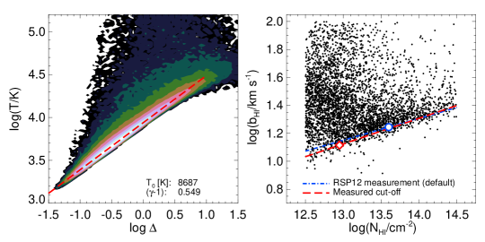
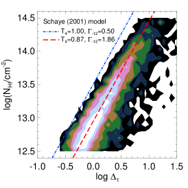
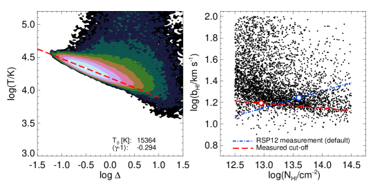
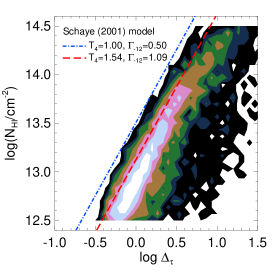
Figure 1: Top left: Contour plot of the volume weighted IGM $T$–$\Delta$ plane in one of the hydrodynamical simulations used in this study. The number density of the data points increases by $0.5$ dex with each contour level. The red dashed line displays the power-law approximation, $T=T_{0}\Delta^{\gamma-1}$, to the $T$–$\Delta$ relation at $\log\Delta\leq 1$. Top middle: The corresponding $b_{\rm HI}$–$N_{\rm HI}$ plane for $4\,000$ absorption features identified in mock Ly$\alpha$ forest spectra drawn from the simulation. The red dashed line corresponds to the measured $b_{\rm HI}$–$N_{\rm HI}$ cut-off, while the blue dot-dashed line shows the observational measurement presented by RSP12. The red diamond indicates the column density corresponding to gas with an optical depth weighted overdensity of $\log\Delta_{\tau}=0$ in the simulation, $N_{\rm HI,0}$, and the blue circle shows the value assumed by RSP12. Top right: Contour plot of $N_{\rm HI}$ against the optical depth weighted gas overdensity at the line centres. The number density of data points increases by $0.25$ dex within each contour level. The red dashed curve displays the analytical model of Schaye (2001), evaluated using the parameters adopted in the simulation. The blue dot-dashed line instead assumes $T_{4}=1$ and $\Gamma_{-12}=0.5$. Bottom: As for the upper panels, but now for a simulation with an inverted $T$–$\Delta$ relation. Note that the blue dot-dashed line in the middle panel again shows the observational measurement from RSP12.

Measurements of the $b_{\rm HI}$–$N_{\rm HI}$ cut-off obtained from two of our hydrodynamical simulations are displayed in Fig. 1. The left-most panels display the $T$–$\Delta$ relation in the simulations. The power-law relationship between the gas at the lower boundary of the $T$–$\Delta$ plane, shown by the red dashed lines, is estimated by finding the mode of the gas temperature in density bins of width 0.02 dex at $\log\Delta=0$ and $-0.75$. The middle panels show the corresponding $b_{\rm HI}$–$N_{\rm HI}$ plane and the measured cut-off (red dashed lines). For comparison, the RSP12 observational measurement is displayed by the blue dot-dashed lines; note this is shown in both of the middle panels and is not a fit to the simulation data. The simulation in the top panels has a maximally steep $T$–$\Delta$ relation with $(\gamma-1)=0.55$, while the bottom panels display a model with an inverted $T$–$\Delta$ relation, $(\gamma-1)=-0.29$. This qualitative comparison indicates that a $T$–$\Delta$ relation which is inverted over $10^{12.5}\leq N_{\rm HI}/[\rm\,cm^{-2}]\leq 10^{14.5}$ is indeed inconsistent with the Voigt profile fits to the KBSS data, in agreement with the conclusion of RSP12. However, the value of $N_{\rm HI,0}$ in the simulations, indicated by the red diamond in the middle panels, is $\sim 0.65$ dex smaller than the value used by RSP12, shown by the blue circle.

The explanation for this becomes apparent on examining the right-most panels in Fig. 1, which display the relationship between $N_{\rm HI}$ and the corresponding optical depth-weighted overdensities at the line centres. The blue dot-dashed lines display Eq. (5) assuming $T_{0,4}=1$ and $\Gamma_{-12}=0.5$. The slope of this relation is in excellent agreement with the simulation data, implying that a power law relationship between $\Delta$ and $N_{\rm HI}$, as inferred by Schaye (2001), is a very good approximation.

On the other hand, the normalisation of this relation disagrees with the simulations. Since the temperature dependence of Eq. (5) is weak, this difference is mainly due to the low value of $\Gamma_{-12}=0.5$ RSP12 used to estimate $N_{\rm HI,0}$. This was based on the results of Faucher-Giguère et al. (2008), who inferred $\Gamma_{-12}$ from the Ly$\alpha$ forest opacity assuming an IGM temperature at mean density of $T_{0}=2.1\times 10^{4}\rm\,K$ (Zaldarriaga et al. 2001). As Faucher-Giguère et al. (2008) correctly point out, the Ly$\alpha$ forest opacity constrains the quantity $T_{0}^{-0.72}/\Gamma_{-12}$, and so assuming a larger (smaller) IGM temperature at mean density will translate their constraint into a smaller (larger) value of $\Gamma_{-12}$ if the Ly$\alpha$ opacity remains fixed. In addition, Faucher-Giguère et al. (2008) obtained their $\Gamma_{-12}$ measurements using an analytical model for IGM absorption which ignored the effect of redshift space distortions on the Ly$\alpha$ forest opacity. Including peculiar velocities and line broadening, as we do with our simulations, raises the $\Gamma_{-12}$ required to match a given value of the mean transmission in the Ly$\alpha$ forest by up to 30 per cent (Becker & Bolton 2013). The Faucher-Giguère et al. (2008) measurements are therefore systematically lower (by a factor of two or more) compared to the value we require to match our mock spectra to the mean transmission measurements of Becker et al. (2013) if $T_{0}\sim 1\times 10^{4}\rm\,K$.

This is demonstrated by the red dashed lines in the right-hand panels of Fig. 1, which display Eq. (5) evaluated using the photo-ionisation rates and gas temperatures used in the simulations. Although the agreement between the analytical model and simulations is still not perfect, the higher $\Gamma_{-12}$ values result in a significantly improved correspondence. We therefore conclude that the value $N_{\rm HI,0}=10^{13.6}\rm\,cm^{-2}$ assumed by RSP12 is biased high by $\sim 0.65$ dex. As we will demonstrate, this bias translates into a significant overestimate of $T_{0}$. Finally, note that the 68 (95) per cent bounds on the range of optical depth weighted overdensities probed by absorption lines with column densities $10^{12.5}\leq N_{\rm HI}/[\rm\,cm^{-2}]\leq 10^{14.5}$ are $-0.2\la\log\Delta_{\tau}\la 0.7$ ($-0.4\la\log\Delta_{\tau}\la 1.2$) at $z=2.4$. The $b_{\rm HI}$–$N_{\rm HI}$ cut-off approach will be largely insensitive to the slope of the $T$–$\Delta$ relation outside this range of overdensities.

3.2 A re-evaluation of the inferred $T$–$\Delta$ relation at $\langle z\rangle=2.37$

We now turn to the key result of this work, summarised in Fig. 2, which displays the relationship between $b_{\rm HI,0}$–$T_{0}$ (upper panel) and $(\gamma-1)$–$(\Gamma-1)$ (lower panel) obtained from the hydrodynamical simulations. Our choice of $N_{\rm HI,0}=10^{12.95}\rm\,cm^{-2}$ corresponds to the average value of $N_{\rm HI}$ associated with gas with $\log\Delta_{\tau}=0$ in all 18 simulations used in the analysis. In practice, $N_{\rm HI,0}$ varies slightly from one simulation to the next due to the weak dependence of the column density on the thermal state of the gas, ranging from $10^{12.8}\rm\,cm^{-2}$ to $10^{13.1}\rm\,cm^{-2}$ in our coldest to hottest simulations. We found adopting values of $N_{\rm HI,0}$ outside of this range introduces an increasingly significant scatter into the $b_{\rm HI,0}$–$T_{0}$ correlation (see also fig. 5 in Schaye et al. 2000), invalidating the assumption that Eq. (4) is a single power-law (i.e. that $\zeta_{1}=0$ holds) and biasing any measurement of $T_{0}$ if $(\gamma-1)\neq 0$.

The dashed red lines in Fig. 2 display the best fit power-laws to the simulation data given by Eqs. (1) and (2), where $\zeta_{2}=1.46$, $\xi_{1}=0.65$ and $\xi_{2}=2.23$ assuming $\zeta_{1}=0$ and $N_{\rm HI,0}=10^{12.95}\rm\,cm^{-2}$. The blue dot-dashed lines display the analytical relations used by RSP12. The dotted lines with shaded error regions show the RSP12 measurements for two value of $N_{\rm HI,0}$. The grey bands correspond to the case where we have rescaled the default RSP12 $b_{\rm HI,0}$ to the value measured at $N_{\rm HI}=10^{12.95}\rm\,cm^{-2}$. The light blue band in the upper panel of Fig. 2 shows their original measurement assuming $N_{\rm HI,0}=10^{13.6}\rm\,cm^{-2}$. The best-fit $b_{\rm HI,0}$–$T_{\rm 0}$ relation lies slightly above the result for pure thermal broadening, indicating that additional processes such as Jeans smoothing (which also scales as $T^{1/2}$, see e.g. Gnedin & Hui 1998) and Hubble broadening impact on the minimum line width.

For comparison, the solid black lines display the relationship at $z=3$ found from the simulations performed by S99. These authors inferred a similar slope for the $b_{\rm HI,0}$–$T_{\rm 0}$ relation, but with a positive offset of around $\sim 0.1\rm\,dex$ relative to this work. Aside from the slightly lower redshift we consider here, there are several possible explanations for this result. The first is the smaller dynamic range of the hydrodynamical simulations used by S99, which employed a gas particle mass of $1.65\times 10^{6}(\Omega_{\rm b}h^{2}/0.0125)(h/0.5)^{-3}M_{\odot}$ within a box size of $2.5h^{-1}\rm\,Mpc$ and were performed with a modified version of the smoothed particle hydrodynamics code HYDRA (Couchman et al. 1995). Additionally, the six simulations S99 analysed all used different assumptions for cosmological parameters and the IGM thermal history, which further complicates a direct comparison. A final possibility is that there are differences in the version of VPFIT S99 used to fit the absorption lines. The results presented by S99 already indicated that the assumption of purely thermal broadening may result in an overestimate of the gas temperature, but our analysis suggests that the factor by which the velocity widths of the lines at the $b_{\rm HI}$–$N_{\rm HI}$ cut-off are actually increased by non-thermal broadening is rather small.

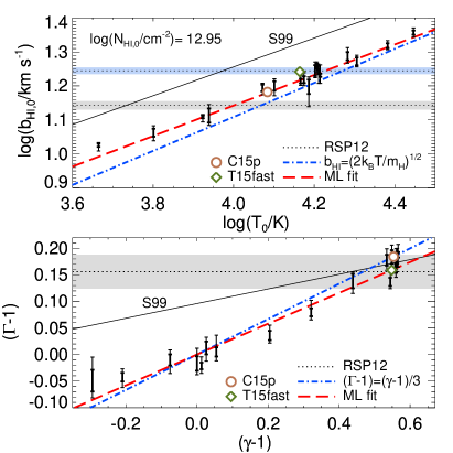
Figure 2: Measurements of the amplitude $b_{\rm HI,0}$ (upper panel) and slope $(\Gamma-1)$ (lower panel) of the $b_{\rm HI}$–$N_{\rm HI}$ cut-off against the corresponding $T_{0}$ and $(\gamma-1)$ from $18$ hydrodynamical simulations. The thick (thin) bootstrap error bars correspond to the 68 (95) per cent confidence intervals around the median. The red dashed lines give the maximum likelihood power-law fits to the data using the bootstrapped uncertainty distributions, while the blue dot-dashed lines display the analytical relations used by RSP12. The solid black lines show the power-law relations S99 inferred from their hydrodynamical simulations (note these are obtained at $z=3$ rather than $z=2.4$), and the grey shaded bands display the RSP12 default measurements. Note that the RSP12 measurement of $b_{\rm HI,0}$ has been rescaled to correspond to $N_{\rm HI,0}=10^{12.95}\rm\,cm^{-2}$; the light blue band gives the value measured by RSP12 when assuming $N_{\rm HI,0}=10^{13.6}\rm\,cm^{-2}$. The models C$15_{\rm P}$ and T15fast refer to two additional simulations which test the effect of cosmological parameters and Jeans smoothing (see text for details). These latter two models were not included in the maximum likelihood fits.

The relatively good agreement of the slopes of the best-fit and analytical relations in Fig. 2 reflects the fact that both Eq. (5) and the assumption that $b_{\rm HI}\propto T^{1/2}$ at the $b_{\rm HI}$–$N_{\rm HI}$ cut-off capture the results of simulations quite accurately. Interestingly, however, although the slope of the $b_{\rm HI}$–$T_{0}$ relation is similar to that found by S99 at $z=3$, we find a much steeper slope for the relationship between $(\Gamma-1)$ and $(\gamma-1)$. S99 concluded the weaker dependence they found between $(\Gamma-1)$ and $(\gamma-1)$ would hamper any precise measurement of the slope of the $T$–$\Delta$ relation. Our results instead suggest that at $z\sim 2.4$ the slope of the $b_{\rm HI}$–$N_{\rm HI}$ cut-off is able to discriminate rather well between differing $T$–$\Delta$ relations. We have checked that using the smaller line sample (300 lines, with 500 bootstrap resamples) used by S99 increases the uncertainties on the cut-off measurements but does not change this conclusion. The exact explanation for this difference is again unclear, although we again speculate differences in the hydrodynamical simulations may play a role. However, the potentially greater sensitivity to $(\gamma-1)$ provides additional motivation for revisiting $b_{\rm HI}$–$N_{\rm HI}$ cut-off measurements at higher redshifts.

We have also verified that the best-fit power-law relations in Fig. 2 should be robust to small differences in the assumed cosmology and uncertainties in the pressure (Jeans) smoothing scale of gas in the IGM (see Rorai et al. 2013 for a recent discussion). The circles show $b_{\rm HI,0}$ and $(\Gamma-1)$ measured from an additional simulation, C15_P (see Becker & Bolton 2013), which was performed with cosmological parameters consistent with the Planck results, $\Omega_{\rm m}=0.308$, $\Omega_{\Lambda}=0.692$, $\Omega_{\rm b}h^{2}=0.0222$, $h=0.678$, $\sigma_{8}=0.829$ and $n_{\rm s}=0.961$ (Planck Collaboration XVI 2013). The diamonds show the results obtained from the simulation T15fast described in Becker et al. (2011). This simulation rapidly heats the IGM from $z=3.5$–$3.0$ by $\sim 9\,000\rm\,K$, in contrast to the more gradual heating used in our fiducial simulations. The good agreement of both these models with the best-fit relations indicates that neither of these issues should be a significant concern in our analysis.

Combining these results with Eqs. (3)–(4) and applying them to the default RSP12 measurement of $b_{\rm HI,0}$ and $(\Gamma-1)$, we infer $T_{0}=[1.00^{+0.32}_{-0.21}]\times 10^{4}\rm\,K$ and $(\gamma-1)=0.54\pm 0.11$ at $\langle z\rangle=2.37$ (cf. $T_{0}=[1.87\pm 0.08]\times 10^{4}\rm\,K$ and $\gamma-1=0.47\pm 0.10$ from RSP12). Note that we do not recompute the RSP12 statistical uncertainty estimates; we instead simply rescale their published measurements of $b_{\rm HI,0}$ and $(\Gamma-1)$ using the results of our simulations. We have, however, added (in quadrature) an additional systematic error to our measurement of $T_{0}$ by assuming an uncertainty of $\pm 0.2$ dex in $\log\Delta$, the fractional overdensity corresponding to the column density $N_{\rm HI,0}$ at which $T_{0}$ is measured (i.e. $\log\Delta=0.0\pm 0.2$). This accounts for the intrinsic scatter in the relationship between $N_{\rm HI}$ and $\Delta_{\tau}$ in our simulations (see Fig. 1) as well as the small uncertainty in the mean transmitted flux in the Ly$\alpha$ forest (Becker et al. 2013).

Our recalibrated measurement for the slope of the $T$–$\Delta$ relation is fully consistent with RSP12. Importantly, however, we find their measurement of $T_{0}$ is biased high by around $9\,000\rm\,K$. This is primarily due the value of $N_{\rm HI,0}=10^{13.6}\rm\,cm^{-2}$ they adopt in their analysis – this column density corresponds to gas with $\Delta\sim 2$–$4$ in our simulations – and to a smaller extent their assumption of pure thermal broadening at the $b_{\rm HI}$–$N_{\rm HI}$ cut-off. Finally, we stress we did not reanalyse the RSP12 observational data in this work. As a result we are unable to fully assess the importance of other potential systematics such as metal line contamination, spurious line fits or bias due to differences in the line fitting procedure (e.g. Rauch et al. 1993). Ideally, potential biases arsing from the latter two possibilities should be minimised by applying exactly the same line profile fitting procedure to both the observations and simulations (e.g. S99, Bolton et al. 2012).

3.3 Comparison to previous measurements

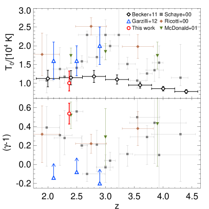
Figure 3: A comparison of the temperature at mean density, $T_{0}$ (top panel), and slope of the $T$–$\Delta$ relation, $(\gamma-1)$ (bottom panel), inferred in this work (red circles) to other recent constraints obtained using a variety of different methods at $2\leq z\leq 4.5$. These are: the curvature statistic from Becker et al. (2011) (black diamonds); the wavelet amplitude PDF from Garzilli et al. (2012) (blue triangles), and the $b_{\rm HI}$–$N_{\rm HI}$ cut-off analyses presented by Schaye et al. (2000) (grey squares), Ricotti et al. (2000) (orange diamonds) and McDonald et al. (2001) (inverted green triangles). All uncertainties are 1$\sigma$. The $T_{0}$ values inferred from the measurements of Becker et al. (2011) assume $(\gamma-1)=0.54\pm 0.11$, i.e. the value inferred in this work at $z=2.4$.

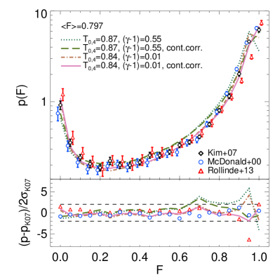
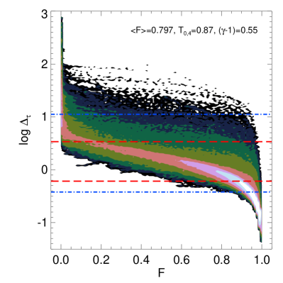
Figure 4: Top left: The probability distribution of the transmitted flux (PDF) at $z\sim 2.5$. The observational data are from K07 at $\langle z\rangle=2.52$, Rollinde et al. (2013) at $\langle z\rangle=2.5$ and McDonald et al. (2000) at $\langle z\rangle=2.4$. The data points from the latter two studies have been offset by $\Delta F=\pm 0.0125$ for clarity of presentation. The curves display the PDF obtained from two different hydrodynamical simulations of the Ly$\alpha$ forest at $z=2.553$ which assume a $T$–$\Delta$ relation with either $(\gamma-1)=0.55$ or $(\gamma-1)=0.01$. Each of these models is furthermore shown with and without an estimate for the continuum correction (see text for details). Bottom left: The difference between the mock data and observations from Rollinde et al. (2013) and McDonald et al. (2000) with respect to K07, normalised by twice the 1$\sigma$ K07 jack-knife errors. This accounts for a possible factor of two underestimate in the sample variance suggested by Rollinde et al. (2013). The horizontal dashed lines display the 2$\sigma$ bound for these increased error estimates. Right: Contour plot of the optical depth weighted overdensity against the transmitted flux in each pixel of the mock spectra drawn from the simulation with $T_{0,4}=0.87$ and $(\gamma-1)=0.55$. The number density of pixels increases by $0.5$ dex within each contour level. The horizontal red dashed (blue dot-dashed) lines bound 68 (95) per cent of the overdensities corresponding to absorption lines with $10^{12.5}\leq N_{\rm HI}/[{\rm cm^{-2}}]\leq 10^{14.5}$.

Our recalibrated measurements of the $T$–$\Delta$ relation at $z\sim 2.4$ are compared to previous measurements in Fig. 3. The $T_{0}$ and $(\gamma-1)$ constraints obtained in this study are in excellent agreement with the recent, independent measurement presented by Becker et al. (2011) using the curvature statistic. These authors directly measure $T(\bar{\Delta})=[2.54\pm 0.13]\times 10^{4}\rm\,K$ ($2\sigma$) at a characteristic overdensity of $\bar{\Delta}=4.4$ at $z=2.4$. The $T_{0}$ and $(\gamma-1)$ results rederived here from the RSP12 data translate to a value of $T(\bar{\Delta})=[2.22^{+0.80}_{-0.59}]\times 10^{4}\rm\,K$ (1$\sigma$), which is fully consistent with the Becker et al. (2011) value. Alternatively, translating the Becker et al. (2011) $T(\bar{\Delta})$ measurement to a temperature at the mean density assuming $(\gamma-1)=0.54\pm 0.11$ yields $T_{0}=[1.15\pm 0.19]\times 10^{4}\rm\,K$ ($1\sigma$). For the value of $(\gamma-1)$ measured here, therefore, both the Becker et al. (2011) measurements and the present results are consistent with a value of $T_{0}$ near $1\times 10^{4}\rm\,K$ at $z=2.4$. Note that Becker et al. (2011) also strongly constrain $T_{0}$ to be relatively low at $z>4$, where the characteristic overdensity probed by the curvature approaches the mean density. For example, at $z=4.4$ they find $T_{0}$ to be in the range 0.70–0.94 $\times 10^{4}\rm\,K$ (2$\sigma$) for $(\gamma-1)=$ 1.3–1.5. This implies only a moderate boost to the IGM temperature at mean density during He$\,\rm\scriptstyle II\$reionisation, although the precise evolution of $T_{0}$ over $2.4<z<4.4$ will depend on the evolution of $(\gamma-1)$ over these redshifts.

Our measurement of $T_{0}$ is also in reasonable agreement with those of Garzilli et al. (2012), who performed an analysis of the wavelet amplitude PDF (see also Lidz et al. 2010), obtaining $T_{0}=[1.6\pm 0.4]\times 10^{4}\rm\,K$ ($1\sigma$) at the slightly higher redshift of $z=2.5$. We are also consistent with the earlier $b_{\rm HI}$–$N_{\rm HI}$ measurements obtained by Schaye et al. (2000) at $z=2.4$; as already discussed these authors used a similar technique but smaller data set compared to RSP12. We are unable to directly compare the $b_{\rm HI}$–$N_{\rm HI}$ measurements from Ricotti et al. (2000) to our measurement, since these authors do not present results at $z=2.4$. However, they find a signficantly larger value of $T_{0}=25200\pm 2300\rm\,K$ at $z=2.75$, which would require a $T$–$\Delta$ relation slope of $(\gamma-1)\sim 1$ for consistency with the Becker et al. (2011) measurements at the same redshift. Finally, McDonald et al. (2001), again using the $b_{\rm HI}$–$N_{\rm HI}$ cut-off (although with a different method to Schaye et al. 2000), infer $T=2.26\pm 0.19\times 10^{4}\rm\,K$ at $\Delta=1.66\pm 0.11$. Although these authors do not present a measurement of $T_{0}$, using their measurement of $(\gamma-1)=0.52\pm 0.14$ this corresponds to $T_{0}=1.74\pm 0.20\times 10^{4}\rm\,K$. This temperature is somewhat higher than the three other measurements at $z=2.4$, by $2$–$3\sigma$. Despite this, however, there appears to be a reasonable consensus on the thermal state of the low-density IGM at $z\sim 2.4$ from both Ly$\alpha$ transmission statistics and line decomposition analyses.

On the other hand, while our revised value of $(\gamma-1)=0.54\pm 0.11$ is fully consistent with the original line decomposition analyses of Schaye et al. (2000) and McDonald et al. (2001) and the lower limits from the wavelet PDF obtained by Garzilli et al. (2012), as noted by RSP12 there appears to be some tension with constraints based on the observed transmission PDF (Kim et al. 2007, hereafter K07) which appear to favour an isothermal or perhaps even inverted $T$–$\Delta$ relation at $2<z<3$ (Bolton et al. 2008; Viel et al. 2009). In the left hand panel of Fig. 4 we revisit this by comparing the PDF of the transmitted flux from two of our hydrodynamical simulations to three observational measurements of the Ly$\alpha$ forest transmission PDF from high resolution ($R\sim 40\,000$) data at $z\simeq 2.4$–$2.5$ (K07, McDonald et al. 2000; Rollinde et al. 2013). The mock spectra have been drawn from models with a $T$–$\Delta$ relation with either $(\gamma-1)=0.55$ or $(\gamma-1)=0.01$ at $z=2.553$, and have a $T_{0}$ value close to the revised measurement obtained in this work. The spectra have been processed following a similar procedure to that outlined in Section 2.1, with two key differences. Firstly, the spectra are scaled to match the mean transmission of the K07 PDF data, $\langle F\rangle=0.797$ at $\langle z\rangle=2.52$, and Gaussian distributed noise matching the variances, $\sigma_{\rm F}$, in each bin of the K07 PDF is added. Secondly, for each model we also implement an iterative continuum correction to the spectra to mimic the effect of a possible continuum placement error on the K07 data. We first compute the median transmitted flux in each of our mock sight-lines and then deselect all pixels below $1\sigma_{\rm F}$ of this value. This procedure is then repeated for the remaining pixels until convergence is achieved. The final median flux is selected as the new continuum level.

The comparison in Fig. 4 demonstrates a $T$–$\Delta$ relation with $(\gamma-1)=0.55$ is inconsistent with the K07 data at $4$–$7\sigma$ at $0.6<F<0.8$, even when accounting for possible continuum misplacement (although see the analysis presented by Lee 2012 using an analytical model for the transmission PDF). An isothermal model on the other hand is in within $1$–$3\sigma$ of the K07 data over the same interval. This is fully consistent with the more detailed analysis performed by Viel et al. (2009) and Bolton et al. (2008). Note, however, that Rollinde et al. (2013) recently argued that the error bars quoted on the K07 PDF measurements may be larger by up to a factor of two simply due to sample variance; these authors demonstrated the bootstrap or jack-knife errors on the data will be underestimated if the chunk size which the spectra are sampled over is too small. Comparison of the three observational measurements in Fig. 4 likewise suggests that the errors on the PDF measurements have been initially underestimated.

The lower panel in Fig. 4 therefore displays the difference between the K07 PDF and the mock data and observations from Rollinde et al. (2013) and McDonald et al. (2000), divided through by twice the 1$\sigma$ jack-knife errors reported by K07. With these larger uncertainties the discrepancy with the $(\gamma-1)=0.55$ model decreases, although the difference between the simulation and data is still $\sim 2$–$3\sigma$ at $0.6<F<0.8$ after accounting for a plausible continuum placement error. This is in reasonable agreement with Rollinde et al. (2013), who also reproduce the K07 PDF at $z=2.5$ to within 2–3$\sigma$ of the expected dispersion estimated from mock spectra drawn from the GIMIC simulation suite (Crain et al. 2009) assuming $(\gamma-1)\sim 0.35$ and $\langle F\rangle=0.770$. Rollinde et al. (2013) conclude there is no evidence for a significant departure from a power-law $T$–$\Delta$ relation with $(\gamma-1)>0$. The remaining disagreement between the observations and a model with $(\gamma-1)=0.55$ suggests that increased errors due to continuum placement and sample variance may still not fully account for the true uncertainties on the observational data.

In this context, it is worth stressing that the transmission PDF and $b_{\rm HI}$–$N_{\rm HI}$ cut-off are sensitive to a different range of IGM gas densities and hence also temperatures. The right-hand panel of Fig. 4 displays the relationship between the optical depth weighted overdensity and transmitted flux in each pixel of the spectra drawn from the simulation with $(\gamma-1)=0.55$, shown in the left panel. For comparison, the red dashed (blue dot-dashed) lines bound 68 (95) per cent of the overdensities probed corresponding to absorption lines with $10^{12.5}\leq N_{\rm HI}/[{\rm cm^{-2}}]\leq 10^{14.5}$ (i.e. the range used to measure the $b_{\rm HI}$–$N_{\rm HI}$ cut-off at $z\sim 2.4$). Interestingly, the largest differences between models and observations of the PDF arise almost exclusively in the underdense regions which are not well sampled by the $b_{\rm HI}$–$N_{\rm HI}$ cut-off measurements. Furthermore, note that the $b_{\rm HI}$–$N_{\rm HI}$ cut-off is only sensitive to the coldest gas lying along the lower bound of the $T$–$\Delta$ plane (e.g. S99). It therefore remains possible that a more complicated, multiple valued $T$–$\Delta$ plane with significant scatter and/or a separate hot IGM component confined to the most underdense regions, $\log\Delta_{\tau}\sim-0.5$, may also influence the shape of the PDF at $F>0.7$. Indeed, recent radiative transfer simulations of He$\,\rm\scriptstyle II\$reionisation predict significant scatter or even bimodality in the $T$–$\Delta$ plane at $z\sim 3$ (Meiksin & Tittley 2012; Compostella et al. 2013). More detailed studies of both the PDF and the $b_{\rm HI}$–$N_{\rm HI}$ distribution over a wider redshift range, combined with simulations which have increased dynamic range and/or incorporate radiative transfer effects, will therefore be required to establish the importance of these effects.

4 Conclusions

We have performed a careful calibration of the measurement of the $T$–$\Delta$ relation in the low-density IGM at $z\sim 2.4$. Our analysis is based on the $b_{\rm HI}$–$N_{\rm HI}$ cut-off measured from mock Ly$\alpha$ forest spectra drawn from an extensive set of high-resolution hydrodynamical simulations, combined with accurate measurements of the mean transmitted flux in the Ly$\alpha$ forest (Becker et al. 2013) and the KBSS line profile fits from RSP12. We confirm the high value of the power-law slope, $(\gamma-1)$, at $z\sim 2.4$ advocated by RSP12, but we find a value for the temperature at mean density, $T_{0}$, which is smaller by almost a factor of two. The latter is mainly due to a difference of $0.65$ dex in the calibration of the $N_{\rm HI}$–$\Delta$ correlation. The lower inferred value for the temperature brings the measurement of RSP12 into excellent agreement with the Becker et al. (2011) constraint on the IGM temperature at the same redshift, but inferred at somewhat higher gas density using the curvature distribution of the transmitted flux. More generally, recent IGM temperature measurements appear to now show reasonable agreement and to favour the lower end of the range of previously discussed values, suggesting that the heat injection into the IGM during He$\,\rm\scriptstyle II\$reionisation was moderate.

However, the high value of $(\gamma-1)$ which now appears to have been measured with reasonable accuracy from the $b_{\rm HI}$–$N_{\rm HI}$ distribution at $z\sim 2.4$ disagrees with that inferred from the transmitted flux PDF at $z\sim 2.5$ (at 2–3$\sigma$ for $0.6<F<0.8$) even if assuming (i) previously reported uncertainties on the PDF have been underestimated by a factor of two and (ii) a plausible estimate for the continuum placement uncertainty (see also Lee 2012; Rollinde et al. 2013). While it is possible this difference is due to systematic uncertainties which remain underestimated, it is important to emphasise that the $b_{\rm HI}$–$N_{\rm HI}$ distribution and PDF are sensitive to the temperature of the IGM in nearly disjunct density ranges, with the PDF largely probing densities below the mean. While it appears very likely the IGM $T$–$\Delta$ relation is not inverted during He$\,\rm\scriptstyle II\$reionisation from both an observational and theoretical perspective (e.g. McQuinn et al. 2009; Bolton et al. 2009), it may be too early to completely discard the interesting possibility that our understanding of the heating of the highly underdense IGM is still incomplete.

The convergence towards a self-consistent set of parameters describing the $T$–$\Delta$ relation at $z\simeq 2.4$ represents an encouraging step towards establishing the detailed thermal history of the high-redshift IGM. The extension of the measurements based on the $b_{\rm HI}$–$N_{\rm HI}$ distribution to a wider redshift range, and the development of methods that can push the temperature measurements to lower density and search for the predicted scatter or even bimodality in the $T$–$\Delta$ plane during He$\,\rm\scriptstyle II\$reionisation (e.g. Meiksin & Tittley 2012; Compostella et al. 2013) will hopefully lead to a fuller characterisation of the thermal state of the IGM and its evolution, and thus more generally to the properties of ionising sources in the early Universe.

Appendix A Convergence test

In Fig. 5 we present a convergence test of our results by applying the $b_{\rm HI}$–$N_{\rm HI}$ cut-off algorithm to five simulations with different box sizes and gas particle masses. One of the simulations corresponds to the fiducial box size ($10h^{-1}\rm\,Mpc$) and gas particle mass resolution ($M_{\rm gas}=9.2\times 10^{4}h^{-1}M_{\odot}$) used in this work. Two further models test the mass resolution within a $10h^{-1}\rm\,Mpc$ box, assuming $M_{\rm gas}=7.4\times 10^{5}h^{-1}M_{\odot}$ and $5.9\times 10^{6}h^{-1}M_{\odot}$, respectively. The final two models test convergence with simulation volume, and have a fixed gas particle mass of $M_{\rm gas}=5.9\times 10^{6}h^{-1}M_{\odot}$ within $20h^{-1}\rm\,Mpc$ and $40h^{-1}\rm\,Mpc$ boxes. These five simulations are also described in Becker et al. (2011), and correspond to models C15 and R1–R4 in their table 2.

Mock spectra extracted at $z=2.355$ were analysed using the procedure described in Section 2 using a sample of $4\,000$ lines, with uncertainties on $b_{\rm HI,0}$ and $(\Gamma-1)$ estimated by bootstrap sampling with replacement $4\,000$ times. The measurements of $b_{\rm HI,0}$ and $(\Gamma-1)$ are consistent within the 68 per cent bootstrapped confidence intervals around the median, indicating that our results should be well converged with box size and mass resolution. We have further verified that a smaller sample of 300 lines (e.g. S99) significantly increases the bootstrapped uncertainties but does not introduce a systematic offset to the results.

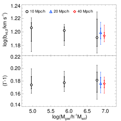
Figure 5: The amplitude, $b_{\rm HI,0}$ (top panel), and slope, $(\Gamma-1)$ (bottom panel) of the $b_{\rm HI}$–$N_{\rm HI}$ cut-off measured from simulations with either a fixed box size ($10h^{-1}\rm\,Mpc$, black circles) or fixed mass resolution ($M_{\rm gas}=5.9\times 10^{6}h^{-1}M_{\odot}$) using a sample of $4\,000$ Ly$\alpha$ absorption lines. For clarity of presentation the blue triangles and red diamonds have been offset in $\log M_{\rm gas}$ by $0.1$ and $0.2$ dex, respectively. The thick (thin) bootstrap error bars correspond to the 68 (95) per cent confidence intervals around the median. The fiducial box size and mass resolution used in this work are $10h^{-1}\rm\,Mpc$ and $M_{\rm gas}=9.2\times 10^{4}h^{-1}M_{\odot}$.

References

- Becker & Bolton (2013) Becker, G. D. & Bolton, J. S. 2013, MNRAS in press, arXiv:1307.2259
- Becker et al. (2011) Becker, G. D., Bolton, J. S., Haehnelt, M. G., & Sargent, W. L. W. 2011, MNRAS, 410, 1096
- Becker et al. (2013) Becker, G. D., Hewett, P. C., Worseck, G., & Prochaska, J. X. 2013, MNRAS, 430, 2067
- Bolton et al. (2004) Bolton, J., Meiksin, A., & White, M. 2004, MNRAS, 348, L43
- Bolton et al. (2012) Bolton, J. S., Becker, G. D., Raskutti, S., Wyithe, J. S. B., Haehnelt, M. G., & Sargent, W. L. W. 2012, MNRAS, 419, 2880
- Bolton et al. (2010) Bolton, J. S., Becker, G. D., Wyithe, J. S. B., Haehnelt, M. G., & Sargent, W. L. W. 2010, MNRAS, 406, 612
- Bolton et al. (2009) Bolton, J. S., Oh, S. P., & Furlanetto, S. R. 2009, MNRAS, 395, 736
- Bolton et al. (2008) Bolton, J. S., Viel, M., Kim, T.-S., Haehnelt, M. G., & Carswell, R. F. 2008, MNRAS, 386, 1131
- Bryan & Machacek (2000) Bryan, G. L. & Machacek, M. E. 2000, ApJ, 534, 57
- Cen et al. (2009) Cen, R., McDonald, P., Trac, H., & Loeb, A. 2009, ApJ, 706, L164
- Compostella et al. (2013) Compostella, M., Cantalupo, S., & Porciani, C. 2013, MNRAS, 435, 3169
- Couchman et al. (1995) Couchman, H. M. P., Thomas, P. A., & Pearce, F. R. 1995, ApJ, 452, 797
- Crain et al. (2009) Crain, R. A. et al., 2009, MNRAS, 399, 1773
- Faucher-Giguère et al. (2008) Faucher-Giguère, C.-A., Lidz, A., Hernquist, L., & Zaldarriaga, M. 2008, ApJ, 688, 85
- Furlanetto & Oh (2009) Furlanetto, S. R. & Oh, S. P. 2009, ApJ, 701, 94
- Garzilli et al. (2012) Garzilli, A., Bolton, J. S., Kim, T.-S., Leach, S., & Viel, M. 2012, MNRAS, 424, 1723
- Gnedin & Hui (1998) Gnedin, N. Y. & Hui, L. 1998, MNRAS, 296, 44
- Green (2011) Green, D. A. 2011, Bulletin of the Astronomical Society of India, 39, 289
- Haehnelt & Steinmetz (1998) Haehnelt, M. G. & Steinmetz, M. 1998, MNRAS, 298, L21
- Hui & Gnedin (1997) Hui, L. & Gnedin, N. Y. 1997, MNRAS, 292, 27
- Hui & Haiman (2003) Hui, L. & Haiman, Z. 2003, ApJ, 596, 9
- Kim et al. (2007) Kim, T.-S., Bolton, J. S., Viel, M., Haehnelt, M. G., & Carswell, R. F. 2007, MNRAS, 382, 1657 (K07)
- Lee (2012) Lee, K.-G. 2012, ApJ, 753, 136
- Lidz et al. (2010) Lidz, A., Faucher-Giguère, C.-A., Dall’Aglio, A., McQuinn, M., Fechner, C., Zaldarriaga, M., Hernquist, L., & Dutta, S. 2010, ApJ, 718, 199
- McDonald et al. (2001) McDonald, P., Miralda-Escudé, J., Rauch, M., Sargent, W. L. W., Barlow, T. A., & Cen, R. 2001, ApJ, 562, 52
- McDonald et al. (2000) McDonald, P., Miralda-Escudé, J., Rauch, M., Sargent, W. L. W., Barlow, T. A., Cen, R., & Ostriker, J. P. 2000, ApJ, 543, 1
- McQuinn et al. (2009) McQuinn, M., Lidz, A., Zaldarriaga, M., Hernquist, L., Hopkins, P. F., Dutta, S., & Faucher-Giguère, C.-A. 2009, ApJ, 694, 842
- Meiksin & Tittley (2012) Meiksin, A. & Tittley, E. R. 2012, MNRAS, 423, 7
- Miniati & Elyiv (2013) Miniati, F. & Elyiv, A. 2013, ApJ, 770, 54
- Miralda-Escudé & Rees (1994) Miralda-Escudé, J. & Rees, M. J. 1994, MNRAS, 266, 343
- Planck Collaboration XVI (2013) Planck Collaboration XVI, 2013, A&A submitted, arXiv:1303.5076
- Puchwein et al. (2012) Puchwein, E., Pfrommer, C., Springel, V., Broderick, A. E., & Chang, P. 2012, MNRAS, 423, 149
- Raskutti et al. (2012) Raskutti, S., Bolton, J. S., Wyithe, J. S. B., & Becker, G. D. 2012, MNRAS, 421, 1969
- Rauch et al. (1993) Rauch, M., Carswell, R. F., Webb, J. K., & Weymann, R. J. 1993, MNRAS, 260, 589
- Ricotti et al. (2000) Ricotti, M., Gnedin, N. Y., & Shull, J. M. 2000, ApJ, 534, 41
- Rollinde et al. (2013) Rollinde, E., Theuns, T., Schaye, J., Pâris, I., & Petitjean, P. 2013, MNRAS, 428, 540
- Rorai et al. (2013) Rorai, A., Hennawi, J. F., & White, M. 2013, ApJ, 775, 81
- Rudie et al. (2012a) Rudie, G. C., Steidel, C. C., & Pettini, M. 2012a, ApJ, 757, L30 (RSP12)
- Rudie et al. (2012b) Rudie, G. C. et al. 2012b, ApJ, 750, 67
- Schaye (2001) Schaye, J. 2001, ApJ, 559, 507
- Schaye et al. (1999) Schaye, J., Theuns, T., Leonard, A., & Efstathiou, G. 1999, MNRAS, 310, 57 (S99)
- Schaye et al. (2000) Schaye, J., Theuns, T., Rauch, M., Efstathiou, G., & Sargent, W. L. W. 2000, MNRAS, 318, 817
- Shull et al. (2010) Shull, J. M., France, K., Danforth, C. W., Smith, B., & Tumlinson, J. 2010, ApJ, 722, 1312
- Springel (2005) Springel, V. 2005, MNRAS, 364, 1105
- Syphers et al. (2011) Syphers, D., Anderson, S. F., Zheng, W., Meiksin, A., Haggard, D., Schneider, D. P., & York, D. G. 2011, ApJ, 726, 111
- Theuns et al. (1998) Theuns, T., Leonard, A., Efstathiou, G., Pearce, F. R., & Thomas, P. A. 1998, MNRAS, 301, 478
- Theuns et al. (2002a) Theuns, T., Schaye, J., Zaroubi, S., Kim, T., Tzanavaris, P., & Carswell, B. 2002a, ApJ, 567, L103
- Theuns et al. (2002b) Theuns, T., Zaroubi, S., Kim, T.-S., Tzanavaris, P., & Carswell, R. F. 2002b, MNRAS, 332, 367
- Viel et al. (2009) Viel, M., Bolton, J. S., & Haehnelt, M. G. 2009, MNRAS, 399, L39
- Worseck et al. (2011) Worseck, G. et al., 2011, ApJ, 733, L24
- Zaldarriaga et al. (2001) Zaldarriaga, M., Hui, L., & Tegmark, M. 2001, ApJ, 557, 519