The gravitational drag force on an extended object moving in a gas

Abstract

Using axisymmetrical numerical simulations, we revisit the gravitational drag felt by a gravitational Plummer sphere with mass $M$ and core radius $R_{s}$, moving at constant velocity $V_{0}$ through a background homogeneous medium of adiabatic gas. Since the potential is non-diverging, there is no gas removal due to accretion. When $R_{s}$ is larger than the Bondi radius $R_{B}$, the perturbation is linear at every point and the drag force is well fitted by the time-dependent Ostriker’s formula with $r_{\rm min}=2.25R_{s}$, where $r_{\rm min}$ is the minimum impact parameter in the Coulomb logarithm. In the deep nonlinear supersonic regime ($R_{s}\ll R_{B}$), the minimum radius is no longer related with $R_{s}$ but with $R_{B}$. We find $r_{\rm min}=3.3\mathcal{M}^{-2.5}R_{B}$, for Mach numbers of the perturber between $1.5$ and $4$, although $r_{\rm min}=2\mathcal{M}^{-2}R_{B}=2GM/V^{2}_{0}$ also provides a good fit at $\mathcal{M}>2$. As a consequence, the drag force does not depend sensitively on the nonlinearity parameter $\mathcal{A}$, defined as $R_{B}/R_{s}$, for $\mathcal{A}$-values larger than a certain critical value $\mathcal{A}_{\rm cr}$. We show that our generalized Ostriker’s formula for the drag force is more accurate than the formula suggested by Kim & Kim (2009).

1. Introduction

A gravitational perturber moving through a gaseous background creates a density wake in the medium. The complexity of the wake has motivated a number of groups to tackle the problem using numerical simulations (e.g., Hunt 1971, 1979; Shima et al. 1985; Ruffert 1994, 1996; Sánchez-Salcedo & Brandenburg 2001; Cantó et al. 2011, 2012). The gravitating object induces small disturbances in the far-field ambient medium (i.e. in streamlines with large impact parameters) and, consequently, the far-field density structure of the wake can be derived in linear perturbation theory (Dokuchaev 1964; Ruderman & Spiegel 1971). Using this approach, Ostriker (1999) derived the density wake behind a gravitational body of mass $M$ moving at velocity $V_{0}$ on a straight-line trajectory through a homogeneous infinite medium with unperturbed density $\rho_{\infty}$ and sound speed $c_{\infty}$, when the perturber is dropped at $t=0$. For subsonic perturbers, the isodensity contours are closed ellipsoids, which do not contribute to the drag force, except in the outer parts of the wake where the ellipsoids are not closed. Supersonic perturbers generate a density wake only within the rear Mach cone.

Here, we are interested in the dynamical friction, that is, the drag force onto the perturber due to the gravitational interaction with its own induced wake. Thus, once the density of the wake is known, the drag force $F_{DF}$ can be computed as the gravitational force between the perturber and its wake. The drag force is usually written as

$$F_{DF}=\frac{4\pi\rho_{\infty}(GM)^{2}}{V_{0}^{2}}\ln\Lambda,$$ (1)

where $\ln\Lambda$ is the Coulomb logarithm. For subsonic perturbers, i.e. $\mathcal{M}\equiv V_{0}/c_{\infty}<1$, Ostriker (1999) found that, at times satisfying $c_{\infty}t>r_{\rm min}/(1-\mathcal{M})$, the Coulomb logarithm is

$$\ln\Lambda=\frac{1}{2}\ln\left(\frac{1+\mathcal{M}}{1-\mathcal{M}}\right)-\mathcal{M},$$ (2)

where $r_{\rm min}$ is the minimum radius of the effective gravitational interaction of a perturber with the gas. In practice, for a point mass object, $r_{\rm min}$ is taken as the radius at which the linear approximation breaks down. For supersonic perturbers, the Coulomb logarithm is given by

$$\ln\Lambda=\frac{1}{2}\ln\left(1-\mathcal{M}^{-2}\right)+\ln\left(\frac{\mathcal{M}c_{\infty}t}{r_{\rm min}}\right),$$ (3)

for $\mathcal{M}>1$ and $c_{\infty}t>r_{\rm min}/(\mathcal{M}-1)$ (Ostriker 1999).

Sánchez-Salcedo & Brandenburg (1999) tested numerically Ostriker’s formula when the perturber is extended. This could represent a globular cluster orbiting in the gaseous halo of its host galaxy, a young massive star cluster in a merging system, an elliptical galaxy depleted of gas in the intracluster medium, or a galaxy cluster in a major merger environment (e.g., Naiman et al. 2011). Sánchez-Salcedo & Brandenburg (1999) found that Ostriker’s formula describes successfully the temporal evolution and magnitude of the force experienced by a Plummer perturber, when its mass $M$ is small enough so that the gas response to the perturbation is linear. For supersonic perturbers, they inferred $r_{\rm min}=2.25R_{s}$, where $R_{s}$ is the core radius.

Kim & Kim (2009, hereafter KK09) carried out axisymmetric numerical simulations to study the flow past a Plummer sphere in the linear and in the nonlinear regimes. For the linear supersonic regime, they found that the minimum radius in Eq. (3) depends slightly on the Mach number: $r_{\rm min}=0.35{\mathcal{M}}^{0.6}R_{s}$. Moreover, they found in their simulations that the drag force is highly suppressed in the nonlinear regime as compared to the linear case.

In this paper, we revisit the drag force on an extended (non-accreting) gravitating object with a range of velocities relative to the ambient medium. Our aim is to provide a physically more motivated and more accurate formula for the drag force in both the linear and nonlinear cases. In Section 2, we briefly recapitulate the relevant scales in the problem, discuss the ambiguity in the definition of the minimum radius and describe the numerical code adopted in this paper. Section 3 is devoted to discuss the drag force in the linear case. The results for nonlinear simulations are analyzed in Section 4. Finally, we summarize our findings in Section 5.

2. Dynamical friction in a gas: Relevant scales, the minimum cut-off distance and the inner boundary condition

Consider the flow pattern past a gravitational object. The inner structure of the wake (in the vicinity of the object) depends on the adopted equation of state for the gas (e.g., $\gamma$, if the gas behaves as a polytrope, $P\propto\rho^{\gamma}$) and depends also on whether the perturber is a point mass gravitational potential or a non-point mass distribution (e.g., Naiman et al. 2011). As a consequence, the drag force may depend on $\gamma$ and on the adopted inner conditions. For instance, Lee & Stahler (2011) found that, for subsonic perturbers with $\mathcal{M}<0.75$, the drag force felt by a point mass (accretor) is higher than what Ostriker’s formula predicts for extended non-accretors. For hypersonic perturbers, however, Cantó et al. (2011) argued that the drag force expressions (1) and (3), are still valid for a point mass accretor, provided that $r_{\rm min}$ is chosen appropriately. Cantó et al. (2011) demonstrated that $r_{\rm min}\simeq 0.8GM/V_{0}^{2}$ for a hypersonic point mass.

Figure 1.— Cuts along the symmetry axis of the perturbed density $\alpha\equiv(\rho-\rho_{\infty})/\rho_{\infty}$ (upper panel) and of the magnitude $\alpha\partial\Phi_{\rm ext}/\partial z$ in units of $GM/R_{B}^{2}$ (lower panel), using linear theory, for a perturber of mass $M$ traveling at Mach $2$. To compute $\alpha$, we consider two cases for the pertuber: a point-mass perturber (dashed line) and a spherical perturber of constant density with a radius $a=R_{B}$ (solid line). In order to illustrate the error made when Equation (7) is used instead of Equation (6), we plot the term $\alpha\partial\Phi_{\rm ext}/\partial z$, which appears in the integrand of these equations, where $\Phi_{\rm ext}$ represents the gravitational potential created by a homogeneous sphere of radius $R_{B}$.

For a non-point mass perturber, there are three independent characteristic radii in the problem: the softening length $R_{s}$, the Bondi radius $R_{B}\equiv GM/c_{\infty}^{2}$ and the gravitational radius or the so-called accretion radius $R_{A}\equiv 2GM/(c_{\infty}^{2}+V_{0}^{2})=2R_{B}/(1+{\mathcal{M}}^{2})$. On dimensional grounds, one expects that the minimum radius $r_{\rm min}$ in Equation (3) may be expressed as a certain combination of the three characteristic radii.

The linear analysis is expected to provide a good estimate of the drag force in circumstances where the depth of the external gravitational potential $\Phi_{\rm ext}(0)$ is small as compared to $c_{\infty}^{2}$, so that the disturbances are small at any location. Therefore, the linear analysis is tacitly assuming that the gravitational potential is non-divergent. For an extended perturber with softening radius $R_{s}$, the perturbation is linear at any location if the parameter ${\mathcal{A}}\equiv\frac{GM}{c_{\infty}^{2}R_{s}}=R_{B}/R_{s}\ll 1$. In this situation, the only relevant characteristic radius is $R_{s}$ and, hence, one expects a relationship between $r_{\rm min}$ and $R_{s}$: $r_{\rm min}=\lambda({\mathcal{M}})R_{s}$. In this case, the response of the fluid is linear at any position and, therefore, the drag force is expected to vary with $\mathcal{M}$ according to Equations (1)-(3). In other words, $\lambda$ is expected to depend very weakly on the Mach number in order to preserve the functional dependence with $\mathcal{M}$. The drag force depends implicitly on $\gamma$ through the sound speed in the medium. This suggests that $\lambda\simeq\lambda_{0}$, being $\lambda_{0}$ a Mach-independent constant.

Consider now the nonlinear case where $R_{B}\gg R_{s}$ (i.e. ${\mathcal{A}}\gg 1$). Under this circumstance, the softening radius is likely irrelevant and thus one expects $r_{\rm min}$ to be linked to either $R_{B}$ or $R_{A}$ (or both) in this limit. Since $R_{A}$ and $R_{B}$ are simply related through $R_{A}=2R_{B}/(1+\mathcal{M}^{2})$, it is rather general to assume that $r_{\rm min}=\tilde{\lambda}({\mathcal{M}};\gamma)R_{B}$. In order to estimate $\tilde{\lambda}$, we need to study the behaviour of the flow pattern within the Bondi radius.

Figure 2.— Dimensionless drag force at $t=100R_{s}/c_{\infty}$ as a function of Mach number (defined as $V_{0}/c_{\infty}$) for a Plummer perturber in the linear regime ($\mathcal{A}=0.01$). The solid line corresponds to the Ostriker’s formula (Eqs. 2-3) with $r_{\rm min}=2.25R_{s}$.

Our aim is to find $\lambda({\mathcal{M}})$ and $\tilde{\lambda}({\mathcal{M}};\gamma)$ for a gravitational perturber, which is described by a Plummer model, in an adiabatic gas ($\gamma=5/3$). To that end, we have carried out high-resolution axisymmetric simulations with a customized version of the hydrodynamic code FLASH4.0. This scheme and tests of the code are described in Fryxell et al. (2000). In particular, we use the FLASH UG method (Uniform Grid) with the split $8$-wave solver to solve the whole set of HD equations in cylindrical coordinates. Our grid models have $10000\times 5000$ zones in $(R,z)$, with $6$ zones per $R_{s}$, to match the convergent requirement given in KK09. We further tested convergence of our models for several resolutions and domain sizes. Our box is large enough for the wake not to reach any of the boundaries of the domain.

3. The linear case: The values of $\lambda$

We consider a gravitational perturbing body of mass $M$ at the origin of our coordinate system, surrounded by a gas whose velocity far from the particle is $\mathcal{M}c_{s}\hat{\mbox{\boldmath$z$}{}}$. Suppose that the perturber is turned on at $t=0$. Denote by $\rho_{\rm ext}$ the specified density field of the perturber and by $\Phi_{\rm ext}$ its gravitational potential, thus $\nabla^{2}\Phi_{\rm ext}=4\pi G\rho_{\rm ext}$. As already discussed in §2, the introduction of a softening radius in the gravitational potential allows us to have cases where the response of the gas to the perturbation is linear at any position in space. This occurs when ${\mathcal{A}}\ll 1$. Then, the perturbed density, defined as $\alpha=(\rho-\rho_{\infty})/\rho_{\infty}$, can be calculated at any point in space by

$$\alpha(\mbox{\boldmath$x$}{},t)=\frac{1}{M}\int\tilde{\alpha}(\mbox{\boldmath$x$}{}-\mbox{\boldmath$x$}{}^{\prime},t)\rho_{\rm ext}(\mbox{\boldmath$x$}{}^{\prime})d^{3}x^{\prime},$$ (4)

where

$$\tilde{\alpha}(R,z,t)=\frac{\xi GM}{c_{\infty}^{2}}\frac{1}{\sqrt{z^{2}-R^{2}(\mathcal{M}^{2}-1)}}.$$ (5)

Here, $z$ is in the direction of motion, $R=\sqrt{x^{2}+y^{2}}$ is the cylindrical radius and

$$\xi=\left\{\begin{array}[]{ll}1&\mbox{if $R^{2}+z^{2}<(c_{\infty}t)^{2}$};\\ 2&\mbox{if ${\mathcal{M}}>1$, $R^{2}+z^{2}>(c_{\infty}t)^{2}$, $z/R>(\mathcal{M}^{2}-1)^{1/2}$}\\ &\mbox{{\rm and}\,\,$z<(\mathcal{M}^{2}-1)c_{\infty}t/\mathcal{M}$};\\ 0&\mbox{otherwise,}\end{array}\right.$$

(see, e.g., Just & Kegel 1990; Furlanetto & Loeb 2002; KK09).

In order to illustrate how the density in the wake depends on the size of the perturber, consider the simplest case where the perturber is a sphere of constant density with radius $a$, that is $\rho_{\rm ext}=3M/(4\pi a^{3})$ at $r<a$, and $\rho_{\rm ext}=0$ at $r>a$. Note that, in this model, the gravitational force that the gas feels at $r>a$ is identical to the force created by a point mass. In Figure 1, we plot the perturbed density $\alpha$ along the $z$-axis for $a=R_{B}$ and $\mathcal{M}=2$, in the stationary wake. For comparison, we also plot the perturbed density derived in linear theory for a point mass. We see that the perturbed density $\alpha$ is no longer singular at the origin ($r\rightarrow 0$) when $a\neq 0$. Indeed the maximum of $\alpha$ occurs at $z=1.75a$ (note that $a=R_{B}$ in Figure 1). We also see that $\alpha\simeq\tilde{\alpha}$ at $z\simeq 1.25a$ and at large enough distances $z\gtrsim 3a$.

Once $\alpha(R,z,t)$ is known, the strength of drag force can be derived as:

$$F_{DF}=2\pi\rho_{\infty}\int\alpha\frac{\partial\Phi_{\rm ext}}{\partial z}R\,dR\,dz.$$ (6)

In a general case, the volume integral (6) must be computed numerically. As a rough first order approximation, however, Rein (2011) estimated the minimum cut-off radius $r_{\rm min}$ by approximating the drag force by

$$F_{\rm approx}=2\pi\rho_{\infty}\int\tilde{\alpha}\frac{\partial\Phi_{\rm ext}}{\partial z}R\,dR\,dz,$$ (7)

that is, by replacing $\alpha$ for $\tilde{\alpha}$ in Equation (6). The reason is that at those distances where $\alpha$ is dissimilar to $\tilde{\alpha}$, it holds that $\partial\Phi_{\rm ext}/\partial z$ is small. For instance, when the perturber is described by a homogeneous sphere, the integrand in Eq. (6) is underestimated at $z<1.25a$ but it is overestimated at $1.25a<z<2.5a$ (see Fig. 1). Using Eq. (7) and following the same mathematical procedure as in Ostriker (1999), we obtain $r_{\rm min}=0.71a$ for the homogeneous sphere. In the case of a Plummer pontential with core radius $R_{s}$, we infer $r_{\rm min}\simeq 1.36R_{s}$ at times $(\mathcal{M}-1)c_{\infty}t\gg R_{s}$. These estimates suggest that $r_{\rm min}$ is expected to depend weakly on $\mathcal{M}$, because what determines the region where the gravitational potential is no longer described by a point-mass potential is $R_{s}$. Nevertheless, the goodness of the approximation for $F_{DF}$ given in Eq. (7) can only be checked through explicit calculations.

Figure 3.— Dimensionless drag force, integrated on the whole computational domain, versus time for a Plummer perturber with $\mathcal{M}=1.5$ and $\mathcal{A}=0.01$ for adiabatic (solid line) and isothermal gas (dashed line).

In the case where the perturber can be described by a Plummer sphere, we have calculated $r_{\rm min}$ using three different approaches: using a fully hydrodynamical code (Sánchez-Salcedo & Brandenburg 1999), solving the time-dependent linear equations (Sánchez-Salcedo 2012) and performing the 3D integral defined in Equation (4) numerically (Sánchez-Salcedo 2009). We have always found $r_{\rm min}=2.25R_{s}$, which is slightly larger than the value inferred following Rein’s approximation. However, our value is significantly different from the value inferred by KK09: $r_{\rm min}=0.35{\mathcal{M}}^{0.6}R_{s}$. For instance, at ${\mathcal{M}}=1.5$, the fitting formula given by KK09 predicts $r_{\rm min}=0.45R_{s}$. The difference in the values for $r_{\rm min}$ is remarkable. At a time $15R_{s}/V_{0}$, i.e. when the perturber has travelled a distance of $15R_{s}$, the drag force using $r_{\rm min}=0.45R_{s}$ is twice the drag force when a $r_{\rm min}$-value of $2.25R_{s}$ is used instead. Since the drag force in the linear regime is used as the reference value, it is important to have a robust determination of $r_{\rm min}$.

KK09 argued that the difference between the two prescriptions could be due in part to using different equations of state and in part to the lower spatial resolution used in Sánchez-Salcedo & Brandenburg (1999) simulations. None of these possibilities is fully satisfactory. In Sánchez-Salcedo & Brandenburg (1999), we used a non-uniform grid with more resolution in the vicinity of the perturber, leading to $10$ zones per $R_{s}$. On the other hand, since the response of the gas is linear, Equations (1)-(3) are valid when the gas is either adiabatic or isothermal, as long as $\mathcal{M}$ is taken as the ratio between the velocity of the perturber and the relevant sound speed in the medium.

In order to explore the origin of this discrepancy, we decided to run adiabatic simulations, using the same parameters, code and resolution as in KK09. Simulations with higher resolution produced no appreciable change in the drag force. We define the dimensionless drag force as $F_{DF}/F_{0}$ where

$$F_{0}=\frac{4\pi\rho_{\infty}(GM)^{2}}{c_{\infty}^{2}}.$$ (8)

The dimensionless drag force as a function of Mach number at $t=10^{4}R_{B}/c_{\infty}=100R_{s}/c_{\infty}$, for simulations with ${\mathcal{A}}=0.01$, is shown in Figure 2, together with the predicted values using Ostriker’s formula (Eqs. 2 and 3) for subsonic and supersonic perturbers, respectively. In the supersonic cases, we used $r_{\rm min}=2.25R_{s}$, which corresponds to $\lambda=2.25$. The agreement between simulations and the analytical formula is very good. We also checked that the temporal evolution of the drag force is fairly reproduced in these cases, using $r_{\rm min}=2.25R_{s}$. In order to make a more direct comparison with KK09 findings, we explored a rather artificial case where $r_{\rm min}$ depends on the Mach number, as suggested in KK09. We found that $r_{\rm min}=1.5\mathcal{M}^{0.6}R_{s}$ could provide an acceptable fit to the evolution of the drag force for Mach numbers between $1$ and $4$, but only at times $>130R_{s}/c_{s}$. Still, the derived value is a factor $4.3$ larger than the value quoted in KK09.

As an independent check, we ran the same simulations but assuming an isothermal equation of state. As expected, the dimensionless drag force is not sensitive to the adopted equation of state (see Figure 3). In the next section, we consider nonlinear cases.

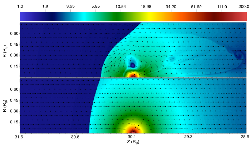
Figure 4.— Density color maps in logarithmic scale, and velocity field at $t=1.5R_{B}/c_{\infty}$ (upper panel) and $t=15R_{B}/c_{\infty}$ (lower panel) for a gravitational body with $\mathcal{A}=50$ and $\mathcal{M}=1.5$. The gas is adiabatic.

4. The nonlinear supersonic case: The values of $\tilde{\lambda}$

The complex and multidimensional dynamics of the flow in core potentials has been studied in the adiabatic nonlinear case by KK09 and, more recently, by Naiman et al. (2011), including also the isothermal cases. The latter authors, however, were interested in the accumulation of mass around the center of the potential and did not report on the drag force. In order to have a reliable estimate of the drag force, we carried out (adiabatic) numerical simulations varying $\mathcal{A}$ between $8$ and $50$, for various Mach numbers. In our simulations, we fixed $M$, $\rho_{\infty}$ and $c_{\infty}$ and only ${\mathcal{M}}$ and ${\mathcal{A}}$ vary from one simulation to another. For $G=M=c_{\infty}=1$, the time unit is $R_{B}/c_{\infty}$ and so we define the dimensionless time as $\tilde{t}=(c_{\infty}/R_{B})t$. In these units, given ${\mathcal{A}}$ and $\mathcal{M}$, it holds that $R_{s}=1/{\mathcal{A}}$ and $V=\mathcal{M}$.

We found that the dynamics of our simulated flow is consistent with those performed in KK09 and Naiman et al. (2011). For subsonic perturbers, we confirmed the result by KK09 that the nonlinear drag force reaches an asymptotic value that is similar to the drag in the linear case, as given in Eq. (2), regardless the value of $\mathcal{A}$. Therefore, we will not discuss the subsonic case any further; the reader interested in the subsonic case is referred to KK09.

Figure 5.— Dimensionless drag force using three analytical formulae (Ostriker’s formula [Eq. 3] with $r_{\rm min}=2.25R_{s}$ [dashed line]; Eq. 11 with $\tilde{\lambda}=1.25$ [implying $r_{\rm min}=1.25R_{B}$, dotted line]; and KK09 formula [Eq. 13, dot-dashed line]), as compared with the measured values from the simulation, for a body with $\mathcal{M}=1.5$ and $\mathcal{A}=20$. The left-hand panel shows them as a function of time, whereas the right-hand panel shows the ratio between the values obtained in the simulation $F_{\rm sim}$ and the values when the abovementioned analytical equations are used.

Figure 6.— Dimensionless drag force at $\tilde{t}=11.3$, as a function of $\mathcal{A}$ for a perturber with $\mathcal{M}=2.5$ (asterisks). The dashed line represents the drag force derived in the linear approximation (Equation 12 with $\lambda=2.25$).

For supersonic perturbers with ${\mathcal{A}}\gtrsim 1$, the linear analysis cannot capture the flow dynamics in regions with high spatial gradients; that is, on the surface of the Mach cone and at distances $r\lesssim R_{B}$ from the perturber. In Figure 4, we plot the density color maps and the velocity field of the flow around a perturber with $\mathcal{M}=1.5$ and $\mathcal{A}=50$. As already described by KK09, a bow shock thermalizes the upstream flow, leading to the formation of an envelope of highly subsonic gas in quasi-hydrostatic equilibrium. In fact, since the flow at infinity is laminar, shocks may occur for those streamlines that are bent significantly. Streamlines with impact parameters $b$ obeying the condition

$$\frac{2GM}{\sqrt{b^{2}+R_{s}^{2}}}<c_{\infty}^{2}+V_{0}^{2},$$ (9)

will bend significantly and terminate in a shock (e.g., Krumholz et al. 2005). In terms of $R_{A}$, this condition for strong bending can be written as

$$b<\left(R_{A}^{2}-R_{s}^{2}\right)^{1/2}.$$ (10)

In a case where ${\mathcal{A}}\gg 1$, then $R_{s}\ll R_{A}$, condition that reduces to $b<R_{A}$. The incoming supersonic flow moving close to the axis of symmetry collides with streamlines that have larger impact parameters but have been bent by the gravitational potential, leading to the formation of a detached bow shock. We find that for $\mathcal{M}=1.5$ and $\mathcal{A}=50$, the stand-off distance of the bow shock to the perturber along the symmetry axis ($R=0$), denoted by $\delta$, is $\sim 0.56R_{B}=0.9R_{A}$, which is in good agreement with the value reported in KK09 (see their Figure 12). Since the contribution to the drag force of material within a sphere of radius $\sim\delta$ is very small, because of the front-back symmetry, we expect $r_{\rm min}\gtrsim R_{A}$, which implies $\tilde{\lambda}\gtrsim 2/(1+\mathcal{M}^{2})$ in the deep nonlinear regime (remind that $r_{\rm min}=\tilde{\lambda}R_{B}$).

In a situation where $R_{A}\gg 2.25R_{s}$ (which also implies that $R_{B}\gg 2.25R_{s}$), one expects that the relevant minimum radius $r_{\rm min}$ for the gravitational interaction will be solely determined by $R_{B}$ and $\mathcal{M}$, because $R_{s}$ becomes irrelevant as far as the drag force concerns. Under these circumstances, the drag force, as a function of $\tilde{t}$, is expected to be independent of $\mathcal{A}$:

$$\frac{F_{DF}}{F_{0}}=\frac{1}{\mathcal{M}^{2}}\left[\frac{1}{2}\ln\left(1-\mathcal{M}^{-2}\right)+\ln\left(\frac{\mathcal{M}\tilde{t}}{\tilde{\lambda}}\right)\right].$$ (11)

The parameter $\tilde{\lambda}$ that connects $r_{\rm min}$ with $R_{B}$ may be a complex function of the Mach number $\mathcal{M}$, but it should also depend on the equation of state (i.e. on $\gamma$ for polytropic gas). The condition $R_{A}\gg 2.25R_{s}$ can be written in terms of a critical value ${\mathcal{A}}_{\rm cr}$, as $\mathcal{A}\gg\mathcal{A}_{\rm cr}$, with $\mathcal{A}_{\rm cr}=\mathcal{M}^{2}+1$. For a typical value of $\mathcal{M}$, say $\mathcal{M}=2$, $\mathcal{A}_{\rm cr}=5$.

Figure 7.— Drag force as a function of time for $\mathcal{A}=20$ (solid lines) and $\mathcal{A}=50$ (dashed lines). The correponding Mach number is quoted at the corner of each panel. The dotted curves give the drag force using Equation (11) with $\tilde{\lambda}=0.33$ (top panel), $\tilde{\lambda}=1.20$ (middle panel) and $\tilde{\lambda}=2.54$ (lower panel).

Figure 5 shows the drag force as a function of $\tilde{t}$ for a body moving at $\mathcal{M}=1.5$ and $\mathcal{A}=20$ (thus, $\mathcal{A}>\mathcal{A}_{\rm cr}=3.25$). We see that, at $\tilde{t}>3$, Eq. (11) with $\tilde{\lambda}=1.25$ (implying that $r_{\rm min}=1.25R_{B}$) reproduces the mean amplitude (not the fluctuations) and temporal evolution of the drag force fairly well. For comparison, we also plot $F_{\rm lin}$, that is, the drag force using Ostriker’s formula (Eqs. 1 and 3) with $r_{\rm min}=2.25R_{s}$. If the time is measured in units of $R_{B}/c_{\infty}$, $F_{\rm lin}$ is given by

$$\frac{F_{\rm lin}}{F_{0}}=\frac{1}{\mathcal{M}^{2}}\left[\frac{1}{2}\ln(1-\mathcal{M}^{-2})+\ln\left(\frac{{\mathcal{A}}\mathcal{M}\tilde{t}}{\lambda}\right)\right],$$ (12)

with $\lambda\simeq 2.25$ (see Section 3). As expected, a value of $r_{\rm min}=2.25R_{s}$ overestimates the drag force at any time.

KK09 suggested an empirical relation between $F_{DF}$ and $F_{\rm lin}$ through the parameter $\eta\equiv\mathcal{A}/(\mathcal{M}^{2}-1)$. They found that

$$F_{DF}=(\eta/2)^{-0.45}F_{\rm lin},$$ (13)

for $2\leq\eta\leq 100$. Figure 5 shows that the ratio $F_{DF}/F_{\rm lin}$ is not constant with time; its value is always larger than $(\eta/2)^{-0.45}=0.39$, implying that KK09 prescription underestimates the drag force. The ratio $F_{DF}/F_{\rm lin}$ is not constant with time but approaches asymptotically to $1$ when $\tilde{t}\rightarrow\infty$, i.e. when the contribution of the inner part of the wake to the gravitational drag becomes small as compared to the contribution of the far-field wake, which increases logarithmically with time. In fact, at times $t\gg R_{B}/V_{0}$, the nonlinear part of the wake has reached a quasistationary regime; $F_{DF}$ increases with time due to the new material that is incorporated into the wake in the far field, which can be described in linear theory. This implies that $dF_{DF}/dt=dF_{\rm lin}/dt$. Therefore, at large enough times, what is constant with time is the difference $F_{\rm lin}-F_{DF}=F_{0}\ln(\tilde{\lambda}R_{B}/[\lambda R_{s}])=\ln(\tilde{\lambda}\mathcal{A}/\lambda)$. The formula $F_{DF}=(\eta/2)^{-0.45}F_{\rm lin}$ may induce a significant fractional error at large Coulomb logarithms.

Figure 6 shows the drag force at $\tilde{t}=11.3$ for a perturber with $\mathcal{M}=2.5$ and differing ${\mathcal{A}}$. Note that $\mathcal{A}_{\rm cr}=7$ in this case. We see that the drag force when ${\mathcal{A}}<8$ increases linearly with $\ln{\mathcal{A}}$, as predicted in linear theory (see Eq. 12). For ${\mathcal{A}}>8$, the drag force is essentially constant with ${\mathcal{A}}$. The transition between the linear regime and the plateau, where the force becomes almost constant, is abrupt.

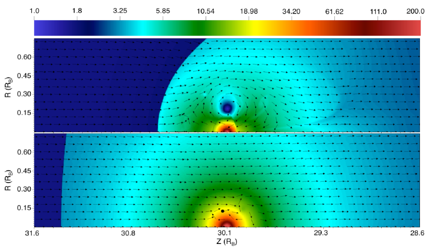
Figure 8.— Density color maps in logarithmic scale and velocity field at $t=1.5R_{B}/c_{\infty}$ (upper panel) and $t=15R_{B}/c_{\infty}$ (lower panel) for a gravitational body with $\mathcal{A}=50$ and $\mathcal{M}=1.15$. The gas is adiabatic.

Figure 7 shows the drag force, as a function of time, for $\mathcal{M}=2.5,1.5$, and $1.15$, with $\mathcal{A}=20$, and $50$. The drag force displays some oscillations with time, but the amplitudes of the drag force for $\mathcal{A}=20$ and $\mathcal{A}=50$ are similar. At Mach numbers $1.5$ and $2.5$, Equation (11) predicts the amplitude of the drag force correctly for $\tilde{\lambda}=0.33$ and $\tilde{\lambda}=1.2$, respectively. This clearly shows that $\tilde{\lambda}$ depends strongly on $\mathcal{M}$. At Mach number $1.15$, a $\tilde{\lambda}$-value of $2.54$ is required to fit the amplitude of the drag force at $\tilde{t}=12$–$14$, but it fails to reproduce the strength of the drag force at shorter times. In fact, as the Mach number approaches to $1$, an increasingly longer time is required until the drag force increases logarithmically in time. Thus, Equation (11) is not a good approximation at early times in those cases. The reason is that perturbers moving at speed near Mach $1$, can sustain a large envelope of gas, and the time required for the perturber to establish such a quasi-stationary density envelope increases when $\mathcal{M}\rightarrow 1$. This is illustrated in Figure 8. We see the temporal evolution of the bow shock and the formation of the envelope for a perturber moving at $\mathcal{M}=1.15$, and with $\mathcal{A}=50$. For this transonic Mach number, the distance of the bow shock at $\tilde{t}=15$ is a factor of $2$ larger than for $\mathcal{M}=1.5$. This explains why the minimum radius is larger at $\mathcal{M}=1.15$ than it is at $\mathcal{M}=1.5$.

Figure 9.— Measured dimensionless drag force at $\tilde{t}=11.3$, as a function of $\mathcal{M}$, for $\mathcal{A}=20$ (asterisks) and $\mathcal{A}=50$ (diamonds). The lines shown are the predicted values using Equation (11) with $\tilde{\lambda}=3.3\mathcal{M}^{-2.5}$ (solid line), with $\tilde{\lambda}=2\mathcal{M}^{-2}$ (dotted line) and with $\tilde{\lambda}=2/(\mathcal{M}^{2}+1)$ (dashed line). The drag force using Equation (13) with $\mathcal{A}=50$ is also shown (dot-dashed line).

Figure 9 shows the drag force at $\tilde{t}=11.3$, as a function of Mach number. As reported in KK09, the Mach number corresponding to the maximum drag force shifts from unity to $\sim 1.5$ as the wake becomes highly nonlinear. A minimum radius with $\tilde{\lambda}=3.3\mathcal{M}^{-2.5}$ provides a good fit to the drag force for Mach numbers between $1.5$ and $3$. As already said, at Mach numbers close to $1$, the value of $\tilde{\lambda}$ cannot be established because, at those times, Eq. (11) does not provide a good description of the temporal behaviour of $F_{DF}$. It is important to note that at Mach numbers $\geq 2$, $\tilde{\lambda}=2/(\mathcal{M}^{2}+1)$ provides a good fit, but especially a power law $\tilde{\lambda}=2.0\mathcal{M}^{-2}$, implying that $r_{\rm min}=2GM/V_{0}^{2}$, gives a better fit.

It is interesting to consider the point-mass case as the limit when $R_{s}=0$. The structure of the wake past a body with a nonzero $R_{s}$ is different to a case where $R_{s}=0$. In the first case, there is conservation of mass in the whole computational domain, whereas in the second case one must implement an inner boundary condition where “accreted” gas particles are sinked. Cantó et al. (2011) studied the point-mass case in the hypersonic case and found $r_{\rm min}\simeq 0.8GM/V_{0}^{2}$. Therefore, although the flow past a point-mass accretor is different to the flow past a non-accretor, the minimum impact parameter in the drag force might be relatively similar.

5. Discussion and conclusions

The interaction between a gravitational perturber and the ambient medium is a classical problem in astrophysics (e.g., Bondi & Hoyle 1944). Star clusters moving in cold interstellar gas, globular clusters in gaseous halos, galaxies moving through the intergalactic or intracluster medium, can be described as core potentials. In these systems, it is usually assumed that their individual members are accreting at so low enough rates that the mass is conserved (i.e. gas removal due to accretion can be neglected, see e.g., Naiman et al. 2011). In this paper, we have studied the gravitational drag force (dynamical friction) that their own induced wake produces on this kind of objects. To do so, we have modelled them as Plummer perturbers and the gas is assumed adiabatic. We have studied both the linear and nonlinear regimes.

In the supersonic linear regime, the maximum of the mass density in the wake created by a core (non-diverging) potential is not situated at the minimum of the gravitational potential but it is placed behind it. In the linear regime, the minimum radius $r_{\rm min}$ cannot be much larger than a few softening radii because beyond those distances from the perturber, the wake density is almost undistinguishable from the wake created by a point mass. In particular, for the Plummer sphere with core radius $R_{s}$, we confirm our previous result that the minimum radius for the drag force is $\sim 2.25R_{s}$. Thus, $r_{\rm min}$ is fairly independent of the Mach number. We must emphasize that in the linear regime, the dependence on the particular radiative cooling and heating of the gas is through the sound speed $c_{\infty}$.

If we keep $R_{B}$ fixed and reduce $R_{s}$, we have models with higher $\mathcal{A}$ and, hence, the gas dynamics around the body becomes nonlinear. When $R_{B}\gg R_{s}$ (i.e. $\mathcal{A}\gg 1$), the radius $R_{s}$ becomes irrelevant as far as the drag force is concerned. Thus, the minimum radius $r_{\rm min}$ must be related with the Bondi scale and/or the “accretion” radius. Using axisymmetrical simulations, we found that the drag force can be described well by using Ostriker (1999) formula with $r_{\rm min}=3.3\mathcal{M}^{-2.5}R_{B}$ for perturbers with $\mathcal{M}\geq 1.5$ and $\mathcal{A}>\mathcal{A}_{\rm cr}\equiv\mathcal{M}^{2}+1$. However, at $\mathcal{M}>2$, the drag force can be equally explained using $r_{\rm min}=2\mathcal{M}^{-2}R_{B}$ or $r_{\rm min}=R_{A}$. The latter possibilities imply that $r_{\rm min}=2GM/V_{0}^{2}$ at the hypersonic limit, which resembles the scaling found for a point-mass (accreting) perturber by Cantó et al. (2011).

At large enough times, the wake can be decomposed into the nonlinear part, which has reached a quasi-stationary state and a growing far-field wake. Our working formula for the drag force naturally includes the fact that at times $\gg R_{B}/c_{\infty}$, the material that is being incorporated into the wake has large impact parameters and thus can be described using the linear theory, implying that $dF_{DF}/dt=dF_{\rm lin}/dt$. On the contrary, the formula proposed by KK09, $F_{DF}=(\eta/2)^{-0.45}F_{\rm lin}$, does not match this condition, meaning that this relationship between $F_{DF}$ and $F_{\rm lin}$ should break down at a certain $t$. We tested KK09 formula and found that it underestimates the drag force, especially at large times (long wakes).

Applied to a perturber in orbit, KK09 argue that since $F_{DF}\propto M^{1.55}$, then the orbital decay timescale of a cored perturber declines as $\tau_{\rm dec}\propto M^{-0.55}$ (e.g., Binney & Tremaine 1987). Our formula has the classical dependence $F_{DF}\propto M^{2}\ln\Lambda$, where the dependence of $\ln\Lambda$ on $M$ is very weak. Thus, perturbers with an initial orbital radii much larger than $R_{B}$ decay in a characteristic timescale $\propto M^{-1}$.

References

- Binney & Tremaine (1987) Binney, J., & Tremaine, S. 1987, Galactic Dyanamics, Princeton Series in Astrophysics, Princeton University Press
- Bondi & Hoyle (1944) Bondi, H., & Hoyle, F. 1944, MNRAS, 104, 273
- Cantó et al. (2011) Cantó, J., Raga, A. C., Esquivel, A., Sánchez-Salcedo, F. J. 2011, MNRAS, 418, 1238
- Cantó et al. (2012) Cantó, J., Esquivel, A., Sánchez-Salcedo, F. J., & Raga, A. C. 2012, ApJ, 762, 21
- Dokuchaev (1964) Dokuchaev, V. P. 1964, Soviet Astron., 8, 23
- Fryxell et al. (2000) Fryxell, B., et al. 2000, ApJS, 131, 273
- Furlanetto & Loeb (2002) Furlanetto, S. R., & Loeb, A. 2002, ApJ, 565, 854
- Hunt (1971) Hunt, R. 1971, MNRAS, 154, 141
- Hunt (1979) Hunt, R. 1979, MNRAS, 188, 83
- Just & Kegel (1990) Just, A., & Kegel, W. H. 1990, A&A, 232, 447
- Kim & Kim (2009) Kim, H., & Kim, W.-T. 2009, ApJ, 703, 1278
- Krumholz, McKee & Klein (2005) Krumholz, M. R., McKee, C. F., & Klein, R. I. 2005, ApJ, 618, 757
- Lee & Stahler (2011) Lee, A. T., & Stahler, S. W. 2011, MNRAS, 416, 3177
- Naiman et al. (2011) Naiman, J. P., Ramírez-Ruiz, E., & Lin, D. N. C. 2011, ApJ, 735, 25
- Ostriker (1999) Ostriker, E. C. 1999, ApJ, 513, 252
- Rein (2012) Rein, H. 2012, MNRAS, 422, 3611
- Ruderman & Spiegel (1971) Ruderman, M. A., & Spiegel, E. A. 1971, ApJ, 165, 1
- Ruffert (1994) Ruffert, M. 1994, A&AS, 106, 505
- Ruffert (1996) Ruffert, M. 1996, A&A, 311, 817
- Sánchez-Salcedo (2009) Sánchez-Salcedo, F. J., 2009, MNRAS, 392, 1573
- Sánchez-Salcedo (2012) Sánchez-Salcedo, F. J., 2012, ApJ, 745, 135