Super-intense highly anisotropic optical transitions in anisotropic quantum dots

Abstract

Coulomb interaction among electrons is found to have profound effects on the electronic properties of anisotropic quantum dots in a perpendicular external magnetic field, and in the presence of the Rashba spin-orbit interaction. This is more evident in optical transitions, which we find in this system to be highly anisotropic and super-intense, in particular, for large values of the anisotropy parameter.

For more than two decades, theoretical studies of quantum dots (QDs) in an external magnetic field maksym , have largely focused on the properties of dots with circular symmetry qdbook ; heitmann . Extensive investigations of transport and optical spectroscopy of these semiconductor nanostructures (the artificial atoms) have revealed several important atomic-like properties qdbook ; heitmann . In contrast, not enough is known about the electronic properties of anisotropic quantum dots madhav ; elliptic_expt . Another important direction of the QD research that is gaining popularity in recent years has been the role of Rashba spin-orbit interaction (SOI) rashba ; halperin ; note_Dr in quantum dots. The importance of this interaction in semiconductor spintronics has been well documented in the literature spintro ; nitta ; SOI_dot . Detailed theoretical studies of the influence of Rashba SOI on the electronic properties of QDs with isotropic confinement have already been reported earlier rashba_tc , where the SO coupling was found to manifest itself mainly in multiple level crossings and level repulsions in the energy spectra. These were attributed to an interplay between the Zeeman effect and the SOI present in the system Hamiltonian. Those effects, in particular the level repulsions, were weak and as a result, would require extraordinary efforts to detect the strength of SO coupling tunneling in those systems. On the other hand, by introducing anisotropy in a QD, we have previously shown that a major enhancement of the Rashba SO coupling effects can be achieved in the Fock-Darwin spectra siranush . Although various approximate schemes exist to study the effects of anisotropy on the far-infrared absorption vidar , the role of SO coupling on the far-infrared response serra , or other physical properties of elliptical dots others , an accurate and coherent theoretical treatment of all these issues, in particular, the role of Coulomb interaction, in conjunction with all these properties, is seriously lacking. Here we demonstrate that in the presence of the Coulomb interaction among the electrons, and combined with the Rashba SOI, the eccentricity of the QD is responsible for major modification of the electron energy spectra, which clearly manifests itself in super-intense, and highly anisotropic optical transitions that is vastly different from those that are commonly observed in an isotropic QD.

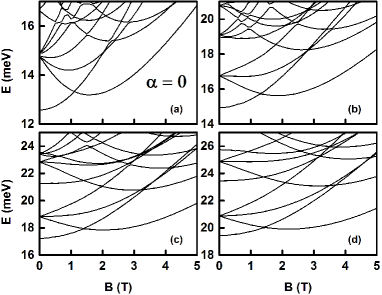
Figure 1: Magnetic field dependence of the low-lying two-electron energy levels of an elliptical dot without the Rashba SOI $(\alpha=0)$. The results are for $\omega_{x}=4$ meV and (a) $\omega_{y}=4.1$ meV, (b) $\omega_{y}=6$ meV, (c) $\omega_{y}=8$ meV, and (d) $\omega_{y}=10$ meV.

Until now, interacting electrons in elliptical QDs have been studied by means of perturbative approaches elliptic_int . In what follows, we present a non-perturbative, exact diagonalization scheme to treat interacting electrons in anisotropic quantum dots. Our complete single-particle Hamiltonian of an electron moving in the $xy$-plane and subjected to an external perpendicular magnetic field with the vector potential $\mathbf{A}=\frac{1}{2}B(-y,x)$ is

$${\cal H} = \frac{1}{2m_{e}}\left(\mathbf{p}-\frac{e}{c}\mathbf{A}\right)^{2}+\tfrac{1}{2}m_{e}\left(\omega_{x}^{2}x^{2}+\omega_{y}^{2}y^{2}\right)$$

$$+\frac{\alpha}{\hbar}\left[\bm{\sigma}\times\left(\mathbf{p}-\frac{e}{c}\mathbf{A}\right)\right]_{z}+\tfrac{1}{2}g\mu_{B}B\sigma_{z}.$$

The first two terms on the right hand side describe a two-dimensional harmonic oscillator confined by an elliptic potential madhav . The next term takes care of the SOI while the last one is for the Zeeman coupling. In order to treat the Coulomb interaction we rearrange the terms in the Hamiltonian into three parts

$${\cal H}_{\Lambda} = \frac{1}{2m_{e}}\left(p_{x}^{2}+p_{y}^{2}+\Omega_{x}^{2}x^{2}+\Omega_{y}^{2}y^{2}\right);\ \ {\cal H}_{Z}=\tfrac{1}{2}g\mu_{B}B\sigma_{z}$$

$${\cal H}_{R} = \tfrac{1}{2}\omega_{c}(yp_{x}-xp_{y})+\frac{\alpha}{\hbar}\left[\sigma_{x}\left(p_{y}-\frac{eB_{\perp}}{2c}\,x\right)\right.$$

$$\left.-\sigma_{y}\left(p_{x}+\frac{eB_{\perp}}{2c}\,y\right)\right],$$

where ${\cal H}_{\Lambda}$ describes a two-dimensional spinless harmonic oscillator, the Zeeman coupling ${\cal H}_{Z}$ introduces the spin and ${\cal H}_{R}$ deforms the simple Cartesian phase space of the operators ${\cal H}_{\Lambda}$ and ${\cal H}_{Z}$. We have also introduced the cylotron frequency $\omega_{c}=eB/{m_{e}c}$ and the oscillator frequences $\Omega_{x,y}^{2}=m_{e}^{2}\left(\omega_{x,y}^{2}+\tfrac{1}{4}\omega_{c}^{2}\right).$ The eigenstates $|\lambda\rangle$ of the oscillator Hamiltonian ${\cal H}_{\Lambda}$ are just direct products $|n^{\lambda}_{x}\rangle|n^{\lambda}_{y}\rangle$ of the two harmonic oscillator states represented by the quantum numbers $n^{\lambda}_{x,y}$. Inclusion of the Zeeman term is also straightforward: we multiply the states $|\lambda\rangle$ with the eigenstates $|s_{z}\rangle$ of the Pauli spin matrix $\sigma_{z}$ yielding the states $|\xi\rangle=|\lambda^{\xi}\rangle|s^{\xi}_{z}\rangle.$ Finally, the effects of the operator ${\cal H}_{R}$ are incorporated by diagonalizing it in the base spanned by the eigenstates $|\xi\rangle$ of the combination ${\cal H}_{\Lambda}+{\cal H}_{Z}$. Thus the eigenstates $|\gamma\rangle$ of the total single electron Hamiltonian ${\cal H}$ are experessed as superpositions of the states $|\xi\rangle$.

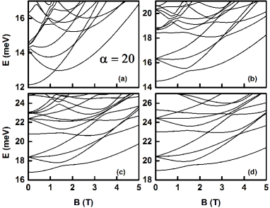
Figure 2: Same as in Fig. 1, but for $\alpha=20$ meV.nm.

To handle the mutual interactions between electrons, we work in the occupation number representation based on the eigenstates of the Hamiltonian ${\cal H}$. Then the main task is to evaluate the two-body matrix elements

$$\langle\gamma_{1}\gamma_{2}|V|\gamma_{3}\gamma_{4}\rangle = \int\mbox{d}\mathbf{x}_{1}\,\mbox{d}\mathbf{x}_{2}\,\Phi_{\gamma_{1}}^{\ast}(\mathbf{x}_{1})\Phi_{\gamma_{2}}^{\ast}(\mathbf{x}_{2})$$

$$\times V(|\mathbf{x}_{1}-\mathbf{x}_{2}|)\Phi_{\gamma_{3}}(\mathbf{x}_{2})\Phi_{\gamma_{4}}(\mathbf{x}_{1}),$$

where the wave functions $\Phi_{\gamma}(\mathbf{x})$ correspond to the eigenstates $|\gamma\rangle$ of ${\cal H}$ and the integrals over the variables $\mathbf{x}$ include also summation over the spin degrees of freedom. The expansion of the functions $\Phi_{\gamma}$ in terms of the wave functions corresponding to the eigenstates $|\xi\rangle$ of ${\cal H}_{\Lambda}+{\cal H}_{Z}$ leads to evaluations of two-body matrix elements between the states $|\xi\rangle$. Since the electrons act via the Coulomb potential $V(|\mathbf{x}|)=V_{C}(r)=e^{2}/\epsilon r$, where $\epsilon$ is the background dielectric constant, the summations over spin degrees of freedom yield only Kronecker delta’s of the $s_{z}$ quantum numbers and we are left with the matrix elements

$$\langle\lambda_{1}\lambda_{2}|V|\lambda_{3}\lambda_{4}\rangle = \int\mbox{d}\mathbf{r}_{1}\,\mbox{d}\mathbf{r}_{2}\,\psi_{\lambda_{1}}^{\ast}(\mathbf{r}_{1})\psi_{\lambda_{2}}^{\ast}(\mathbf{r}_{2})$$

$$\times V(|\mathbf{r}_{1}-\mathbf{r}_{2}|)\psi_{\lambda_{3}}(\mathbf{r}_{2})\psi_{\lambda_{4}}(\mathbf{r}_{1})$$

between pairs of the single-particle oscillator wave functions. In isotropic parabolic dots with mutual Coulomb interactions we could use the explicit algebraic formula rashba_tc , but in elliptical confinements we have to resort to numerical computations. Perhaps the most cost-effective way is to do the evaluation via the Fourier transforms

$$\tilde{\Psi}_{\mu\nu}(\mathbf{k}) = \int\mbox{d}\mathbf{r}\,\mathrm{e}^{\mathrm{i}\mathbf{k}\cdot\mathbf{r}}\psi_{\mu}^{\ast}(\mathbf{r})\psi_{\nu}(\mathbf{r})$$

$$\tilde{V}(\mathbf{k}) = \int\mbox{d}\mathbf{r}\,\mathrm{e}^{\mathrm{i}\mathbf{k}\cdot\mathbf{r}}V(\mathbf{r})$$

of the products of the wave functions and the interaction. A straightforward algebra yields the expression

$$\langle\lambda_{1}\lambda_{2}|V|\lambda_{3}\lambda_{4}\rangle=\frac{1}{(2\pi)^{2}}\int\mbox{d}\mathbf{k}\,\tilde{\Psi}_{\lambda_{4}\lambda_{1}}^{\ast}(\mathbf{k})\tilde{\Psi}_{\lambda_{2}\lambda_{3}}(\mathbf{k})\tilde{V}(\mathbf{k}).$$

Numerical computation of this final two-fold integral is a relatively fast operation.

Figure 3: Same as in Fig. 1, but for $\alpha=40$ meV.nm.

Since for the Coulomb interactions we know the Fourier transform to be $\tilde{V}_{C}(\mathbf{k})=2\pi e^{2}/\epsilon\,k,$ we are left with the evaluation of the Fourier transforms $\tilde{\Psi}_{\mu\nu}(\mathbf{k})$. We have experimented with two practically equally efficient methods: the first one is fully generic and applicable to any system while the second one is restricted to elliptical confinements. The generic method is based on the observation that the Fourier transform $\tilde{\Psi}_{\mu\nu}(\mathbf{k})$ can in fact be written as the matrix element of the exponential of the position operator $\mathbf{r}_{\mathrm{op}}$, $\tilde{\Psi}_{\mu\nu}(\mathbf{k})=\left\langle\mu\left|\mathrm{e}^{\mathrm{i}\mathbf{k}\cdot\mathbf{r}_{\mathrm{op}}}\right|\nu\right\rangle$. Since the components $x_{\mathrm{op}}$ and $y_{\mathrm{op}}$ of the position operator commute we actually need the matrix elements of the exponential operators $\exp\left(\mathrm{i}x_{\mathrm{op}}\right)$ and $\exp\left(\mathrm{i}y_{\mathrm{op}}\right)$. These in turn are easily evaluated by diagonalizing the matrix $X$ with matrix elements $X_{\mu\nu}=\left\langle\mu\left|x_{\mathrm{op}}\right|\nu\right\rangle$ and applying the inverse unitary transformation taking $X$ to the diagonal form to the exponentiated diagonal, together with the similar procedure for the operator $y_{\mathrm{op}}$.

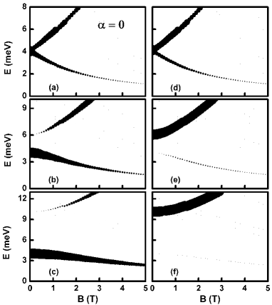
Figure 4: Optical absorption (dipole allowed) specta of elliptical QDs with $\alpha=0$ meV.nm for various choice of anisotropy parameters: (a) $\omega_{x}=4$ meV, $\omega_{y}=4.1$, (b) $\omega_{x}=4$ meV, $\omega_{y}=6$ meV, and (c) $\omega_{x}=4$, $\omega_{y}=10$. The polarization of the incident radiation is along the $x$-axis. The parameters for (d)-(f) are the same, except that the incident radiation is polarized along the $y$-axis. The areas of the filled circles are proportional to the calculated absorption cross-section.

In the second approach we take advantage of the fact that the single-particle wave functions are products of two Hermite functions, one with the $x$-coordinate and the other with the $y$-coordinate as the argument. This implies that the product $\psi_{\mu}^{\ast}(\mathbf{r})\psi_{\nu}(\mathbf{r})$ to be transformed factorizes to a product of two functions depending on $x$ and $y$, respectively. In fact we can do the resulting one-dimensional transforms yielding

$$\tilde{\Psi}_{\mu\nu}(\mathbf{k})=\tilde{\cal G}^{x}_{n^{\mu}_{x},n^{\nu}_{x}}(k_{x})\tilde{\cal G}^{y}_{n^{\mu}_{y},n^{\nu}_{y}}(k_{y}),$$

where the functions $\tilde{\cal G}^{x,y}_{i,j}(k)$ are given by

$$\tilde{\cal G}^{x,y}_{ij}(k) = (-1)^{m}\sqrt{\frac{n!}{(n+\xi)!}}\,(\beta_{x,y}k)^{\xi}\,\mathrm{e}^{-\frac{1}{2}(\beta_{x,y}k)^{2}}$$

$$\times L_{n}^{\xi}\left((\beta_{x,y}k)^{2}\right)(\delta_{p,0}+\mathrm{i}\delta_{p,1}).$$

In the above formulas the symbols $n^{\mu}_{x,y}$ and $n^{\nu}_{x,y}$ stand for the $x$ and $y$ oscillator quantum numbers of the states labelled by $\mu$ and $\nu$. We have also introduced the shorthand notations $\beta_{x,y}=\sqrt{\frac{\hbar}{2m_{e}\omega_{x,y}}},\,n=\min(i,j),\,\xi=|i-j|,\,p=\xi\,\mbox{mod\,}2.$ Although both approaches introduced here have their merits, it should be noted that the first method is somewhat more general and applicable to any systems, while the second method works only for the harmonic oscillator basis. The second method is however computationally slightly faster than the first.

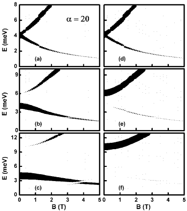
Figure 5: Same as in Fig. 4, but for $\alpha=20$ meV.nm.

In our numerical studies that follow, we have used the parameters corresponding to InAs QD siranush , where strong SOI was reported experimentally SOI_dot . The results for the energy spectra are displayed in Figs. (1 - 3) for various values of the SO coupling strength $\alpha$ and the anisotropy. In the absence of the external magnetic field and the SOI, neither the total spin $S$ nor its $z$-component $S_{z}$ appear in the full Hamiltonian (with Coulomb interactions). We therefore expect the two-electron systems to consist of $S=0$ spin singlets and $S=1$ spin triplets. The energy spectra of Fig. 1 indeed confirm that to be the case: the dispersions form bunches of one and three lines, the latter of which diverges due to the Zeeman splitting when the magnetic field increases. Perhaps the most noticeable feature shown in Fig. 1 is the singlet-triplet transition of the ground state for magnetic fields slightly above 1 Tesla. The origin of this crossing of the dispersion lines can be traced to the crossing of the second and third lowest energy levels of the single-electron systems siranush .

Just as for the circular QD, the spin singlet-triplet transition (at B$\simeq 1.5$ Tesla in Fig. 1) is the only transition in the ground state. The critical field where the transition takes place is somewhat dependent on the method of calculation and the choice of material parameters elliptic_int . The main role of the Coulomb interaction is the upward shift of the spectral lines and lifting of the accidental degeneracies. Surprisingly, the interaction also practically freezes the movement of the singlet-triplet transition point to higher fields when the eccentricity increases. In the absence of the electron-electron interaction the transition point shifts about two Teslas whereas in the presence of the interactions the shift is only few tenths of a Tesla with the same eccentricities.

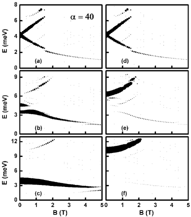
Figure 6: Same as in Fig. 5, but for $\alpha=40$ meV.nm.

When the SOI is turned on (Fig. 2 and Fig. 3) most of the characteristic features of Fig. 1 survive. However, since the SOI can mix spin-up and spin-down single-particle states, neither $S$ nor $S_{z}$ are any more good quantum numbers. This is clearly evident in the singlet-triplet transition which transforms to anticrossing in the presence of the SOI. Several similar kind of crossing-anticrossing conversions can also be seen higher in the spectra.

In Figs. 4–6 we show the the absorption cross sections for the dipole allowed transtions from the ground states corresponding to the energy spectra of Figs. 1–3, (a,b,d). We explore the cases where the incident radiation is polarized along the $x$ and $y$-direction. Since dipole absorptions involve only one electron we are effectively probing the single-particle properties of the dot, in particular, the oscillator strengths along the $x$ and $y$-directions. Consequently we expect the absorption sepectra to resemble approximately the spectra of the one-particle system. This indeed seems to be the case. Except for the case of almost isotropic QDs [(a) and (c)], the optical transitions are clearly highly anisotropic. For example, because the $y$-polarization probes for oscillations along the $y$-direction the related transitions go mostly to the upper mode, i.e., the favored transition energies are 4, 6 and 10 meV in Figs. (d)-(f). The resulting transitions are therefore super-intense, unlike in isotropic QDs. There are also weak-intensity transitions to the lower mode. This is due to the magnetic field and the SOI, both of which distort the confinement ellipsoid. There are of course some notable deviations from the single-electron case. For example, because the Coulomb interaction couples several non-interacting states there can be many more allowed transitions from a given interacting state than from a non-interacting one resulting in different absorption intensities.

To summarize: we have reported here very comprehensive and accurate studies of anisotropic quantum dots with interacting electrons in the presence of the Rashba SOI. We have shown here that the Coulomb interaction in the presence of the spin-orbit coupling has a very strong effect, particularly in the presence of strong anisotropy. This is clearly seen in the optical absorption spectra which is super-intense and highly anisotropic. The spectra derived here are entirely different from the ones observed thus far in isotropic QDs. Our present work can be generalized, in a straightforward manner, to include more interacting electrons in the QD. The energy spectra and the optical transitions with more electrons will undoubtedly be very complex. However, the basic properties uncovered here will remain intact. Those studies will be the subject of our future publications.

The work was supported by the Canada Research Chairs Program of the Government of Canada.

References

- (1) Electronic address: Tapash.Chakraborty@umanitoba.ca
- (2) P.A. Maksym and T. Chakraborty, Phys. Rev. Lett. 65, 108 (1990)
- (3) T. Chakraborty, Quantum Dots (North-Holland, Amsterdam, 1999);
- (4) D. Heitmann (Ed.), Quantum Materials (Springer, Heidelberg, 2010).
- (5) A.V. Madhav and T. Chakraborty, Phys. Rev. B 49, 8163 (1994).
- (6) A. Singha, V. Pellegrini, S. Kalliakos, B. Karmakar, A. Pinczuk, L.N. Pfeiffer, and K.W. West, Appl. Phys. Lett. 94, 073114 (2009); M. Hochgräfe, Ch. Heyn, and D. Heitmann, Phys. Rev. B 63, 035303 (2000); D.G. Austing, S. Sasaki, S. Tarucha, S.M. Reimann, M. Koskinen, M. Manninen, Phys. Rev. B 60, 11514 (1999).
- (7) Y.A. Bychkov and E.I. Rashba, J. Phys. C 17, 6039 (1984).
- (8) H.-A. Engel, B.I. Halperin, and E.I. Rashba, Phys. Rev. Lett. 95, 166605 (2005).
- (9) In InAs quantum well structures, the Dresselhaus SOI is quite appreciable, but the Rashba contribution is still dominant, see, e.g., S. Giglberger, et al., Phys. Rev. B 75, 035327 (2007).
- (10) For recent comprehensive reviews, see, T. Dietl, D.D. Awschalom, M. Kaminska, and H. Ono, (Eds.) Spintronics (Elsevier, Amsterdam, 2008); I. Zutic, J. Fabian, and S. Das Sarma, Rev. Mod. Phys. 76, 323 (2004); J. Fabian, A. Matos-Abiague, C. Ertler, P. Stano, and I. Zutic, Acta Physica Slovaca 57, 565 (2007); M.W. Wu, J.H. Jiang, and M.Q. Weng, Phys. Rep. 493, 61 (2010).
- (11) J. Nitta, T. Akazaki, H. Takayanagi, and T. Enoki, Phys. Rev. Lett. 78, 1335 (1997); M. Studer, G. Salis, K. Ensslin, D.C. Driscoll, and A.C. Gossard, ibid. 103, 027201 (2009); D. Grundler, ibid. 84, 6074 (2000).
- (12) H. Sanada, T. Sogawa, H. Gotoh, K. Onomitshu, M. Kohda, J. Nitta, and P.V. Santos, Phys. Rev. Lett. 106, 216602 (2011); S. Takahashi, R.S. Deacon, K. Yoshida, A. Oiwa, K. Shibata, K. Hirakawa, Y. Tokura, and S. Tarucha, ibid. 104, 246801 (2010); Y. Igarashi, M. Jung, M. Yamamoto, A. Oiwa, T. Machida, K. Hirakawa, and S. Tarucha, Phys. Rev. B 76, 081303 (R) (2007).
- (13) T. Chakraborty and P. Pietiläinen, Phys. Rev. Lett. 95, 136603 (2005); P. Pietiläinen and T. Chakraborty, Phys. Rev. B 73, 155315 (2006); T. Chakraborty and P. Pietiläinen, ibid. 71, 113305 (2005); A. Manaselyan and T. Chakraborty, Europhys. Lett. 88, 17003 (2009); and the references therein.
- (14) H.-Y. Chen, V. Apalkov, and T. Chakraborty, Phys. Rev. B 75, 193303 (2007).
- (15) S. Avetisyan, P. Pietiläinen, and T. Chakraborty, Phys. Rev. B 85, 153301 (2012); Phys. Rev. B 86, 269901 (E) (2012).
- (16) I. Magnusdottir and V. Gudmundsson, Phys. Rev. B 60, 16591 (1999).
- (17) L. Serra, M. Valin-Rodriguez, and A. Puente, Surf. Sci. 532 - 535, 576 (2003).
- (18) G. Rezaei, Z. Mousazadeh, B. Vaseghi, Physica E 42, 1477 (2010); L. Serra, A. Puente, and E. Lipparini, Int. J. Quant. Chem. 91, 483 (2003); E. Lipparini, L. Serra, and A. Puente, Eur. Phys. J. B 27, 409 (2002); M. van den Broek, and F.M. Peeters, Physica E 11, 345 (2001); I. Magnusdottir and V. Gudmundsson, Phys. Rev. B 61, 10229 (2000).
- (19) P.A. Maksym, Physica B 249- 251, 233 (1998); Y.-H. Liu, F.-H. Yang, and S.L. Feng, J. Appl. Phys. 101, 063714 (2007).