Ray-based analysis of the interference striation pattern in an underwater acoustic waveguide

Abstract

In some underwater acoustic waveguides with specially selected sound speed profiles striations or fringes of the interference pattern are determined by a single parameter $\beta$ called the waveguide (or Chuprov) invariant. In the present paper it is shown that an analytical description of fringes may be possible in a waveguide with an arbitrary sound speed profile. A simple analytical expression is obtained for smooth lines formed by local maxima of the interference pattern. This result is valid at long enough ranges. It is derived proceeding from a known relation connecting the differences of ray travel times and the action variables of ray paths.

PACS numbers: 43.30.Cq, 43.30.Dr

1 Formulation of the problem

Consider a transient wave field excited by a point source in a range-independent waveguide with the sound speed profile $c(z)$, where $z$ is the vertical coordinate directed downward. It is assumed that the source emitting a wideband regular or noise signal $s(t)$ is set at depth $z_{s}$. Signals arriving at a fixed depth $z=z_{r}$ form function $u(r,t)\,$, where $r$ is the source-receiver range.

Below we consider two characteristics of the wave field at depth $z_{r}$. One of them is $\Phi\left(r,\omega\right)=\left|\tilde{u}(r,\omega)\right|^{2}$, where $\tilde{u}\left(r,\omega\right)=\left(2\pi\right)^{-1}\int d\omega~{}u(r,t)e^{i\omega t}$. It represents the interference pattern in the range-frequency plane $\left(r,\omega\right)$. Local maxima and minima of $\Phi\left(r,\omega\right)$ form smoth curves which we call the interference lines and denote $\omega\left(r\right)$. The interference pattern consists of fringes (or striations) localized in the vicinities of the interference lines [1, 2, 3, 4, 5, 6, 7].

Another characteristic of the wave field is represented by the autocorrelation function

$$K\left(r,\tau\right)=\int dt~{}u(r,t+\tau)u^{\ast}\left(r,t\right)=2\pi\int d\omega~{}\Phi\left(r,\omega\right)e^{-i\omega\tau}.$$ (1)

It determines the interference pattern in the range–time delay plane $\left(r,\tau\right)$. In this plane also there are fringes localized in the vicinities of the interference lines $\tau\left(r\right)$.

In some waveguides with specially selected profiles $c(z)$ – we will call them the Chuprov waveguides – the interference lines are determined by simple equations

$$\frac{r}{\tau}\frac{d\tau}{dr}=-\beta,\;\frac{r}{\omega}\frac{d\omega}{dr}=\beta,$$ (2)

where $\beta$ is the so-called waveguide (or Chuprov) invariant [1, 2, 3]. In a Chuprov waveguide $\beta$ is the same constant for all the interference lines. Then Eqs. (2) are readily solved to yield

$$\tau(r)=~{}Cr^{-\beta},\omega(r)=C_{1}r^{\beta},$$ (3)

where $C$ and $C_{1}$ are some constants. Our objective in the present work is to derive an analytical expression for the interference line in a waveguide with an arbitrary sound speed profile.

2 Equation for the interference line

For solving this problem we will use the ray representation of the wave field [2, 8]. In the geometrical optics approximation the signal at observation point $\left(r,z_{r}\right)$ is presented in the form

$$u(r,t)=\sum_{n}u_{n}\left(r,t-t_{n}\right),$$ (4)

where $t_{n}$ is the travel time of the $n$-th eigenray, $u_{n}\left(t\right)$ is the sound pulse coming through this eigenray. The eigenrays are numbered in such a way that the same subscript $n$ at different ranges $r$ is associated with eigenrays with the same identifier $\left(N,\mu,\nu\right)$, where $N$ is the number of ray lower turning points (number of cycles), $\mu=\pm 1$ and $\nu=\pm 1$ determine the signs of the ray grazing angles at the end points [3].

According to Eq. (4), the autocorrelation function of the received sound signal is

$$K(r,\tau)=\sum_{n,m}q_{nm}(r,\tau-\tau_{nm}),$$ (5)

where $q_{nm}\left(r,\tau\right)=\int dt~{}u_{n}(r,t+\tau)u_{m}^{\ast}\left(r,t\right)$, $\tau_{nm}=t_{n}-t_{m}$. At a fixed range $r$, each term $q_{nm}\left(r,\tau\right)$ represents a peak with maximum at $\tau=0$ and width $O\left(1/\Delta f\right)$, where $\Delta f$ is the bandwidth of the emitted signal $s(t)$.

It follows from Eqs. (1) and (5) that

$$\Phi\left(r,\omega\right)=\sum_{n,m}\tilde{q}_{nm}\left(r,\omega\right)e^{i\omega\tau_{nm}(r)},\;$$ (6)

where $\tilde{q}_{nm}\left(r,\omega\right)=\left(2\pi\right)^{-2}\int d\tau~{}q\left(\tau\right)e^{i\omega\tau_{nm}(r)}$. According to Eqs. (5) and (6), the interference patterns in both planes $\left(r,\tau\right)$ and $\left(r,\omega\right)$ to a significant extent are determined by functions $\tau_{nm}(r)$.

Let us divide all the eigenrays arriving at the observation point $\left(r,z_{r}\right)$ in groups of fours. Each group includes eigenrays whose idenifiers $\left(N,\mu,\nu\right)$ have the same value of $N$ and different pairs $(\mu,\nu)$ [3]. If the source and receiver are located at relatively small depths – this case will be considered in the rest of this paper – the travel times of eigenrays belonging to the same group of four are close. The spread of these travel times is small compared to the difference between travel times of eigenrays from different groups. In Eq. (5) each pair of groups of four is presented by 16 terms which may strongly overlap. Their superposition form a fringe in the plane $\left(r,\tau\right)$ located in the vicinity of the interference line $\tau\left(r\right)=\tau_{nm}\left(r\right)$, where $\tau_{nm}$ is the difference between travel times of two eigenrays taken from two different groups. The value of $\tau_{nm}$ weakly depends on the choice of particular eigenrays taken from groups forming the fringe.

An approximate analytical expression for the interference line $\tau(r)$ can be derived proceeding from the known relation connecting the difference in ray travel times and the action variables of the ray paths [3, 9, 10, 11, 12]. Assume that the sound speed profile $c\left(z\right)$ has a single minimum at depth $z=z_{a}$. Then the action variable of a ray path intersecting the horizon $z_{a}$ at a grazing angle $\chi$ is [12]

$$I=\frac{1}{\pi}\int_{z_{\min}}^{z_{\max}}dz~{}\sqrt{c_{0}^{2}/c^{2}\left(z\right)-\cos^{2}\chi},$$ (7)

where $c_{0}=c(z_{a})$, $z_{\min}$ and $z_{\max}$ are the upper and lower ray turning depths, respectively. The cycle length of the ray path,

$$D=2\cos\chi\left.\int_{z_{\min}}^{z_{\max}}dz\right/~{}\sqrt{c_{0}^{2}/c^{2}\left(z\right)-\cos^{2}\chi},$$ (8)

can be considered as a function of the action $I$. We denote this function $D(I)$.

Take two eigerays connecting the source and receiver located at the same depth. We assume that the eigenrays have exactly $N+\Delta N$ and $N$ cycles of oscillations. The travel times of these eigenrays denote $t_{N+\Delta N}$ and $t_{N}$, respectively. Similarly, their action variables denote $I_{N+\Delta N}$ and $I_{N}$. The latter are determined by the relations

$$D(I_{N+\Delta N})=r/(N+\Delta N),\;D(I_{N})=r/N.$$ (9)

On condition that

$$N\gg\Delta N,$$ (10)

$I_{N+\Delta N}$ and $I_{N}$ are close and the difference between the eigenray travel times is given by the approximate relation [12, 13]

$$\tau=t_{N+\Delta N}-t_{N}=2\pi I\Delta N/c_{0},$$ (11)

where $I=\left(I_{N+\Delta N}+I_{N}\right)/2$. This relation was derived by different authors [3, 9, 10, 11]. The relationship between the ray travel times and action variables is studied in detail in monograph [12]. The monograph provides a detailed dervation of Eq. (11) and its generalizations.

If the distance between the source and receiver changes by a small amount $\delta r$, then the actions $I_{N+\Delta N}$ and $I_{N}$ change by $\delta I_{N+\Delta N}$ $\delta I_{N}$, respectively. It follows from Eqs. (9) and (10) that the mean value of action variables $I$ changes by

$$\delta I=\frac{1}{2}\left(\delta I_{N+\Delta N}+\delta I_{N}\right)\simeq\frac{D\left(I\right)}{D^{\prime}\left(I\right)}\frac{\delta r}{r},$$ (12)

where $D^{\prime}(I)=dD(I)/dI$. The corresponding change in the difference of travel times $\tau$ denote $\delta\tau$. According to Eq. (11), $\delta\tau/\tau=\delta I/I$. Substiting Eq. (12) in this relation yields the desired equation for the interference line

$$\frac{r}{\tau}\frac{d\tau}{dr}=-\beta\left(I\right),$$ (13)

where

$$\beta\left(I\right)=-\frac{D\left(I\right)}{ID^{\prime}\left(I\right)}.$$ (14)

Equation (14) relating the Chuprov parameter $\beta$ with the action variable of the ray path was obtained earlier in Ref. [14].

In the Chuprov waveguide $D(I)$ is a power function. Then $\beta$ does not depend on $I$ and has the same value for all the interference lines. An example is given by a waveguide with the sound speed profile

$$c(z)=c_{0}\sqrt{1+\left|\frac{z-z_{a}}{a}\right|^{g}},$$ (15)

where $c_{0}$, $a$ and $g$ are constants. For relatively flat rays in such a waveguide $D(I)\sim I^{(2-g)/(2+g)}$ and we find $\beta=(g+2)/(g-2)$ [3]. If $g=1$ formula (15) determines a waveguide with the squared index of refraction represented by a linear function of $z$. Then $\beta=-3$ [1, 2, 3]. Another well-known result is obtained for $g=\infty$. In this case $c(z)=c_{0}$ and we arrive at the Pekeris waveguide where $\beta=1$ [1, 2, 3].

Consider a fringe in a waveguide with an arbitrary sound speed profile formed by a pair of groups of four with $N+\Delta N$ and $N$ cycles of oscillation. Using Eq. (11), replace $I$ on the right-hand side of Eq. (14) by $\tau c_{0}/(2\pi\Delta N)$. This yields an equation for $\tau$ which is readily solved. It turns out that the interference line $\tau(r)$ which takes value $\tau_{0}$ at range $r_{0}$ is determined by the relation

$$\frac{D\left(\frac{c_{0}\tau}{2\pi\Delta N}\right)}{D\left(\frac{c_{0}\tau_{0}}{2\pi\Delta N}\right)}=\frac{r}{r_{0}}.$$ (16)

According to this formula, the shape of the interference line, generally, depends on $\Delta N$. Our assumption that the source and receiver have the same depths is made only to simplify the derivation of (16). This result remain valid for $z_{r}\neq z_{s}$. It should be emphasized that Eqs. (11) and (16) are valid not only for eigenrays with turning points within the water bulk, but for eigenrays reflected from the surface or/and bottom, as well.

In a Chuprov waveguide Eq. (16) translates to

$$\frac{\tau}{\tau_{0}}=\left(\frac{r}{r_{0}}\right)^{-\beta}.$$ (17)

As should be, Eq. (17) coincides with first of Eqs. (3).

Generally, a fringe in plane $\left(r,\tau\right)$ located in the vicinity of an interference line described by Eq. (16) can be observed only if terms $q_{nm}$ forming the fringe do not overlap with terms forming other fringes. But in the Chuprov waveguides this requirement is not necessary. The point is that the function $\tau_{nm}(r)$ in the Chuprov waveguide has the following property. If at range $r_{0}$ function $\tau_{nm}\left(r\right)$ takes value $\tau_{0}$, then at other ranges $r$ (both at $r>r_{0}$ and $r<r_{0}$) this function, according to Eqs. (3) and (17), is complitely determined by $\tau_{0}$ and does not depend on other eigenray parameters. Therefore, any local extremum of function $K(r,\tau)$ varies with $r$ according to Eq. (17) even if it is formed by overlapping terms of sum (5). For the same reason, local extrema of function $\Phi(r,\omega)$ in the Chuprov waveguides form smooth lines

$$\omega(r)=\pi M/\tau(r),$$ (18)

where $M$ is an integer, even if terms in sum (6) overlap [3].

Formula (16) is the main result of this work. It generalize the Chuprov equations (3) to a waveguide with an arbitrary sound speed profile.

3 Numerical example

To illustrate the applicability of Eq. (16) in a non-Chuprov deep water waveguide consider the sound speed profile shown in the left panel of Fig. 1. The right panel of Fig. 1 presents the dependence of parameter $\beta$ determined by Eq. (14) on the ray grazing angle at the sound channel axis $z_{a}=0.7$ km. It is seen that the values of $\beta$ are significantly different for different rays. Since at large depths the sound speed is a linear function of $z$, it is not surprising that the values of $\beta$ for steep rays are close to $-3$.

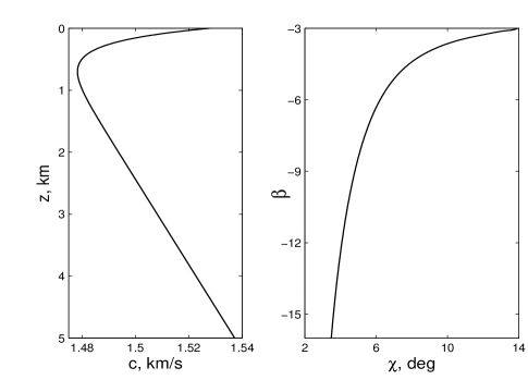
Figure 1: Left panel: sound speed profile used in numerical simulation. Right panel: parameter $\beta$ determined by Eq. (14) vs. ray grazing angle $\chi$ at the sound channel axis $z_{a}=0.7$ km.

Using a standard mode code we evaluated a sound field emitted by a point source set at range $r=0$ and depth $z_{s}=0.3$ km and radiating a sound pulse $s(t)=\exp\left(-\pi t^{2}/T^{2}-2\pi if_{0}t\right)$, where the pulse length $T=0.002$ s and the central frequency $f_{0}=250$ Hz. Only modes with turning points within the water bulk were taken into account.

We analyse sound pulses at points located at depth $z_{r}=z_{s}$ within the range interval from $r=212$ km to $r=312$ km. Signals $u(r,t)$ arriving at these points without reflections from the waveguide boundaries are formed by groups of four eigenrays with $N=4,5,\ldots,8$. In the plot of function $\left|u(r,t)\right|$ shown in Fig. 2 each group of four manifests itself as a fringe. A number next to each fringe indicates the parameter $N$ of eigenrays contributing to the fringe. Since the source and receivers in our example are set at the same depth, in each group of four there are two eigenrays with equal travel times. Therefore fringes corresponding to some groups (with $N=$ 4, 5, and 6) are split into three (not four) more narrow fringes.

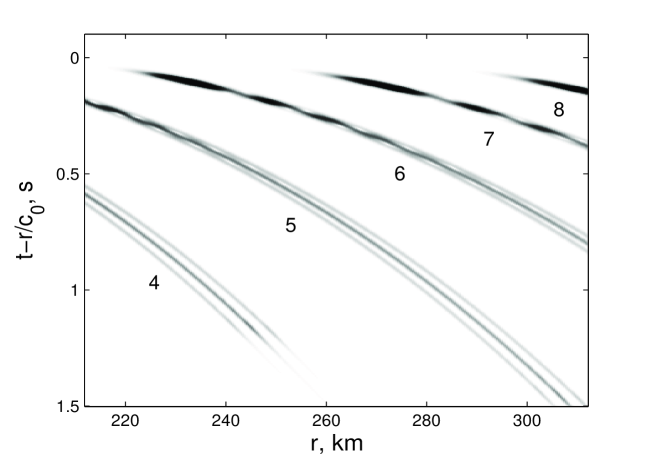
Figure 2: Wave field amplitude $\left|u(r,t)\right|$ at depth $z_{r}=0.3$ km. The wave field is excited by a point source set at depth $z_{s}=z_{r}$ and emitting the short sound pulse $s\left(t\right)$ described in the text. The time is reckoned from $r/c_{0}$, which is the arrival time of an axial ray. Five fringes formed by groups of four eigenrays with $N=4,5,...,8$ are clearly seen.

The interference pattern presented by the autocorrelation function $K(r,\tau)$ is shown in Fig. 3. The fringes formed by pairs of interfering groups of four eigenrays are clearly seen in this plot. A pair of numbers next to each fringe indicates parametes $N$ corresponding to the groups of four forming the fringe. White dashed curves graph interference lines predicted by Eq. (16). Parameters $r_{0}$ and $\tau_{0}$ used in the evaluation of a white curve are the coordinates of a point selected somewhere near the center of the corresponding fringe.

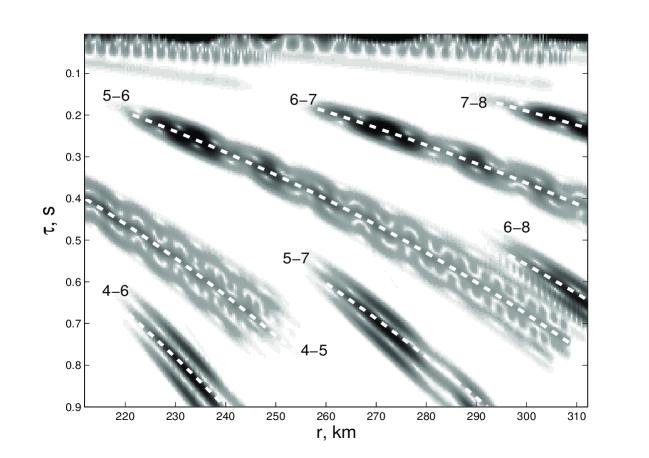
Figure 3: Interference pattern represented by the autocorrelation functions of signals shown in Fig. 2. Seven fringes formed by pairs of groups of four are resolved. Two numbers next to each fringe indicate the numbers of cycles $N$ for a corresponding pair of groups of four. White dashed curves represent interference lines predicted by Eq. (16).

The applicability of Eq. (16) requires the closeness of the action variables of rays forming the interference line. This requirement is satisfied only at long enough ranges where condition (9) is met. Formula (11) is the most accurate for $\Delta N=1$. Figure 3 presents fringes corresponding to $\Delta N=1$ and $\Delta N=2$. Consistent with our expectation, the interference lines predicted by Eq. (16) for $\Delta N=1$ better describe the behavior of fringes than the lines corresponding to $\Delta N=2$.

Observation of fringes associated with the interference lines predicted by Eq. (16) in a non-Chuprov waveguide can be a difficult task. This task is especially complicated in the $\left(r,\omega\right)$ plane, where, according to Eq. (18), each group of four produces a whole set of fringes. The use of a vertical antenna may simplify the resolution of individual fringes. It allows one to diminish the number of terms in sums (5) (6) by selecting waves propagating at grazing angles within a narrow interval. However, the discussion of this issue is beyond the scope of the present paper.

References

- [1] S.D. Chuprov, ‘‘Interference structure of a sound field in a layered ocean,’’ Ocean Acoustics, Modern State (Nauka, Moscow, 1982), pp. 71-91.
- [2] F.B. Jensen, W.A. Kuperman, M.B. Porter, and H. Schmidt. Computational Ocean Acoustics, 2nd edition (Springer Science + Business Media, New York, 2011), Chaps. 2 and 5, pp. 133-139, 337-360, 440-442.
- [3] C.H. Harrison, ’’The relation between the waveguide invariant, multipath impulse response, and ray cycles,’’ J. Acoust. Soc. Am. 129, 2863–2877 (2011).
- [4] G.L. D’Spain and W.A. Kuperman, ‘‘Application of waveguide invariants to analysis of spectrograms from shallow water environments that vary in range and azimuth,’’ J. Acoust. Soc. Am., 106, 2454–2468 (1999).
- [5] K.L. Cockrell and H. Schmidt, ‘‘Robust passive range estimation using the waveguide invariant,’’ J. Acoust. Soc. Am., 127, 2780–2789 (2010).
- [6] R. Goldhahna, G. Hickman, and J. Krolik, ‘‘Waveguide invariant broadband target detection and reverberation estimation,’’ J. Acoust. Soc. Am., 124, 2841–2851 (2011).
- [7] L.M. Zurk and D. Rouseff, ‘‘Striation-based beamforming for active sonar with a horizontal line array,’’ J. Acoust. Soc. Am., 132, EL264–EL270 (2012).
- [8] L.M. Brekhovskikh and Yu.P. Lysanov, Fundamentals of Ocean Acoustics (Springer-Verlag, New York, 2003), Chap. 2.
- [9] A.L. Virovlyanskii, ’’Travel times of acoustic pulses in the ocean,’’ Sov. Phys. Acoust., 31(5), 399–401 (1985).
- [10] A.L. Virovlyansky, ‘‘On general properties of ray arrival sequences in oceanic acoustic waveguides,’’ J. Acoust. Soc. Am. 97, 3180–3183 (1995).
- [11] W. Munk and C. Wunsch, ‘‘Ocean acoustic tomography: rays and modes.’’ Rev. Geophys. and Space. Phys., 21, 1–37 (1983).
- [12] D. Makarov, S. Prants, A. Virovlyansky, and G. Zaslavsky, Ray and wave chaos in ocean acoustics (Word Scientific, New Jersey, 2010), Chaps. 1 and 4, pp. 26-35, 251-268.
- [13] A.L. Virovlyansky, A.Yu. Kazarova, and L.Ya. Lyubavin, ‘‘Statistical description of chaotic rays in a deep water acoustic waveguide,’’ J. Acoust. Soc. Am., 121, pp. 2542–2552 (2007).
- [14] F.J. Beron-Vera and M.G. Brown, ‘‘Underwater acoustic beam dynamics,’’ J. Acoust. Soc. Am., 126, pp. 80–91 (2009).