Contraction Formulas For Kirchhoff And Wiener Indices

Abstract.

We establish several contraction formulas for Kirchhoff index. We relate Kirchhoff index with some other metrized graph invariants. By applying our contraction formulas successively when the graph is a tree, we derive new formulas for Wiener index and obtain some previously known Wiener index formulas with new proofs.

1. Introduction

On a metrized graph $\Gamma$ with set of vertices $V(\Gamma)$ and resistance function $r(x,y)$, the Kirchhoff index $Kf(\Gamma)$ is defined as follows:

$$\begin{split}Kf(\Gamma)=\frac{1}{2}\sum_{p,\,q\in V(\Gamma)}r(p,q).\end{split}$$

For the distance function $d(x,y)$ on $\Gamma$, the Wiener index $W(\Gamma)$ is defined as:

$$\begin{split}W(\Gamma)=\frac{1}{2}\sum_{p,\,q\in V(\Gamma)}d(p,q).\end{split}$$

These definitions of $Kf(\Gamma)$ and $W(\Gamma)$ on a metrized graph $\Gamma$ agree with their usual definitions on a graph. Next, we briefly describe metrized graphs and some notations we use. Then we give a summary of the results we obtained in this paper.

A metrized graph $\Gamma$ is a finite connected graph equipped with a distinguished parametrization of each of its edges. One can consider $\Gamma$ as a one-dimensional manifold except at finitely many branch points , where it looks locally like an n-pointed star. A metrized graph $\Gamma$ can have multiple edges and self-loops. For any given $p\in\Gamma$, the number $\upsilon(p)$ of directions emanating from $p$ will be called the valence of $p$. By definition, there can be only finitely many $p\in\Gamma$ with $\upsilon(p)\not=2$.

For a metrized graph $\Gamma$, we will denote a vertex set for $\Gamma$ by $V(\Gamma)$. We require that $V(\Gamma)$ be finite and non-empty and that $p\in V(\Gamma)$ for each $p\in\Gamma$ if $\upsilon(p)\not=2$. For a given metrized graph $\Gamma$, it is possible to enlarge the vertex set $V(\Gamma)$ by considering additional valence $2$ points as vertices.

For a given metrized graph $\Gamma$ with vertex set $V(\Gamma)$, the set of edges of $\Gamma$ is the set of closed line segments with end points in $V(\Gamma)$. We will denote the set of edges of $\Gamma$ by $E(\Gamma)$. However, if $e_{i}$ is an edge, by $\Gamma-e_{i}$ we mean the graph obtained by deleting the interior of $e_{i}$.

We denote the length of an edge $e_{i}\in E(\Gamma)$ by $L_{i}$, which represents a positive real number. The total length of $\Gamma$, which is denoted by $\ell(\Gamma)$, is given by $\ell(\Gamma)=\sum_{i=1}^{e}L_{i}$.

We use the notation ${\overline{\Gamma}}_{i}$ for the graph obtained by contracting the $i$-th edge $e_{i}$ of a given metrized graph $\Gamma$ to its end points. If $e_{i}\in\Gamma$ has end points $p_{i}$ and $q_{i}$, then in ${\overline{\Gamma}}_{i}$, these points become identical, i.e., $p_{i}=q_{i}$. If $p$ is an end point of an edge $e_{i}$ in $\Gamma$, then by $p$ in $V({\overline{\Gamma}}_{i})$ we mean the vertex, in $V({\overline{\Gamma}}_{i})$, that $p$ is contracted into.

In §2, we briefly describe the voltage and the resistance functions on a metrized graph. We set notations concerning some specific values of these functions and recall some basic results that we use.

In §3, we improved the Kirchhoff index formulas we obtained in [9]. Then we extended the contraction formulas obtained in [8] to bridgeless graphs. Using these results, we give a contraction formula for Kirchhoff index that involves another graph invariant $y(\Gamma)$ (see Equation (1) for the definition of $y(\Gamma)$ and Theorem 3.5 for the contraction formula). This enables us giving lower and upper bounds to Kirchhoff index in terms of $y(\Gamma)$ and applying contraction formulas for Kirchhoff index successively (see Theorem 3.12).

We dealt with tree metrized graphs in §4. Note that the Kirchhoff index is the same as Wiener index for a tree graph. We restate the results we derived for Kirchhoff index in §3 for a tree graph. In this way, we obtain contraction formulas for the Wiener index of a tree graph. Moreover, we obtain new formulas, given in Theorem 4.3 and Theorem 4.6 below, for Wiener index. Our approach enables us to give new proofs of some previously known formulas, Theorem 4.2 and Theorem 4.9, for Wiener index. Then we give various examples that we apply our formulas to compute Wiener indices. At the end of §4, we state two problems. Solution to any of them will be a new proof of a conjecture about Wiener index (see Theorem 4.10 below).

2. Resistance Function $r(x,y)$

In this section, we briefly describe the resistance and the voltage functions on a metrized graph $\Gamma$. We make a review of basic facts about these functions and then set the notation that we use in the rest of the paper.

For any $x$, $y$, $z$ in $\Gamma$, the voltage function $j_{z}(x,y)$ on a metrized graph $\Gamma$ is a symmetric function in $x$ and $y$, which satisfies $j_{x}(x,y)=0$ and $j_{z}(x,y)\geq 0$ for all $x$, $y$, $z$ in $\Gamma$. For each vertex set $V(\Gamma)$, $j_{z}(x,y)$ is continuous on $\Gamma$ as a function of all three variables. For fixed $z$ and $y$ it has the following physical interpretation: If $\Gamma$ is viewed as a resistive electric circuit with terminals at $z$ and $y$, with the resistance in each edge given by its length, then $j_{z}(x,y)$ is the voltage difference between $x$ and $z$, when unit current enters at $y$ and exits at $z$ (with reference voltage $0$ at $z$).

The effective resistance between two points $x,\,y$ of a metrized graph $\Gamma$ is given by $r(x,y)=j_{y}(x,x),$ where $r(x,y)$ is the resistance function on $\Gamma$. The resistance function inherits certain properties of the voltage function. For any $x$, $y$ in $\Gamma$, $r(x,y)$ on $\Gamma$ is a symmetric function in $x$ and $y$, and it satisfies $r(x,x)=0$. For each vertex set $V(\Gamma)$, $r(x,y)$ is continuous on $\Gamma$ as a function of two variables and $r(x,y)\geq 0$ for all $x$, $y$ in $\Gamma$. If a metrized graph $\Gamma$ is viewed as a resistive electric circuit with terminals at $x$ and $y$, with the resistance in each edge given by its length, then $r(x,y)$ is the effective resistance between $x$ and $y$ when unit current enters at $y$ and exits at $x$.

The proofs of the facts mentioned above can be found in [3] and [2, sec 1.5 and sec 6]. The voltage function $j_{z}(x,y)$ and the resistance function $r(x,y)$ are also studied in the articles [1] and [4].

We will denote by $R_{i}$ the resistance between the end points of an edge $e_{i}$ of a graph $\Gamma$ when the interior of the edge $e_{i}$ is deleted from $\Gamma$.

Let $\Gamma$ be a metrized graph with $p\in V(\Gamma)$, and let $e_{i}\in E(\Gamma)$ having end points $p_{i}$ and $q_{i}$. If $\Gamma-e_{i}$ is connected, then $\Gamma$ can be transformed to the graph in Figure 1 by circuit reductions. More details on this fact can be found in the articles [3] and [5, Section 2]. Note that in Figure 1, we have $R_{a_{i},p}=\hat{j}_{p_{i}}(p,q_{i})$, $R_{b_{i},p}=\hat{j}_{q_{i}}(p,p_{i})$, $R_{c_{i},p}=\hat{j}_{p}(p_{i},q_{i})$, where $\hat{j}_{x}(y,z)$ is the voltage function in $\Gamma-e_{i}$. We have $R_{a_{i},p}+R_{b_{i},p}=R_{i}$ for each $p\in\Gamma$.

Remark 2.1.

If $\Gamma-e_{i}$ is not connected, firstly we set $R_{b_{i},p}=R_{i}$ and $R_{a_{i},p}=0$ if $p$ belongs to the component of $\Gamma-e_{i}$ containing $p_{i}$, and we set $R_{a_{i},p}=R_{i}$ and $R_{b_{i},p}=0$ if $p$ belongs to the component of $\Gamma-e_{i}$ containing $q_{i}$. Secondly, we mean $R_{i}\longrightarrow\infty$ in any expression that we use $R_{i}$.

We will use these notations for the rest of the paper. Next, we recall a basic identity concerning these values:

Figure 1. Circuit reduction of $\Gamma$ with reference to an edge $e_{i}$ and a point $p$.

Lemma 2.2.

[7, Lemma 2.11] For any $p$ and $q$ in $V(\Gamma)$,

$$\sum_{e_{i}\in\,E(\Gamma)}\frac{L_{i}(R_{a_{i},p}-R_{b_{i},p})^{2}}{(L_{i}+R_{i})^{2}}=\sum_{e_{i}\in\,E(\Gamma)}\frac{L_{i}(R_{a_{i},q}-R_{b_{i},q})^{2}}{(L_{i}+R_{i})^{2}}.$$

In the rest of the paper, for any metrized graph $\Gamma$ and a fixed vertex $p\in V(\Gamma)$ we will use the following notations, which we first defined in [10] and used also in [9]:

(1) $$\begin{split}y(\Gamma)&=\frac{1}{4}\sum_{e_{i}\,\in E(\Gamma)}\frac{L_{i}R_{i}^{2}}{(L_{i}+R_{i})^{2}}+\frac{3}{4}\sum_{e_{i}\,\in E(\Gamma)}\frac{L_{i}(R_{a_{i},p}-R_{b_{i},p})^{2}}{(L_{i}+R_{i})^{2}},\\ x(\Gamma)&=\sum_{e_{i}\,\in E(\Gamma)}\frac{L_{i}^{2}R_{i}}{(L_{i}+R_{i})^{2}}+\frac{3}{4}\sum_{e_{i}\,\in E(\Gamma)}\frac{L_{i}R_{i}^{2}}{(L_{i}+R_{i})^{2}}-\frac{3}{4}\sum_{e_{i}\,\in E(\Gamma)}\frac{L_{i}(R_{a_{i},p}-R_{b_{i},p})^{2}}{(L_{i}+R_{i})^{2}}.\end{split}$$

Note that $x(\Gamma)$ and $y(\Gamma)$ do not depend on the choice of the vertex $p$ [5, Lemma 2.11]. In [9], we established connections between Kirchhoff index of $\Gamma$ and the invariants $x(\Gamma)$ and $y(\Gamma)$.

When we use $r_{\beta}(x,y)$, we mean the resistance function in the metrized graph $\beta$.

3. Contraction Formulas For Kirchhoff Index

Kirchhoff index of a graph $\Gamma$, $Kf(\Gamma)$, is defined [15] as follows:

(2) $$\begin{split}Kf(\Gamma):=\frac{1}{2}\sum_{p,\,q\in V(\Gamma)}r(p,q).\end{split}$$

The following equality was obtained in [9, page 4038]. It gives a relation between the Kirchhoff index of $\Gamma$ and the Kirchhoff indexes of ${\overline{\Gamma}}_{i}$’s. Although it is a useful formula to understand how Kirchhoff index changes after edge contractions, we can not use it for successive edge contractions because of some technical problems.

(3) $$\begin{split}(v-2)Kf(\Gamma)=\sum_{e_{i}\in E(\Gamma)}\frac{R_{i}}{L_{i}+R_{i}}Kf({\overline{\Gamma}}_{i})+\sum_{e_{i}\in E(\Gamma)}\frac{R_{i}}{L_{i}+R_{i}}\sum_{p\in\,V({\overline{\Gamma}}_{i})}r_{{\overline{\Gamma}}_{i}}(p,\overline{p}_{i}).\end{split}$$

The idea of tracing the value of a graph invariant after successive edge contractions was successfully applied in [8], where we studied the tau constant as an another graph invariant. We want to utilize this idea for Kirchhoff index. To do this, we first need various technical results.

The following lemma is to express $r_{{\overline{\Gamma}}_{i}}(p,\overline{p}_{i})$ in terms of the resistance values on $\Gamma$ that we are more familiar.

Lemma 3.1.

Let $\Gamma$ be a metrized graph, and let $p$ be a vertex of $\Gamma$. For an edge $e_{i}$ of $\Gamma$ with end points $p_{i}$ and $q_{i}$, we have

$$r(p_{i},p)+r(q_{i},p)=2r_{{\overline{\Gamma}}_{i}}(p,\overline{p}_{i})+\frac{L_{i}R_{i}}{L_{i}+R_{i}}-2\frac{L_{i}R_{a_{i},p}R_{b_{i},p}}{R_{i}(L_{i}+R_{i})}.$$

Proof.

We prove this in two cases.

Case I: $e_{i}$ is not a bridge.

From [7, Section 2], we have

(4) $$\begin{split}r(p_{i},p)=\frac{(L_{i}+R_{b_{i},p})R_{a_{i},p}}{L_{i}+R_{i}}+R_{c_{i},p},\quad\text{and}\quad r(q_{i},p)=\frac{(L_{i}+R_{a_{i},p})R_{b_{i},p}}{L_{i}+R_{i}}+R_{c_{i},p}.\end{split}$$

Thus,

(5) $$\begin{split}r(p_{i},p)+r(q_{i},p)=\frac{L_{i}R_{i}}{L_{i}+R_{i}}+2\frac{R_{a_{i},p}R_{b_{i},p}}{L_{i}+R_{i}}+2R_{c_{i},p}.\end{split}$$

On the other hand, from [10, Equation 17] we have

(6) $$\begin{split}r_{{\overline{\Gamma}}_{i}}(p,\overline{p}_{i})=\frac{R_{a_{i},p}R_{b_{i},p}}{R_{i}}+R_{c_{i},p}.\end{split}$$

Thus, the result follows from Equations (5) and (6) in this case.

Case II: $e_{i}$ is a bridge.

If $p$ belongs to the component of $\Gamma-e_{i}$ containing $p_{i}$, we have $r(p_{i},p)+r(q_{i},p)=L_{i}+2r(p_{i},p)$ and $r_{{\overline{\Gamma}}_{i}}(p,\overline{p}_{i})=r(p_{i},p)$.

If $p$ belongs to the component of $\Gamma-e_{i}$ containing $q_{i}$, we have $r(p_{i},p)+r(q_{i},p)=L_{i}+2r(q_{i},p)$ and $r_{{\overline{\Gamma}}_{i}}(p,\overline{p}_{i})=r(q_{i},p)$.

Now, we note that $\frac{L_{i}R_{i}}{L_{i}+R_{i}}\longrightarrow 0$ and $\frac{L_{i}R_{a_{i},p}R_{b_{i},p}}{R_{i}(L_{i}+R_{i})}\longrightarrow 0$ because of Remark 2.1.

Thus, the result follows in this case, too.

∎

Now, we can substitute the value of $r_{{\overline{\Gamma}}_{i}}(p,\overline{p}_{i})$ obtained from Lemma 3.1 into the formula given in Equation (3). In this way, we derive a new formula for Kirchhoff index.

Lemma 3.2.

Let $\Gamma$ be a metrized graph. We have

$$\begin{split}2(v-2)Kf(\Gamma)&=2\sum_{e_{i}\in E(\Gamma)}\frac{R_{i}}{L_{i}+R_{i}}Kf({\overline{\Gamma}}_{i})+2v\sum_{e_{i}\in E(\Gamma)}\frac{L_{i}R_{a_{i},p}R_{b_{i},p}}{(L_{i}+R_{i})^{2}}-v\sum_{e_{i}\in E(\Gamma)}\frac{L_{i}R_{i}^{2}}{(L_{i}+R_{i})^{2}}\\ &\qquad+\sum_{p\in V(\Gamma)}\sum_{e_{i}\in E(\Gamma)}\frac{R_{i}}{L_{i}+R_{i}}(r(p_{i},p)+r(q_{i},p)).\end{split}$$

Proof.

Since $R_{i}=R_{a_{i},p}+R_{b_{i},p}$ for any $p\in V(\Gamma)$, we have

(7) $$\begin{split}\sum_{e_{i}\in E(\Gamma)}\frac{L_{i}R_{i}^{2}}{(L_{i}+R_{i})^{2}}=\sum_{e_{i}\in E(\Gamma)}\frac{L_{i}(R_{a_{i},p}-R_{b_{i},p})^{2}}{(L_{i}+R_{i})^{2}}+4\sum_{e_{i}\in E(\Gamma)}\frac{L_{i}R_{a_{i},p}R_{b_{i},p}}{(L_{i}+R_{i})^{2}}.\end{split}$$

We note that the left hand side of Equation (7) is independent of the choice of the vertex $p$. Likewise, the first term at the right side of Equation (7) is independent of $p$ because of Lemma 2.2. Therefore,

(8) $$\begin{split}\sum_{e_{i}\in E(\Gamma)}\frac{L_{i}R_{a_{i},p}R_{b_{i},p}}{(L_{i}+R_{i})^{2}}=\sum_{e_{i}\in E(\Gamma)}\frac{L_{i}R_{a_{i},q}R_{b_{i},q}}{(L_{i}+R_{i})^{2}},\qquad\text{for any vertices $p$ and $q$.}\end{split}$$

Now, we first multiply the equality in Lemma 3.1 by $\frac{R_{i}}{L_{i}+R_{i}}$ and take the summation of the resulting equality over all edges $e_{i}$ in $E(\Gamma)$. Then we take the summation of the equality obtained over all vertices $p$ in $V(\Gamma)$. Finally, the result follows from Equation (8), Equation (3) and the equality we derived. ∎

Now, our goal is to simplify the formula we obtained in Lemma 3.2. First, we improve a result we derived previously.

The following lemma with the condition that $\Gamma$ is a bridgeless metrized graph was proved in [10, Lemma 3.10]. We note that this condition is not necessary.

Lemma 3.3.

Let $\Gamma$ be a metrized graph, and let $p_{i}$ and $q_{i}$ be the end points of $e_{i}\in E(\Gamma)$. For any $p\in V(\Gamma)$, we have

$$\begin{split}\sum_{e_{i}\in\,E(\Gamma)}\frac{L_{i}(R_{a_{i},p}-R_{b_{i},p})^{2}}{(L_{i}+R_{i})^{2}}&=\sum_{e_{i}\in\,E(\Gamma)}\frac{L_{i}}{L_{i}+R_{i}}\big{(}r(p_{i},p)+r(q_{i},p)\big{)}-\sum_{q\in V(\Gamma)}(\upsilon(q)-2)r(p,q)\\ &=2\sum_{q\in V(\Gamma)}r(p,q)-\sum_{e_{i}\in\,E(\Gamma)}\frac{R_{i}}{L_{i}+R_{i}}\big{(}r(p_{i},p)+r(q_{i},p)\big{)}.\end{split}$$

Proof.

The proof is almost the same as the proof of [10, Lemma 3.10]. The only additional work is to use the following facts for edges that are bridges (edges whose removal disconnects the graph).

Figure 2. $\Gamma$ with $x\in e_{i}$, where $e_{i}$ is a bridge.

Let $e_{i}\in E(\Gamma)$ be a bridge, and let $p\in V(\Gamma)$. Suppose $x\in e_{i}$ is as in Figure 2 and that $e_{i}$ has end points $p_{i}$ and $q_{i}$. If $p$ belongs to the component of $\Gamma-e_{i}$ containing $p_{i}$, we have

(9) $$\begin{split}r(p,x)=r(p,p_{i})+x,\qquad\frac{d}{dx}r(p,x)=1,\quad\text{and }r(p,p_{i})-r(p,q_{i})=-L_{i}.\end{split}$$

If $p$ belongs to the component of $\Gamma-e_{i}$ containing $q_{i}$, we have

(10) $$\begin{split}r(p,x)=r(p,q_{i})+L_{i}-x,\qquad\frac{d}{dx}r(p,x)=-1\quad\text{and }r(p,p_{i})-r(p,q_{i})=L_{i}.\end{split}$$

Thus, in any case $\frac{d^{2}}{dx^{2}}r(p,x)=0$ if $x$ belongs to a bridge.

We note that [10, Lemma 3.6], [10, Equation (14)] and [10, Proposition 3.9] are valid for metrized graphs with possibly bridges.

If we consider Remark 2.1 along with Equations (9) and (10), the proof of [10, Lemma 3.10] can be extended to the case $\Gamma$ with bridges. ∎

Lemma 3.3 is crucial for our purposes.

Lemma 3.4.

For any metrized graph $\Gamma$, we have

$$\begin{split}4Kf(\Gamma)=v\cdot\sum_{e_{i}\in\,E(\Gamma)}\frac{L_{i}(R_{a_{i},p}-R_{b_{i},p})^{2}}{(L_{i}+R_{i})^{2}}+\sum_{e_{i}\in\,E(\Gamma)}\frac{R_{i}}{L_{i}+R_{i}}\sum_{p\in V(\Gamma)}\big{(}r(p_{i},p)+r(q_{i},p)\big{)}.\end{split}$$

Proof.

First, we take summation of the second equality in Lemma 3.3 over all vertices $p\in V(\Gamma)$:

$$\begin{split}\sum_{p\in V(\Gamma)}\sum_{e_{i}\in\,E(\Gamma)}\frac{L_{i}(R_{a_{i},p}-R_{b_{i},p})^{2}}{(L_{i}+R_{i})^{2}}=2\sum_{p,\,q\in V(\Gamma)}r(p,q)-\sum_{e_{i}\in\,E(\Gamma)}\frac{R_{i}}{L_{i}+R_{i}}\sum_{p\in V(\Gamma)}\big{(}r(p_{i},p)+r(q_{i},p)\big{)}.\end{split}$$

Then the result follows from this equality, Lemma 2.2 and the definition of $Kf(\Gamma)$. ∎

After having various technical lemmas, we can state our first main result. It describes the relation between the Kirchhoff index of $\Gamma$ and the Kirchhoff indexes of each of ${\overline{\Gamma}}_{i}$ that are obtained by contraction of $e_{i}\in E(\Gamma)$:

Theorem 3.5.

Let $\Gamma$ be a metrized graph with at least $4$ vertices. Then we have

$$(v-4)Kf(\Gamma)=\sum_{e_{i}\in E(\Gamma)}\frac{R_{i}}{L_{i}+R_{i}}Kf({\overline{\Gamma}}_{i})-v\cdot y(\Gamma).$$

Proof.

We first subtract the equality given in Lemma 3.4 from the equality given in Lemma 3.2. Then the proof follows from Equation (7) and Equation (1). ∎

Next, we have another formula for Kirchhoff index.

Proposition 3.6.

For any metrized graph $\Gamma$ with $v$ vertices, we have

$$2Kf(\Gamma)=v\cdot y(\Gamma)+\sum_{e_{i}\in E(\Gamma)}\frac{R_{i}}{L_{i}+R_{i}}\sum_{p\in\,V({\overline{\Gamma}}_{i})}r_{{\overline{\Gamma}}_{i}}(p,\overline{p}_{i}).$$

Proof.

The result is obtained by subtracting the formula in Theorem 3.5 from Equation (3). ∎

Note that Theorem 3.5 is more advantageous to work with than Equation (3), because we studied the term $y(\Gamma)$ previously [8] and showed that it has various properties.

Our goal for the rest of this section is to apply the contraction formula given in Theorem 3.5 successively. To do this, we need the contraction formula for $y(\Gamma)$ for any metrized graph $\Gamma$ (see Theorem 3.9 below). The contraction formula of $y(\Gamma)$ for bridgeless metrized graphs was shown in [8, Theorem 4.12]. First, we need some preparatory work.

The following theorem was given in [9, Theorem 4.8]. Note that we don’t need the condition bridgeless as explained in the paragraph before the theorem in that paper (and as its proof shows). That is, we can give [9, Theorem 4.8] with a minor correction in its statement as follows:

Theorem 3.7.

Let $\Gamma$ be a metrized graph. For any two vertices $p$ and $q$, we have

$$\begin{split}(v-2)r(p,q)=\sum_{e_{i}\in E(\Gamma)}\frac{R_{i}}{L_{i}+R_{i}}r_{{\overline{\Gamma}}_{i}}(p,q).\end{split}$$

Next, we apply Theorem 3.7 to the sum of effective resistances along with all edges. Let

$$r(\Gamma):=\sum_{e_{i}\in E(\Gamma)}\frac{L_{i}R_{i}}{L_{i}+R_{i}}.$$

Note that $r(p_{i},q_{i})=\frac{L_{i}R_{i}}{L_{i}+R_{i}}$ for any edge $e_{i}$ with end points $p_{i}$ and $q_{i}$.

Theorem 3.8.

Let $\Gamma$ be a metrized graph. Then, we have

$$\begin{split}(v-2)r(\Gamma)=\sum_{e_{i}\in E(\Gamma)}\frac{R_{i}}{L_{i}+R_{i}}r({\overline{\Gamma}}_{i}).\end{split}$$

Proof.

Let $e_{j}$ be an edge with end points $p_{j}$ and $q_{j}$. Applying Theorem 3.7 to the vertices $p_{j}$ and $q_{j}$ gives

$$\begin{split}(v-2)r(p_{j},q_{j})=\sum_{e_{i}\in E(\Gamma)}\frac{R_{i}}{L_{i}+R_{i}}r_{{\overline{\Gamma}}_{i}}(p_{j},q_{j}).\end{split}$$

where $v$ is the number of vertices in $\Gamma$. Now, if we take the summation of above equality over all edges $e_{j}$ in $\Gamma$ and use the definition of $r(\Gamma)$, we obtain

$$\begin{split}(v-2)r(\Gamma)&=\sum_{e_{i}\in E(\Gamma)}\frac{R_{i}}{L_{i}+R_{i}}\sum_{e_{j}\in E(\Gamma)}r_{{\overline{\Gamma}}_{i}}(p_{j},q_{j})\\ &=\sum_{e_{i}\in E(\Gamma)}\frac{R_{i}}{L_{i}+R_{i}}\sum_{e_{j}\in E({\overline{\Gamma}}_{i})}r_{{\overline{\Gamma}}_{i}}(p_{j},q_{j}),\qquad\text{since $r_{{\overline{\Gamma}}_{i}}(p_{i},q_{i})=0$}.\\ &=\sum_{e_{i}\in E(\Gamma)}\frac{R_{i}}{L_{i}+R_{i}}r({\overline{\Gamma}}_{i}).\end{split}$$

This gives what we want to show. ∎

Note that Theorem 3.8 for bridgeless metrized graphs was given in [8, Corollary 4.13]. But we show here that it holds for any metrized graphs possibly with bridges.

Similarly, the following theorem for bridgeless metrized graphs was given in [8, Theorem 4.12].

Theorem 3.9.

Let $\Gamma$ be a metrized graph with $v$ vertices. Then we have

$$(v-2)x(\Gamma) =\sum_{e_{i}\in E(\Gamma)}\frac{R_{i}}{L_{i}+R_{i}}x({\overline{\Gamma}}_{i}), \text{ and }\quad(v-2)y(\Gamma) =\sum_{e_{i}\in E(\Gamma)}\frac{R_{i}}{L_{i}+R_{i}}y({\overline{\Gamma}}_{i}).$$

Proof.

Let $B(\Gamma)=\{e_{i_{1}},\,e_{i_{2}},\dots,e_{i_{t}}\}$ be the set of bridges in $\Gamma$. Let $\beta$ be the metrized graph obtained from $\Gamma$ by contracting all bridges in $\Gamma$.

We first note that if $e_{i}$ is a bridge, using Remark 2.1 we obtain $\frac{L_{i}^{2}R_{i}}{(L_{i}+R_{i})^{2}}\longrightarrow 0$, $\frac{L_{i}R_{i}^{2}}{(L_{i}+R_{i})^{2}}\longrightarrow L_{i}$ and $\frac{L_{i}(R_{a_{i},p}-R_{b_{i},p})^{2}}{(L_{i}+R_{i})^{2}}\longrightarrow L_{i}$. Therefore, considering the definition of $x(\Gamma)$ in Equation (1) we conclude that bridges in $\Gamma$ does not contribute to $x(\Gamma)$. Moreover, $R_{j}(\Gamma)=R_{j}(\beta)$ if $e_{j}$ is not a bridge. Hence,

(11) $$\begin{split}&x(\Gamma)=x({\overline{\Gamma}}_{i})\quad\text{when $e_{i}$ is a bridge, and so }x(\Gamma)=x(\beta).\\ &x({\overline{\Gamma}}_{i})=x(\overline{\beta}_{i})\quad\text{when $e_{i}$ is not a bridge}.\end{split}$$

We use Equation (11) and Remark 2.1 in the second equality below:

(12) $$\begin{split}\sum_{e_{i}\in E(\Gamma)}\frac{R_{i}}{L_{i}+R_{i}}x({\overline{\Gamma}}_{i})&=\sum_{e_{i}\in E(\Gamma)-B(\Gamma)}\frac{R_{i}}{L_{i}+R_{i}}x({\overline{\Gamma}}_{i})+\sum_{e_{i}\in B(\Gamma)}\frac{R_{i}}{L_{i}+R_{i}}x({\overline{\Gamma}}_{i})\\ &=\sum_{e_{i}\in E(\Gamma)-B(\Gamma)}\frac{R_{i}}{L_{i}+R_{i}}x(\beta)+\sum_{e_{i}\in B(\Gamma)}x(\beta),\\ &=(v-t-2)x(\beta)+t\cdot x(\beta),\qquad\text{using \cite[cite]{[\@@bibref{}{C5}{}{}, Theorem 4.12]} for $\beta$.}\\ &=(v-2)x(\Gamma),\qquad\text{by using Equation~{}(\ref{eqn contraction xa})}.\end{split}$$

This proves the first equality in the theorem. Next, we prove the second equality. We first note that $r(\Gamma)=x(\Gamma)+y(\Gamma)$ for any metrized graph $\Gamma$.

On one hand, by Theorem 3.8 we have

(13) $$\begin{split}(v-2)r(\Gamma)=\sum_{e_{i}\in E(\Gamma)}\frac{R_{i}}{L_{i}+R_{i}}r({\overline{\Gamma}}_{i})=\sum_{e_{i}\in E(\Gamma)}\frac{R_{i}}{L_{i}+R_{i}}\big{(}x({\overline{\Gamma}}_{i})+y({\overline{\Gamma}}_{i})\big{)}.\end{split}$$

On the other hand, by the first equality that we just proved for $x(\Gamma)$

$$(v-2)r(\Gamma)=(v-2)x(\Gamma)+(v-2)y(\Gamma)=(v-2)y(\Gamma)+\sum_{e_{i}\in E(\Gamma)}\frac{R_{i}}{L_{i}+R_{i}}x({\overline{\Gamma}}_{i}).$$

Thus, the second equality in the theorem follows from this equality and Equation (13). ∎

When the number of vertices is $2$ or $3$, we know the exact relation between $Kf(\Gamma)$ and $y(\Gamma)$.

Corollary 3.10.

For any metrized graph $\Gamma$ with $v$ vertices. Then we have

$$Kf(\Gamma)=y(\Gamma),\quad\text{if $v=2$}.\qquad Kf(\Gamma)=2y(\Gamma),\quad\text{if $v=3$}.$$

Proof.

When $v=2$, ${\overline{\Gamma}}_{i}$ has only one vertex. In this case, $Kf({\overline{\Gamma}}_{i})=0$ for each edge $e_{i}$. Then Theorem 3.5 gives that $Kf(\Gamma)=y(\Gamma)$.

When $v=3$, ${\overline{\Gamma}}_{i}$ has two vertices, so we have $Kf({\overline{\Gamma}}_{i})=y({\overline{\Gamma}}_{i})$ by the first equality. Thus, Theorem 3.5 gives

$$-Kf(\Gamma)=\sum_{e_{i}\in E(\Gamma)}\frac{R_{i}}{L_{i}+R_{i}}Kf({\overline{\Gamma}}_{i})-3\cdot y(\Gamma)=\sum_{e_{i}\in E(\Gamma)}\frac{R_{i}}{L_{i}+R_{i}}y({\overline{\Gamma}}_{i})-3\cdot y(\Gamma)=-2y(\Gamma),$$

where the last equality follows from Theorem 3.9. This completes the proof. ∎

For any integer $1\leq k\leq v-2$, if an edge $e_{i_{k}}$ is not a self loop in ${\overline{\Gamma}}_{i_{1},i_{2},\dots,i_{k-1}}$, then $\#(V({\overline{\Gamma}}_{i_{1},i_{2},\dots,i_{k}}))=\#(V({\overline{\Gamma}}_{i_{1},i_{2},\dots,i_{k-1}}))-1$. We call ${\overline{\Gamma}}_{i_{1},i_{2},\dots,i_{k}}$ be an admissible contraction of $\Gamma$, if it is obtained from $\Gamma$ by contracting edges with distinct end points at each step. We have $\#(V({\overline{\Gamma}}_{i_{1},i_{2},\dots,i_{k}}))=v-k$ iff $V({\overline{\Gamma}}_{i_{1},i_{2},\dots,i_{k}})$ is an admissible contraction of $\Gamma$. Note that we have $\frac{R_{i}}{L_{i}+R_{i}}=0$ for a self loop, so contraction of self loops can be neglected in contraction identities. Therefore, we restrict ourselves to the admissible contractions only.

Now, we successively apply the contraction identity given in Theorem 3.9 as follows:

Theorem 3.11.

Let $\Gamma$ be metrized graph with $v\geq 3$ vertices, and let $k$ be an integer with $1\leq k\leq v-2$. For admissible contractions, we have

$$\begin{split}\frac{(v-2)!}{(v-k-2)!}x(\Gamma)&=\sum_{\begin{subarray}{c}e_{i_{1}}\in\\ E(\Gamma)\end{subarray}}\frac{R_{i_{1}}}{L_{i_{1}}+R_{i_{1}}}\sum_{\begin{subarray}{c}e_{i_{2}}\in\\ E({\overline{\Gamma}}_{i_{1}})\end{subarray}}\frac{R_{i_{2}}}{L_{i_{2}}+R_{i_{2}}}\;\dots\sum_{\begin{subarray}{c}e_{i_{k}}\in\\ E({\overline{\Gamma}}_{i_{1},\dots,i_{k-1}})\end{subarray}}\frac{R_{i_{k}}}{L_{i_{k}}+R_{i_{k}}}x({\overline{\Gamma}}_{i_{1},\dots,i_{k}}),\\ \frac{(v-2)!}{(v-k-2)!}y(\Gamma)&=\sum_{\begin{subarray}{c}e_{i_{1}}\in\\ E(\Gamma)\end{subarray}}\frac{R_{i_{1}}}{L_{i_{1}}+R_{i_{1}}}\sum_{\begin{subarray}{c}e_{i_{2}}\in\\ E({\overline{\Gamma}}_{i_{1}})\end{subarray}}\frac{R_{i_{2}}}{L_{i_{2}}+R_{i_{2}}}\;\dots\sum_{\begin{subarray}{c}e_{i_{k}}\in\\ E({\overline{\Gamma}}_{i_{1},\dots,i_{k-1}})\end{subarray}}\frac{R_{i_{k}}}{L_{i_{k}}+R_{i_{k}}}y({\overline{\Gamma}}_{i_{1},\dots,i_{k}}).\end{split}$$

Proof.

We have $\frac{R_{i_{j}}}{L_{i_{j}}+R_{i_{j}}}=0$ for an edge $e_{i_{j}}$ that is a self loop. Thus, contraction of self loops does not contribute to sums in contraction identities. Applying Theorem 3.9 inductively gives the result. ∎

Note that Theorem 3.11 generalizes the similar results in [8] to any metrized graph.

Next, we take the advantage of the contraction formula to derive Theorem 3.12 which is our second main result. It describes how Kirchhoff index changes under successive edge contractions.

Theorem 3.12.

Let $\Gamma$ be metrized graph with $v\geq 5$ vertices. and let $k$ be an integer with $1\leq k\leq v-4$. For admissible contractions, we have

$$\begin{split}Kf(\Gamma)&=\frac{(v-4-k)!}{(v-4)!}\sum_{\begin{subarray}{c}e_{i_{1}}\in\\ E(\Gamma)\end{subarray}}\frac{R_{i_{1}}}{L_{i_{1}}+R_{i_{1}}}\sum_{\begin{subarray}{c}e_{i_{2}}\in\\ E({\overline{\Gamma}}_{i_{1}})\end{subarray}}\frac{R_{i_{2}}}{L_{i_{2}}+R_{i_{2}}}\;\dots\sum_{\begin{subarray}{c}e_{i_{k}}\in\\ E({\overline{\Gamma}}_{i_{1},\dots,i_{k-1}})\end{subarray}}\frac{R_{i_{k}}}{L_{i_{k}}+R_{i_{k}}}Kf({\overline{\Gamma}}_{i_{1},\dots,i_{k}})\\ &\qquad-\frac{\big{(}v^{2}-(k+2)v+k-1\big{)}k}{(v-k-2)(v-k-3)}y(\Gamma).\end{split}$$

In particular, if $k=v-4$, we have

$$\begin{split}Kf(\Gamma)&=\frac{1}{(v-4)!}\sum_{\begin{subarray}{c}e_{i_{1}}\in\\ E(\Gamma)\end{subarray}}\frac{R_{i_{1}}}{L_{i_{1}}+R_{i_{1}}}\sum_{\begin{subarray}{c}e_{i_{2}}\in\\ E({\overline{\Gamma}}_{i_{1}})\end{subarray}}\frac{R_{i_{2}}}{L_{i_{2}}+R_{i_{2}}}\;\dots\sum_{\begin{subarray}{c}e_{i_{v-4}}\in\\ E({\overline{\Gamma}}_{i_{1},\dots,i_{v-5}})\end{subarray}}\frac{R_{i_{v-4}}}{L_{i_{v-4}}+R_{i_{v-4}}}Kf({\overline{\Gamma}}_{i_{1},\dots,i_{v-4}})\\ &\qquad-\frac{(3v-5)(v-4)}{2}y(\Gamma).\end{split}$$

Proof.

The proof follows by successive application of Theorem 3.5 for each $Kf({\overline{\Gamma}}_{i_{1},\dots,i_{k}})$ and Theorem 3.9 for each $y({\overline{\Gamma}}_{i_{1},\dots,i_{k}})$. One should be careful about determining the coefficient of $y(\Gamma)$ after each contraction step. Note that we can compute the coefficient of $y(\Gamma)$ at the $k$-th contraction step with the help of the following identity:

$$\frac{v}{v-4}+\sum_{i=1}^{k-1}\frac{v-i}{v-4-i}\prod_{j=1}^{i}\frac{v-1-j}{v-3-j}=\frac{\big{(}v^{2}-(k+2)v+k-1\big{)}k}{(v-k-2)(v-k-3)}.$$

∎

Note that ${\overline{\Gamma}}_{i_{1},\dots,i_{v-4}}$ has $4$ vertices. Therefore, it is important to know the relation between $Kf(\Gamma)$ and $y(\Gamma)$ when $\Gamma$ has $4$ edges to derive further conclusions from Theorem 3.12. Although the exact relation as in Corollary 3.10 is not possible in general, we can have upper and lower bounds of $Kf(\Gamma)$ in terms of $y(\Gamma)$. This is what we show below. First, we recall some facts.

Suppose the set of vertices for an admissible contraction ${\overline{\Gamma}}_{i_{1},i_{2},\dots,i_{v-2}}$ of $\Gamma$ is $\{p^{\prime},q^{\prime}\}$. Let $m$ vertices of $\Gamma$ are contracted into $p^{\prime}$ and the remaining $k$ vertices are contracted into $q^{\prime}$. Then both $m$ and $k$ are positive integers with $m+k=v$, where $v$ is the number of vertices in $\Gamma$.

Next, we state a corollary to Theorem 3.11. It generalizes the relevant result from [8] to any metrized graph possibly with bridges.

Corollary 3.13.

Let $\Gamma$ be metrized graph with $v\geq 3$ vertices. For admissible contractions ${\overline{\Gamma}}_{i_{1},\dots,i_{v-2}}$, we have

$$(v-2)!y(\Gamma)=\sum_{\begin{subarray}{c}e_{i_{1}}\in\\ E(\Gamma)\end{subarray}}\frac{R_{i_{1}}}{L_{i_{1}}+R_{i_{1}}}\sum_{\begin{subarray}{c}e_{i_{2}}\in\\ E({\overline{\Gamma}}_{i_{1}})\end{subarray}}\frac{R_{i_{2}}}{L_{i_{2}}+R_{i_{2}}}\;\dots\sum_{\begin{subarray}{c}e_{i_{v-2}}\in\\ E({\overline{\Gamma}}_{i_{1},\dots,i_{v-3}})\end{subarray}}\frac{R_{i_{v-2}}}{L_{i_{v-2}}+R_{i_{v-2}}}r_{{\overline{\Gamma}}_{i_{1},\dots,i_{v-2}}}(p^{\prime},q^{\prime}).$$

Proof.

First we note that $y({\overline{\Gamma}}_{i_{1},\dots,i_{v-2}})=r_{{\overline{\Gamma}}_{i_{1},\dots,i_{v-2}}}(p^{\prime},q^{\prime})$ by the proof of [8, Proposition 5.8].

Then the result follows from Theorem 3.11 with $k=v-2$. ∎

We recall another contraction formula for the Kirchhoff index.

Lemma 3.14.

[9, Lemma 5.2] Let $\Gamma$ be a metrized graph with $v$ vertices, and let $m$ and $k$ be defined as above. For any admissible contraction ${\overline{\Gamma}}_{i_{1},i_{2},\dots,i_{v-2}}$, we have

$$Kf(\Gamma)=\frac{1}{(v-2)!}\sum_{\begin{subarray}{c}e_{i_{1}}\in\\ E(\Gamma)\end{subarray}}\frac{R_{i_{1}}}{L_{i_{1}}+R_{i_{1}}}\dots\sum_{\begin{subarray}{c}e_{i_{v-2}}\in\\ E({\overline{\Gamma}}_{i_{1},\dots,i_{v-3}})\end{subarray}}\frac{R_{i_{v-2}}}{L_{i_{v-2}}+R_{i_{v-2}}}m\cdot k\cdot r_{{\overline{\Gamma}}_{i_{1},\dots,i_{v-2}}}(p^{\prime},q^{\prime}).$$

The following upper bound was given in [9, Equation 21] for regular graphs that are bridgeless. Now, we have it without any restriction on $\Gamma$:

Corollary 3.15.

For any metrized graph $\Gamma$ with $v$ vertices, we have

$$Kf(\Gamma)\leq\frac{v^{2}}{4}y(\Gamma).$$

Proof.

When $m+k=v$ for any two positive integers $m$ and $k$, the maximum of $m\cdot k$ is at most $\frac{v^{2}}{4}$. Then the proof follows from Lemma 3.14 and Corollary 3.13. ∎

Lemma 3.16.

Let $\Gamma$ be a metrized graph with $4$ vertices. Then we have

$$3y(\Gamma)\leq Kf(\Gamma)\leq 4y(\Gamma).$$

Proof.

We apply the contraction formula given in Lemma 3.14 to $\Gamma$. Since $m+k=4$ and both $m$ and $k$ are positive integers, we either have $m\cdot k=3$ or $m\cdot k=4$. Thus, the inequalities in the lemma follows from Corollary 3.13. ∎

Now, using Lemma 3.16 for ${\overline{\Gamma}}_{i_{1},\dots,i_{v-4}}$, Theorem 3.12 and Theorem 3.11 with $k=v-4$, we derive the following proposition:

Proposition 3.17.

For any metrized graph with $v\geq 4$, we have

$$(v-1)y(\Gamma)\leq Kf(\Gamma)\leq\frac{v^{2}-3v+4}{2}y(\Gamma).$$

We note that when $v\geq 5$ Corollary 3.15 gives better upper bounds then Proposition 3.17.

Next, we give an example to illustrate how the contraction formula in Theorem 3.12 can be used.

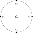
Figure 3. Circle graph with $4$ vertices

Example I: Let $C_{v}$ be the circle graph with $v$ vertices and $v$ edges. Figure 3 illustrates $C_{4}$. Suppose each edge length of the metrized graph $\Gamma=C_{v}$ is equal to $1$. Then $\ell(C_{v})=v$, and we have $Kf(C_{4})=5$ by direct computation. Moreover, $\tau(\Gamma)=\frac{1}{12}\ell(C_{v})$ by [7, Corollary 2.17], $\tau(\Gamma)=\frac{1}{12}\ell(C_{v})-\frac{x(\Gamma)-y(\Gamma)}{6}$ by [8, Equation 20], $x(\Gamma)+y(\Gamma)=\frac{v-1}{v}\ell(C_{v})$ by [9, Lemma 6.3]. Thus, $x(\Gamma)=y(\Gamma)=\frac{v-1}{2}$.

Since ${\overline{\Gamma}}_{i_{1},\dots,i_{v-4}}=C_{4}$ for every admissible contraction of $\Gamma$ in this case, applying Theorem 3.12 with $k=v-4$ gives $Kf(C_{v})=\frac{v(v^{2}-1)}{12}$. This agrees with the result obtained in [17, Equation (5)].

4. Trees, When Kirchhoff Index is Wiener Index

In this section, we restrict ourselves to tree metrized graphs. A tree graph is a connected graph with no cycle. That is, each edge in a tree graph is a bridge. We rewrite many of the results from §3 for the tree metrized graphs. In this way, we obtain new formulas for the Wiener index of tree graphs, and give new proofs to some previously know formulas for Wiener index.

Let $d(p,q)$ denote the distance between the vertices $p$ and $q$ in $V(\Gamma)$. Then the Wiener index of $\Gamma$ is defined as follows (see [11, page 211] and the references therein):

$$W(\Gamma):=\frac{1}{2}\sum_{p,\,q\in V(\Gamma)}d(p,q).$$

When $\Gamma$ is a tree, $d(p,q)=r(p,q)$ for each vertices $p$ and $q$, where $r(x,y)$ is the resistance function on $\Gamma$. Therefore,

(14) $$\begin{split}W(\Gamma)=Kf(\Gamma)\quad\text{if $\Gamma$ is a tree}.\end{split}$$

When $\Gamma$ is a tree, Lemma 3.3 can be restated as follows

Lemma 4.1.

Let $\Gamma$ be a metrized graph that is a tree with $v$ vertices. For any $p\in V(\Gamma)$, we have

$$\ell(\Gamma)=\sum_{q\in V(\Gamma)}(2-\upsilon(q))r(p,q).$$

In particular, if each edge length is equal to $1$, we have

$$v-1=\sum_{q\in V(\Gamma)}(2-\upsilon(q))r(p,q).$$

Proof.

Each edge is a bridge in $\Gamma$ as it is a tree. Thus, we have $(R_{a_{i},p}-R_{b_{i},p})^{2}=R_{i}^{2}$ for each edge in $\Gamma$, and so $\frac{L_{i}(R_{a_{i},p}-R_{b_{i},p})^{2}}{(L_{i}+R_{i})^{2}}=\frac{L_{i}R_{i}^{2}}{(L_{i}+R_{i})^{2}}$. We have $\frac{L_{i}R_{i}^{2}}{(L_{i}+R_{i})^{2}}\longrightarrow L_{i}$ and $\frac{L_{i}}{L_{i}+R_{i}}\longrightarrow 0$ as $R_{i}\longrightarrow\infty$. Therefore, the first equality in the lemma follows from the first equality given in Lemma 3.3. When $L_{i}=1$ for every $e_{i}\in E(\Gamma)$, the second equality in the lemma is obtained by using the fact that $\ell(\Gamma)=e=v-1$, where $e$ is the number of edges of $\Gamma$. ∎

Theorem 4.2.

Let $\Gamma$ be a metrized graph that is a tree with $v$ vertices. Then we have

$$W(\Gamma)=\frac{1}{4}\Big{[}v\cdot\ell(\Gamma)+\sum_{p,\,\,q\in V(\Gamma)}\upsilon(q)r(p,q)\Big{]}.$$

In particular, if each edge length is equal to $1$, we have

$$W(\Gamma)=\frac{1}{4}\Big{[}v(v-1)+\sum_{p,\,\,q\in V(\Gamma)}\upsilon(q)r(p,q)\Big{]}.$$

Proof.

We take the summation of the equalities given in Lemma 4.1 over all vertices $p\in V(\Gamma)$. Then we obtain the result by using the definition of $W(\Gamma)$. ∎

Note that the result given in Theorem 4.2 was known in the literature for trees with equal edge lengths (see [11, page 217] and the references therein).

Now, we can state our first main result for trees:

Theorem 4.3.

Let $\Gamma$ be a metrized graph that is a tree with $v$ vertices. Then we have

$$W(\Gamma)=\frac{2v-1}{4}\ell(\Gamma)+\frac{1}{8}\sum_{p,\,\,q\in V(\Gamma)}\upsilon(p)\upsilon(q)r(p,q).$$

In particular, if each edge length is equal to $1$, we have

$$W(\Gamma)=\frac{(2v-1)(v-1)}{4}+\frac{1}{8}\sum_{p,\,\,q\in V(\Gamma)}\upsilon(p)\upsilon(q)r(p,q).$$

Proof.

We first multiply both sides of the first equality given in Lemma 4.1 by $2-\upsilon(p)$. Then we take the summation of both sides over all vertices $p\in V(\Gamma)$. This gives

$$\ell(\Gamma)\sum_{p\in V(\Gamma)}(2-\upsilon(p))=\sum_{p,\,\,q\in V(\Gamma)}(2-\upsilon(p))(2-\upsilon(q))r(p,q).$$

Since $\sum_{p\in V(\Gamma)}(2-\upsilon(p))=2v-2e=2$, we have

$$\begin{split}2\ell(\Gamma)&=\sum_{p,\,\,q\in V(\Gamma)}(2-\upsilon(p))(2-\upsilon(q))r(p,q).\quad\text{Using the definition of $W(\Gamma)$ gives}\\ &=8W(\Gamma)+\sum_{p,\,\,q\in V(\Gamma)}\upsilon(p)\upsilon(q)r(p,q)-4\sum_{p,\,\,q\in V(\Gamma)}\upsilon(q)r(p,q),\\ &=-8W(\Gamma)+4v\cdot\ell(\Gamma)+\sum_{p,\,\,q\in V(\Gamma)}\upsilon(p)\upsilon(q)r(p,q),\quad\text{by Theorem~{}\ref{thm wiener tree1}.}\end{split}$$

This gives the first equality. The second equality follows from the first one by using the fact that $\ell(\Gamma)=v-1$ when each edge length is equal to $1$. ∎

A discussion similar to the proof of Lemma 4.1 gives

(15) $$\begin{split}x(\Gamma)=0\,\text{ and }\,y(\Gamma)=\ell(\Gamma)\,\text{if $\Gamma$ is a tree.}\end{split}$$

Next, we restate Theorem 3.12 for a tree:

Theorem 4.4.

Let metrized graph $\Gamma$ be a tree with $v\geq 5$ vertices. and let $k$ be an integer with $1\leq k\leq v-4$. For admissible contractions, we have

$$\begin{split}W(\Gamma)&=\frac{(v-4-k)!}{(v-4)!}\sum_{\begin{subarray}{c}e_{i_{1}}\in\\ E(\Gamma)\end{subarray}}\sum_{\begin{subarray}{c}e_{i_{2}}\in\\ E({\overline{\Gamma}}_{i_{1}})\end{subarray}}\;\dots\sum_{\begin{subarray}{c}e_{i_{k}}\in\\ E({\overline{\Gamma}}_{i_{1},\dots,i_{k-1}})\end{subarray}}W({\overline{\Gamma}}_{i_{1},\dots,i_{k}})-\frac{\big{(}v^{2}-(k+2)v+k-1\big{)}k}{(v-k-2)(v-k-3)}\ell(\Gamma).\end{split}$$

In particular, if $k=v-4$, we have

$$\begin{split}W(\Gamma)&=\frac{1}{(v-4)!}\sum_{\begin{subarray}{c}e_{i_{1}}\in\\ E(\Gamma)\end{subarray}}\sum_{\begin{subarray}{c}e_{i_{2}}\in\\ E({\overline{\Gamma}}_{i_{1}})\end{subarray}}\;\dots\sum_{\begin{subarray}{c}e_{i_{v-4}}\in\\ E({\overline{\Gamma}}_{i_{1},\dots,i_{v-5}})\end{subarray}}W({\overline{\Gamma}}_{i_{1},\dots,i_{v-4}})-\frac{(3v-5)(v-4)}{2}\ell(\Gamma).\end{split}$$

Proof.

Since each edge is a bridge, we have $\frac{R_{i}}{L_{i}+R_{i}}\longrightarrow 1$ for each edge $e_{i}$ in $\Gamma$. Then the result follows from Theorem 3.12, Equation (15) and Equation (14). ∎

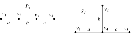
Figure 4. Path and star graphs with $4$ vertices

To derive further results about $W(\Gamma)$ by using Theorem 4.4, we need to understand the Wiener index of ${\overline{\Gamma}}_{i_{1},\dots,i_{v-4}}$ which is a tree with $4$ vertices. Thus, we consider Lemma 4.5 below.

Let $S_{n}$ and $P_{n}$ be star and path metrized graphs on $n$ vertices, respectively. Figure 4 illustrates $S_{4}$ and $P_{4}$.

Lemma 4.5.

Suppose metrized graph $\Gamma$ is a tree with $4$ vertices. Then $\Gamma$ is either $S_{4}$ or $P_{4}$. Moreover, $W(P_{4})=3(a+b+c)+b$ and $W(S_{4})=3(a+b+c)$, where edge lengths are as in Figure 4.

Proof.

A direct computation gives the result. ∎

Now, we can state our second main result for trees:

Theorem 4.6.

Let metrized graph $\Gamma$ be a tree with $v$ vertices. Suppose each edge length of $\Gamma$ is $1$. Then we have

$$\begin{split}W(\Gamma)&=(v-1)^{2}+\sum_{\begin{subarray}{c}\{e_{i_{1}},\,e_{i_{2}},\,\cdots,\,e_{i_{v-4}}\}\subset E(\Gamma)\\ {\overline{\Gamma}}_{i_{1},\dots,i_{v-4}}=P_{4}\end{subarray}}1,\\ &=(v-1)^{2}+\sum_{\begin{subarray}{c}\{e_{i_{1}},\,e_{i_{2}},\,e_{i_{3}}\}\subset E(\Gamma)\\ e_{i_{1}},e_{i_{2}},e_{i_{3}}\in P\\ \text{P is a path in $\Gamma$}\end{subarray}}1.\end{split}$$

The last summation is taken over all subsets $\{e_{i_{1}},\,e_{i_{2}},\,e_{i_{3}}\}$ of $E(\Gamma)$ such that the edges $e_{i_{1}}$, $e_{i_{2}}$ and $e_{i_{3}}$ are parts of a path in $\Gamma$.

Proof.

Applying Lemma 4.5 for this case, we obtain $W({\overline{\Gamma}}_{i_{1},\dots,i_{v-4}})=10$ if ${\overline{\Gamma}}_{i_{1},\dots,i_{v-4}}=P_{4}$, and $W({\overline{\Gamma}}_{i_{1},\dots,i_{v-4}})=9$ if ${\overline{\Gamma}}_{i_{1},\dots,i_{v-4}}=S_{4}$.

We note that

$$\begin{split}\frac{1}{(v-4)!}\sum_{\begin{subarray}{c}e_{i_{1}}\in\\ E(\Gamma)\end{subarray}}\sum_{\begin{subarray}{c}e_{i_{2}}\in\\ E({\overline{\Gamma}}_{i_{1}})\end{subarray}}\;\dots\sum_{\begin{subarray}{c}e_{i_{v-4}}\in\\ E({\overline{\Gamma}}_{i_{1},\dots,i_{v-5}})\end{subarray}}1=\frac{(v-1)(v-2)(v-3)}{6}.\end{split}$$

Then we use Theorem 4.4 with $\ell(\Gamma)=(v-1)$ to obtain

$$\begin{split}W(\Gamma)=(v-1)^{2}+\frac{1}{(v-4)!}\sum_{\begin{subarray}{c}e_{i_{1}},\,e_{i_{2}},\,\cdots,\,e_{i_{v-4}}\in E(\Gamma)\\ {\overline{\Gamma}}_{i_{1},\dots,i_{v-4}}=P_{4}\end{subarray}}1=(v-1)^{2}+\sum_{\begin{subarray}{c}\{e_{i_{1}},\,e_{i_{2}},\,\cdots,\,e_{i_{v-4}}\}\subset E(\Gamma)\\ {\overline{\Gamma}}_{i_{1},\dots,i_{v-4}}=P_{4}\end{subarray}}1.\end{split}$$

We have the second equality above, because the number of permutations of $v-4$ edges $e_{i_{1}},\,e_{i_{2}},\,\cdots,\,e_{i_{v-4}}$ is $(v-4)!$. This gives the first equality in the theorem.

The second equality in the theorem follows from the first one. ∎

Note that Theorem 4.6 in a sense gives information about how far a graph is away from being a star graph.

As a corollary to Theorem 4.6, we obtain the following well-known result:

Corollary 4.7.

For any metrized graph $\Gamma$ with $v$ vertices, we have

$$(v-1)^{2}=W(S_{v})\leq W(\Gamma)\leq W(P_{v})=\frac{v(v^{2}-1)}{6}.$$

Proof.

No path in $S_{v}$ can contain $3$ edges, so $W(S_{v})=(v-1)^{2}$ by using Theorem 4.6. Since this is the case with minimum value $0$ of the summation in the formula of Theorem 4.6, we obtain $W(S_{v})\leq W(\Gamma)$.

On the other hand, any $3$ edges in $P_{v}$ is part of a path in $P_{v}$, namely the path is $P_{v}$ itself. Thus, the summation in the formula of Theorem 4.6 is $\binom{v-1}{3}$, and so $W(P_{v})=(v-1)^{2}+\binom{v-1}{3}$ by Theorem 4.6. We note that $\binom{v-1}{3}$ is the maximum value of the summation, so $W(\Gamma)\leq W(P_{v})$. ∎

We recall the following result due to Doyle and Graver [12] to compare with Theorem 4.6:

Theorem 4.8.

[11, Theorem 9] Let metrized graph $\Gamma$ be a tree with $v$ vertices, and let $v_{1}$, $v_{2}$, $\dots$, $v_{\upsilon(p)}$ be the number vertices in the connected components of the graph obtained from $\Gamma$ by deleting the edges connected to a vertex $p$. Then

$$W(\Gamma)=\frac{v(v^{2}-1)}{6}-\sum_{\begin{subarray}{c}p\in V(\Gamma),\\ \upsilon(p)\geq 3\end{subarray}}\,\,\,\sum_{1\leq i<j<k\leq\upsilon(p)}v_{i}v_{j}v_{k}.$$

Note that Theorem 4.8 somewhat explains how far a graph is away from being a path graph.

Next, we restate Lemma 3.14 for trees. For an edge $e_{i}$ with end points $p_{i}$ and $q_{i}$, let $m_{i}$ be the number of vertices that are in the connected component of $\Gamma-e_{i}$ containing $p_{i}$, and let $k_{i}$ be the number of vertices that are in the connected component of $\Gamma-e_{i}$ containing $q_{i}$. Then we have $m_{i}+k_{i}=v$.

Theorem 4.9.

Let metrized graph $\Gamma$ be a tree with $v$ vertices. Suppose each edge length of $\Gamma$ is $1$. Then we have

$$\begin{split}W(\Gamma)=\sum_{e_{i}\in E(\Gamma)}m_{i}\cdot k_{i}.\end{split}$$

Proof.

Each edge $e_{i}$ is bridge, so $\frac{R_{i}}{L_{i}+R_{i}}\longrightarrow 0$. Moreover, ${\overline{\Gamma}}_{i_{1},\dots,i_{v-2}}$ is the edge that is not contracted, so we have $r_{{\overline{\Gamma}}_{i_{1},\dots,i_{v-2}}}(p^{\prime},q^{\prime})=1$. Therefore, Lemma 3.14 implies

$$W(\Gamma)=\frac{1}{(v-2)!}\sum_{\begin{subarray}{c}e_{i_{1}},\,e_{i_{2}},\,\cdots,\,e_{i_{v-2}}\in E(\Gamma)\end{subarray}}m\cdot k,$$

where $m$ and $k$ are as defined before. Considering the permutations of the contracted edges, we can rewrite this as

$$\begin{split}W(\Gamma)=\sum_{\begin{subarray}{c}\{e_{i_{1}},\,e_{i_{2}},\,\cdots,\,e_{i_{v-2}}\}\subset E(\Gamma)\end{subarray}}m\cdot k=\sum_{e_{i}\in E(\Gamma)}m\cdot k.\end{split}$$

Now, suppose ${\overline{\Gamma}}_{i_{1},\dots,i_{v-2}}=e_{i}$. Then the number of vertices contracted into $p_{i}$ is nothing but $m_{i}$, i.e., $m=m_{i}$. Similarly, the number of vertices contracted into $q^{\prime}$ is $k_{i}$. That is, $k=k_{i}$. This completes the proof. ∎

Note that Theorem 4.9 was known previously [11, page 218] and [14].

Example II: Let $\beta_{1}$ and $\beta_{2}$ be the metrized graphs with $s+t+2$ and $s+t+3$ vertices, respectively. These are illustrated in Figure 5. Suppose $s\geq 0$, $t\geq 0$ and each edge length in $\beta_{1}$ and $\beta_{2}$ is equal to 1. By applying Theorem 4.6, we obtain

$W(\beta_{1})=(s+t+1)^{2}+\binom{s}{1}\binom{t}{1}=(s+t+1)^{2}+s\cdot t$.

$W(\beta_{2})=(s+t+2)^{2}+\binom{s}{1}\binom{2}{1}\binom{t}{1}+\binom{s}{1}\binom{2}{2}\binom{t}{0}+\binom{s}{0}\binom{2}{2}\binom{t}{1}=(s+t+2)^{2}+2s\cdot t+s+t$.

Figure 5. Tree metrized graphs $\beta_{1}$ and $\beta_{2}$.

We note that these results agree with the results given in [11, page 234] (as $\beta_{1}=D(s+t+2,s,t)$ and $\beta_{2}=D(s+t+3,s,t)$, where $D(v,s,t)$ is the graph defined as in [11, page 234]).

Example III: In this example, we work with metrized graphs $\beta_{3}$ and $\beta_{4}$ illustrated in Figure 6. $\beta_{3}$ and $\beta_{4}$ have $s+t+k+4$ and $s+t+k+m+4$ vertices, respectively. Suppose $s\geq 0$, $t\geq 0$, $k\geq 0$, $m\geq 0$ and each edge length in these graphs is equal to 1. By applying Theorem 4.6, we obtain

$$\begin{split}W(\beta_{3})&=(s+t+k+3)^{2}+\binom{s}{1}\binom{2}{1}\binom{k}{1}+\binom{s}{1}\binom{2}{2}+\binom{2}{2}\binom{k}{1}+\binom{s}{1}\binom{2}{1}\binom{t}{1}\\ &\quad+\binom{s}{1}\binom{2}{2}+\binom{2}{2}\binom{t}{1}+\binom{k}{1}\binom{2}{1}\binom{t}{1}+\binom{k}{1}\binom{2}{2}+\binom{2}{2}\binom{t}{1}\\ &=(s+t+k+3)^{2}+2(sk+st+kt+s+t+k).\end{split}$$

Now, to compute $W(\beta_{4})$ we can use the computation used in obtaining $W(\beta_{3})$. Namely, when we compute the number of three edges that are part of a path in $\beta_{4}$, we can divide the edges in two groups: The ones having an end point in $\{u_{1},u_{2},\cdots,u_{m}\}$ and the ones with no end points in this set.

$$\begin{split}W(\beta_{4})&=(s+t+k+m+3)^{2}+2(sk+st+kt+s+t+k)+\binom{m}{1}\Big{[}\binom{s}{1}+\binom{k}{1}+\binom{t}{1}\Big{]}\\ &=(s+t+k+m+3)^{2}+2(sk+st+kt)+(m+2)(s+t+k).\end{split}$$

Figure 6. Tree metrized graphs $\beta_{3}$ and $\beta_{4}$.

Example IV: In this case, we work with metrized graph $\beta_{5}$ illustrated in Figure 7. $\beta_{5}$ has $v=s+t+k+m+n+5$ vertices. Suppose $s\geq 0$, $t\geq 0$, $k\geq 0$, $m\geq 0$, $n\geq 0$ and each edge length of $\beta_{5}$ is equal to 1. By applying Theorem 4.6 and using the computation of $W(\beta_{4})$, we obtain

$$W(\beta_{5})=(v-1)^{2}+2(sk+st+kt+mn+kn+sn)+(n+2)(s+k)+(m+2)(s+k+t+1)+n(t+5).$$

The details are left as an exercise to the reader.

Figure 7. Tree metrized graph $\beta_{5}$.

Example V: In this case, we work with metrized graph $\beta_{6}$ illustrated in Figure 7. $\beta_{6}$ has $v=s+t+k+m+n+h+6$ vertices. Suppose $s\geq 0$, $t\geq 0$, $k\geq 0$, $m\geq 0$, $n\geq 0$, $h\geq 0$ and each edge length of $\beta_{6}$ is equal to 1. By applying Theorem 4.6 and using the computation of $W(\beta_{5})$, we obtain

$$\begin{split}W(\beta_{6})&=(v-1)^{2}+2(sk+st+kt+mn+kn+sn)+(n+4)(s+k)+n(t+6)\\ &\quad+(m+2)(s+k+t+2)+h(3s+3k+2n+2m+t+6).\end{split}$$

The details are left as an exercise to the reader.

Figure 8. Tree metrized graph $\beta_{6}$.

Problem I: Show that the function $F:{\mathbb{N}}^{5}\longrightarrow{\mathbb{N}}$ given by $F(s,t,k,m,n)=(s+t+k+m+n+4)^{2}+2(sk+st+kt+mn+kn+sn)+(n+2)(s+k)+(m+2)(s+k+t+1)+n(t+5)$ takes every integer bigger than $557$, and that the only integers not assumed by $F$ are the following $89$ numbers:

$\{1,2,3,4,5,6,7,8,9,10,11,12,13,14,15,16,17,19,20,21,22,23,24,25,26,27,30,33,34,35,$ $36,37,38,39,41,43,45,47,49,51,52,53,55,56,60,61,69,73,75,77,78,79,81,83,85,87,89,91,$ $99,101,106,113,125,129,131,133,135,141,143,147,149,157,159,165,197,199,203,213,217,$ $219,281,285,293,301,325,357,501,509,557\}$.

We checked by a computer program that any integer not in the list above and less than $20000$ can be a value of $F$.

Problem II: Show that the function $G:{\mathbb{N}}^{6}\longrightarrow{\mathbb{N}}$ given by $G(s,t,k,m,n,h)=(s+t+k+m+n+h+5)^{2}+2(sk+st+kt+mn+kn+sn)+(n+4)(s+k)+(m+2)(s+k+t+2)+n(t+6)+h(3s+3k+2n+2m+t+6)$ takes every integer bigger than $301$, and that the only integers not assumed by $G$ are the following $104$ numbers:

$\{1,2,3,4,5,6,7,8,9,10,11,12,13,14,15,16,17,18,19,20,21,22,23,24,25,26,27,28,30,31,32,33,34,35,\quad$ $36,37,38,39,40,41,43,44,45,47,48,49,50,51,52,53,54,55,56,59,60,61,64,66,69,70,71,72,73,75,77,78,\quad$ $79,81,83,85,87,89,91,95,98,99,101,102,106,113,119,124,127,129,131,133,135,139,141,143,147,149,157,\qquad$ $159,165,197,199,203,213,217,219,279,293,301\}$.

Again, we tested by a computer program that any integer not in the list above and less than $20000$ can be a value of $G$.

The following theorem was conjectured in [16] and [13], and proved in both [20] and [19].

Theorem 4.10.

Except for exactly the following $49$ positive integers, every positive integer is the Wiener index of some tree.

$\{2,3,5,6,7,8,11,12,13,14,15,17,19,21,22,23,24,26,27,30,33,34,37,38,39,41,43,45,47,$ $51,53,55,60,61,69,73,77,78,83,85,87,89,91,99,101,106,113,147,159\}$.

Note that a positive solution to any of Problem I and Problem II above will be another proof of Theorem 4.10.

Acknowledgements: This work is supported by The Scientific and Technological Research Council of Turkey-TUBITAK (Project No: 110T686).

References

[1] M. Baker and X. Faber, Metrized graphs, Laplacian operators, and
electrical networks, Quantum graphs and their applications, 15–33,
Contemp. Math., 415, Amer. Math. Soc., Providence, RI, (2006).
[2] M. Baker and R. Rumely, Harmonic analysis on metrized graphs, Canadian
J. Math: 59, no. 2, 225–275, (2007).
[3] T. Chinburg and R. Rumely, The capacity pairing,
J. reine angew. Math. 434, 1–44, (1993).
[4] Z. Cinkir, The Tau Constant of Metrized Graphs,
Thesis at University of Georgia, (2007).
[5]Z. Cinkir, Generalized Foster’s identities, International Journal of Quantum Chemistry, Volume 111, Issue 10, (2011), 2228 -2233.
[6] Z. Cinkir, The tau constant and the discrete Laplacian matrix of a metrized graph, European Journal of Combinatorics, Volume 32, Issue 4, (2011), 639–655.
[7] Z. Cinkir, The tau constant of a metrized graph and its behavior under graph operations, The Electronic Journal of Combinatorics, Volume 18 (1), (2011), P81.
[8] Z. Cinkir, The tau constant and the edge connectivity of a metrized graph,
The Electronic Journal of Combinatorics, Volume 19, Issue 4, (2012), P46.
[9] Z. Cinkir, Deletion and contraction identities for the resistance values and the Kirchhoff index,
International Journal of Quantum Chemistry, Volume:111, Issue:15, (2011), 4030–4041.
[10] Z. Cinkir, Zhang’s Conjecture and the Effective Bogomolov Conjecture over function fields, Inventiones Mathematicae, Volume 183, Number 3, (2011) 517–562.
[11] A. A. Dobrynin, R. Entringer and I. Gutman, Wiener Index of Trees: Theory and Applications, Acta Applicandae Mathematicae, 66 (2001) 211 -249.
[12]J. K. Doyle and J. E. Graver, Mean distance in a graph, Discrete Math. 7, (1977), 147 -154.
[13] I. Gutman and Y. Yeh, The sum of all distances in bipartite graphs, Math. Slovaca 45, (1995), 327 -334.
[14] H. Wiener, Structural determination of paraffin boiling points, J. Amer. Chem. Soc. 69, (1947),
17 -20.
[15] D. J. Klein and M. Randić, Resistance
distance, Journal Mathematical Chemistry, 12, (1993), 81–95.
[16] M. Lepović and I. Gutman, A collective property of trees and chemical trees, J. Chem. Inf. Comput. Sci. 38, (1998), 823 -826.
[17] I. Lukovits, S. Nicolić and N. Trinajstić, Resistance distance in regular graphs, International Journal of Quantum Chemistry, Volume 71, Issue 3, (1999) 217 -225.
[18] R. Rumely, Capacity Theory on Algebraic Curves, Lecture Notes in
Mathematics 1378, Springer-Verlag, Berlin-Heidelberg-New York, (1989).
[19] S. G. Wagner, A Class of Trees and its Wiener Index, Acta. Appl. Math., 91, (2006) 119 132.
[20] H. Wang and G. Yu, All but 49 Numbers are Wiener Indices of Trees, Acta. Appl. Math. 92, (2006) 15 20.