On the Optimal General Convergence Rates for Quadratures Derived from Chebyshev Points

Abstract

In this paper, we study the optimal general convergence rates for quadratures derived from Chebyshev points. By building on the aliasing errors on integration of Chebyshev polynomials, together with the asymptotic formulae on the coefficients of Chebyshev expansions, new and optimal convergence rates for $n$-point Clenshaw-Curtis, Fejér’s first and second quadrature rules are established for Jacobi weights or Jacobi weights multiplied by $\ln((x+1)/2)$. The convergence orders are attainable for some functions of finite regularities. In addition, by using refined estimates on aliasing errors on integration of Chebyshev polynomials by Gauss-Legendre quadrature, an improved convergence rate for Gauss-Legendre is given too.

1 Introduction

The computation of integrals of the form of

(1) $$I[f]=\int_{-1}^{1}w(x)f(x)dx$$

is one of the oldest and most important issues in numerical analysis. Quadrature formulae are usually derived from polynomial interpolation by a finite sum

(2) $${\displaystyle I_{n}[f]=\sum_{j=1}^{n}w_{j}f(x_{j}),\quad x_{j}\in[-1,1]}.$$

Among all interpolation type quadrature rules with $n$ nodes, the Gauss-Christoffel formula, denoted by $I_{n}^{G}[f]$, has the highest accuracy of degree $2n-1$ (c.f. Davis and Rabinowitz [11], Gautschi [21]). Particularly, for Jacobi weight function $w(x)=(1-x)^{\alpha}(1+x)^{\beta}$ ($\alpha>-1$, $\beta>-1$), fast evaluation of the nodes and weights for the Gauss quadrature was given by Glaser, Liu and Rokhlin [22] with $O(n)$ operations, which has been recently extended by both Bogaert, Michiels and Fostier [2], and Hale and Townsend [23]. A Matlab file for computation of these nodes and weights can be found in Chebfun system [40].

It has been observed for a long time that, in the case $w(x)\equiv 1$, for most integrands, $n$-point Gauss and $n$-point Clenshaw-Curtis quadrature (denoted by $I_{n}^{C\texttt{-}C}[f]$) are about equally accurate (c.f. O’Hara and Smith [24], Evans [14] and Kythe and Schäferkotter [26]. For more details, see Trefethen [38]).

This observation was made precise by Trefethen [38, 39], by using new asymptotics on the coefficients of Chebyshev expansions for functions of finite regularity: Suppose $f(x)$ satisfies a Dini-Lipschitz condition on $[-1,1]$, then it has the following uniformly convergent Chebyshev series expansion (c.f. Cheney [7, p. 129])

(3) $$f(x)=\sum_{j=0}^{\infty}{{}^{\prime}}a_{j}T_{j}(x),$$

where the prime denotes summation whose first term is halved, $T_{j}(x)=\cos(j\cos^{-1}x)$ denotes the Chebyshev polynomial of degree $j$, and the Chebyshev coefficient $a_{j}$ is defined by

(4) $$a_{j}=\frac{2}{\pi}\int_{-1}^{1}\frac{f(x)T_{j}(x)}{\sqrt{1-x^{2}}}dx,\quad j=0,1,\ldots.$$

Trefethen in [38, 39] showed that for an integer $k\geq 1$, if $f(x)$ has an absolutely continuous $(k-1)$st derivative $f^{(k-1)}$ on $[-1,1]$ and a $k$th derivative $f^{(k)}$ of bounded variation $V_{k}={\rm Var}(f^{(k)})<\infty$, then for each $j\geq k+1$,

(5) $$|a_{j}|\leq{\displaystyle\frac{2V_{k}}{\pi j(j-1)\cdots(j-k)}},$$

and

(6) $${\frac{32V_{k}}{15k\pi(2n-1-k)^{k}}\geq}\left\{\begin{array}[]{ll}|I[f]-I_{n}^{G}[f]|&\mbox{for all $n\geq k/2+1$}\\ |I[f]-I_{n}^{C\texttt{-}C}[f]|&\mbox{for all sufficiently large $n$}\end{array}.\right.$$

Chebyshev expansions are very useful tools for numerical analysis. Their convergence is guaranteed under rather general conditions and they often converge fast compared with other polynomial expansions (c.f. Fox and Parker [18], Hesthaven et al. [25], Petras [30] and Xiang [44]). For example, it has been shown that the coefficient $a_{j}$ of the Chebyshev expansion of $f$ decays a factor of $\sqrt{j}$ faster than the corresponding coefficient of the Legendre expansion, which is mentioned in [18, p. 17] and Boyd [3, p. 52], and made precise in [44] and Wang and Xiang [42]. Additionally, the quadrature errors of the Gauss and Clenshaw-Curtis can be represented by using the Chebyshev expansion, respectively, if $\sum_{j=1}^{\infty}a_{j}$ is absolutely convergent, as

(7)      $${\displaystyle E_{n}^{G}[f]=I[f]-I_{n}^{G}[f]=\sum_{j=2n}^{\infty}a_{j}E_{n}^{G}[T_{j}],\,E_{n}^{C\texttt{-}C}[f]=I[f]-I_{n}^{C\texttt{-}C}[f]=\sum_{j=n}^{\infty}a_{j}E_{n}^{C\texttt{-}C}[T_{j}]}$$.

A new convergence rate improved one further power of $n$ for $n$-point Gauss and Clenshaw-Curtis quadrature is given in Xiang and Bornemann [45] for $f\in X^{s}$ ($s>0$), based on the work of Curtis and Rabinowitz [9] and Riess and Johnson [32] from the early 1970s, and a refined estimate for Gauss quadrature applied to Chebyshev polynomials due to Petras in 1995 [30]. Here, we say $f\in X^{s}$ if the Chebyshev coefficient $a_{j}$ satisfies that $a_{j}=O(j^{-s-1})$ [45]. Moreover, from [38, 39], we see that if $f(x)$ has an absolutely continuous $(k-1)$st derivative $f^{(k-1)}$ on $[-1,1]$ (if $k\geq 1$) and $V_{k}<\infty$ then $f\in X^{k}$.

In this paper, along the way to [9, 32, 38, 39, 45], by using refined estimates on the aliasing errors about the integration of Chebyshev polynomials by Gauss quadrature, in Section 2, we will improve the convergence rate for $n$-point Gauss-Legendre quadrature for $f\in X^{s}$ as

$$E_{n}^{G}[f]=\left\{\begin{array}[]{ll}O(n^{-2s}),&0<s<1\\ O(n^{-2}\ln n),&s=1\\ O(n^{-s-1}),&s>1\end{array}.\right.$$

In Section 3, we will present optimal general convergence rates for generalized $n$-point Clenshaw-Curtis quadrature, Fejér’s first and second rules for $f\in X^{s}$ for the following weights:

• for $w(x)=(1-x)^{\alpha}(1+x)^{\beta}$:

  $$E_{n}[f]=\left\{\begin{array}[]{ll}O(n^{-s-1})&\mbox{if $\min(\alpha,\beta)\geq-\frac{1}{2}$}\\ O(n^{-s-2-2\min(\alpha,\beta)})&\mbox{if $-1<\min(\alpha,\beta)<-\frac{1}{2}$}\end{array},\right.$$

• for $w(x)=\ln((x+1)/2)(1-x)^{\alpha}(1+x)^{\beta}$:

  $$E_{n}[f]=\left\{\begin{array}[]{ll}O(n^{-s-1})&\mbox{if $\beta>-\frac{1}{2}$}\\ O(n^{-s-2-2\beta}\ln n)&\mbox{if $-1<\beta\leq-\frac{1}{2}$}\end{array}.\right.$$

Without ambiguity, here $E_{n}[f]$ denotes the quadrature error of the $n$-point Clenshaw-Curtis quadrature, Fejér’s first and second rules for function $f\in X^{s}$, respectively. It is worth noting that these convergence orders are attainable for some functions of finite regularities. Final remarks on comparison with the convergence rate of Gauss quadrature is included in Section 4.

2 An improved error bound on the Gauss quadrature for $w(x)\equiv 1$

Let $x_{k}$ be the zeros of the Legendre polynomial of degree $n$, ordered by $-1<x_{1}<x_{2}<\cdots<x_{n}<1$, and $w_{k}$ the corresponding weights in the $n$-point Gauss quadrature ($k=1,2,\ldots,n$).

Xiang and Bornemann [45] showed for $f\in X^{s}$ that

(8) $$E_{n}^{G}[f]=\left\{\begin{array}[]{ll}O(n^{-3s/2}),&0<s<2\\ O(n^{-s-1}),&s\geq 2\end{array},\right.\mbox{while $E_{n}^{C\texttt{-}C}[f]=O(n^{-s-1})$ for $s>0$},$$

by applying the asymptotic formulae for $x_{k}=-\cos\theta_{k}$ and $w_{k}$ for $1\leq k\leq\lfloor(n+1)/2\rfloor$

(9) $$\,\,\,\,\,\,\theta_{k} = \phi_{k}+\frac{1}{2(2n+1)^{2}}\cot\phi_{k}+\delta_{k},\quad\phi_{k}=\frac{4k-1}{4n+2}\pi\quad\mbox{(c.f. Gatteschi \cite[cite]{[\@@bibref{}{Gatteschi87}{}{}]})},$$

(10) $$\,\,\,\,\,\,w_{k} = \frac{2\pi}{2n+1}\sin\phi_{k}\left(1-\frac{1}{2(2n+1)^{2}}\right)(1+\epsilon_{k})\quad\mbox{(c.f. F\"{o}rster and Petras \cite[cite]{[\@@bibref{}{ForsterPetras93}{}{}]})},$$

where

(11) $$\quad 0\leq-\delta_{k}\leq\frac{11\cos\phi_{k}}{8(2n+1)^{4}\sin^{3}\phi_{k}},\quad-\frac{\cos^{2}\phi_{k}}{(2n+1)^{4}\sin^{4}\phi_{k}}\leq\epsilon_{k}\leq\frac{8}{(2n+1)^{4}\sin^{4}\phi_{k}},$$

together with the error estimate given by Petras [30] for $m=j(4n+2)+2r$

$$|E_{n}^{G}[T_{m}]|=\left\{\begin{array}[]{ll}\frac{2+O(mr/n^{2})}{|4r^{2}-1|}+O(m^{4}/n^{6})+O(m^{2}\log n/n^{2}),&-n<r<n\\ \frac{\pi}{2}+O(m/n^{2})+O(m^{4}/n^{6})+O(m\log n/n^{2}),&r=\pm n\end{array}.\right.$$

By using the following refined estimates, we can get an improved convergence rate on the Gauss quadrature.

Lemma 1.

The aliasing and aliasing errors about the integration of Chebyshev polynomials by the $n$-point Gauss quadrature satisfy that for $j\geq 1$,

(14) $$\quad\quad I_{n}^{G}[T_{m}] = \left\{\begin{array}[]{ll}(-1)^{j}\frac{2}{1-4r^{2}}+O(m/n^{2}),&\ m=j(4n+2)+2r,\quad-n<r<n\\ \pm(-1)^{j}\frac{\pi}{2}+O(m/n^{2}),&\ m=(2j-1)(2n+1)\pm 1\end{array},\right.$$

(17) $$\quad\quad\quad|E_{n}^{G}[T_{m}]| = \left\{\begin{array}[]{ll}\frac{2}{|4r^{2}-1|}+O(m/n^{2}),&\ m=j(4n+2)+2r,\quad-n<r<n\\ \frac{\pi}{2}+O(m/n^{2}),&\ m=(2j-1)(2n+1)\pm 1\end{array}.\right.$$

Proof.

For the case $m=j(4n+2)+2r$ with $-n<r<n$ and $j\geq 1$: From (2.1), we have

$$m\theta_{k}=j(4n+2)\theta_{k}+2r\theta_{k}=j(4k-1)\pi+h_{k}+2r\theta_{k},$$

where

(18) $$h_{k}=\frac{j(4n+2)}{2(2n+1)^{2}}\cot\phi_{k}+j(4n+2)\delta_{k},$$

and get

$$\begin{array}[]{lll}\cos m\theta_{k}&=&\cos(j(4k-1)\pi+h_{k}+2r\theta_{k})\\ &=&(-1)^{j}\cos h_{k}\cos 2r\theta_{k}-(-1)^{j}\sin h_{k}\sin 2r\theta_{k}\\ &=&(-1)^{j}(1+\cos h_{k}-1)\cos 2r\theta_{k}-(-1)^{j}\sin h_{k}\sin 2r\theta_{k}\\ &=&(-1)^{j}\cos 2r\theta_{k}-2(-1)^{j}\sin\frac{h_{k}}{2}\sin\left(\frac{h_{k}}{2}+2r\theta_{k}\right),\end{array}$$

which yields

(19)   $${\displaystyle I_{n}^{G}[T_{m}]=\sum_{k=1}^{n}w_{k}\cos m\theta_{k}=(-1)^{j}I[T_{|2r|}]-2(-1)^{j}\sum_{k=1}^{n}w_{k}\sin\frac{h_{k}}{2}\sin\left(\frac{h_{k}}{2}+2r\theta_{k}\right).}$$

Furthermore, note that

(20) $${\small\begin{array}[]{lll}{\displaystyle\Big{|}\sum_{k=1}^{n}w_{k}\sin\frac{h_{k}}{2}\sin\left(\frac{h_{k}}{2}+2r\theta_{k}\right)\Big{|}}&\leq&{\displaystyle\sum_{k=1}^{\lfloor(n+1)/2\rfloor}w_{k}|h_{k}|}\\ &\leq&{\displaystyle\sum_{k=1}^{\lfloor(n+1)/2\rfloor}w_{k}\left(\frac{j(4n+2)}{2(2n+1)^{2}}\cot\phi_{k}+j(4n+2)|\delta_{k}|\right).}\end{array}}$$

From the estimate on $\delta_{k}$ (2.3) and using $\frac{2}{\pi}\phi_{k}\leq\sin\phi_{k}\leq\phi_{k}$ for $0<\phi_{k}\leq\frac{\pi}{2}$, we obtain

$$\delta_{k}=O(n^{-1}k^{-3}),$$

and applying an $O(n^{-1})$ bound on the weights from (2.2) or Szegö [37], we obtain

(21) $$\sum_{k=1}^{\lfloor(n+1)/2\rfloor}w_{k}j(4n+2)|\delta_{k}|=O(m/n^{2})\sum_{k=1}^{\lfloor(n+1)/2\rfloor}\frac{1}{k^{3}}=O(m/n^{2}).$$

Moreover, by (2.2) and (2.3), it is easy to derive that

$$w_{k}=\frac{2\pi}{2n+1}\sin\phi_{k}+O(n^{-2}k^{-1}),$$

which, together with the estimate $\cot\phi_{k}\leq\frac{1}{\sin\phi_{k}}\leq\frac{1}{\frac{2}{\pi}\phi_{k}}=\frac{(2n+1)}{4k-1}$, induces

(22) $$\begin{array}[]{lll}&&{\displaystyle\sum_{k=1}^{\lfloor(n+1)/2\rfloor}w_{k}\frac{j(4n+2)\pi}{2(2n+1)^{2}}\cot\phi_{k}}\\ &=&{\displaystyle\sum_{k=1}^{\lfloor(n+1)/2\rfloor}\frac{j(4n+2)\pi^{2}}{(2n+1)^{3}}\cos\phi_{k}+\sum_{k=1}^{\lfloor(n+1)/2\rfloor}\frac{j(4n+2)O(n^{-2}k^{-1})}{2(2n+1)^{2}}\cot\phi_{k}}\\ &=&{\displaystyle O(m/n^{2})\int_{0}^{\pi/2}\cos tdt+O(m/n^{3})\sum_{k=1}^{\lfloor(n+1)/2\rfloor}\frac{1}{k^{2}}}\\ &=&{\displaystyle O(m/n^{2})}.\end{array}$$

Combining (2.9)-(2.11) derives ${\displaystyle\sum_{k=1}^{n}w_{k}\sin\frac{h_{k}}{2}\sin\left(\frac{h_{k}}{2}+2r\theta_{k}\right)=O(m/n^{2})}$. Consequently, by (2.8) we get (2.5), and then using $I[T_{2\ell}]=\frac{2}{1-4\ell^{2}}$ for $\ell\geq 0$ we get (2.6), in the case $m=j(4n+2)+2r$ with $-n<r<n$ and $j\geq 1$.

For the case $m=(2j-1)(2n+1)\pm 1$: $\cos m\theta_{k}$ can be written by (2.1) as

$$\begin{array}[]{lll}\cos m\theta_{k}&=&\cos((2j-1)(2n+1)\theta_{k}\pm\theta_{k})\\ &=&\cos\left(\frac{(2j-1)(4k-1)}{2}\pi+\widetilde{h}_{k}\pm\theta_{k}\right)\\ &=&(-1)^{j+1}\sin(\widetilde{h}_{k}\pm\theta_{k})\\ &=&(-1)^{j+1}\sin\widetilde{h}_{k}\cos\theta_{k}\pm(-1)^{j+1}[1+(\cos(\widetilde{h}_{k})-1)]\sin\theta_{k}\\ &=&\pm(-1)^{j+1}\sin\theta_{k}+2(-1)^{j+1}\sin\frac{\widetilde{h}_{k}}{2}\cos\left(\frac{\widetilde{h}_{k}}{2}\pm\theta_{k}\right),\end{array}$$

where

$$\widetilde{h}_{k}=\frac{(2j-1)(2n+1)}{2(2n+1)^{2}}\cot\phi_{k}+(2j-1)(2n+1)\delta_{k}.$$

By the same arguments as those for the estimate of $\sum_{k=1}^{n}w_{k}|h_{k}|$, similarly, we have $\sum_{k=1}^{n}w_{k}|\widetilde{h}_{k}|=O(m/n^{2})$ and then

(23) $$\begin{array}[]{lll}I_{n}^{G}[T_{m}]&=&{\displaystyle\pm(-1)^{j+1}\sum_{k=1}^{n}w_{k}\sin\theta_{k}+2(-1)^{j+1}\sum_{k=1}^{n}w_{k}\sin\frac{\widetilde{h}_{k}}{2}\cos\left(\frac{\widetilde{h}_{k}}{2}\pm\theta_{k}\right)}\\ &=&{\displaystyle\pm(-1)^{j+1}\sum_{k=1}^{n}w_{k}\sin(-\cos^{-1}x_{k})+O(m/n^{2})}\\ &=&\pm(-1)^{j}I_{n}^{G}[\sqrt{1-x^{2}}]+O(m/n^{2}).\end{array}$$

Furthermore, from Förster and Petras [16], we find that

$$|I_{n}^{G}[\sqrt{1-x^{2}}]-I[\sqrt{1-x^{2}}]|=|2(I[g(x)]-I_{n}^{G}[g(x)])|\leq 2\sin^{2}\frac{2\pi}{(2n+1)^{2}}$$

by setting $g(x)=-\frac{1}{2}\sqrt{1-x^{2}}$ and applying the fact that $g$ is convex on $[-1,1]$ with $g(-1)-2g(0)+g(1)=1$, which, together with $I[\sqrt{1-x^{2}}]=\frac{\pi}{2}$, $I[T_{2\ell}]=\frac{2}{1-4\ell^{2}}$ for $\ell\geq 0$ and (2.12), derives the desired results in the case $m=(2j-1)(2n+1)\pm 1$. ∎

Theorem 2.

If $f\in X^{s}$, the error of the $n$-point Gauss quadrature has the rate

(24) $$E_{n}^{G}(f)=\left\{\begin{array}[]{ll}O(n^{-2s}),&0<s<1\\ O(n^{-2}\ln n),&s=1\\ O(n^{-s-1}),&s>1\end{array}.\right.$$

Proof.

With $f\in X^{s}$, that is, $a_{m}=O(m^{-s-1})$ for some $s>0$, we see that

$${\displaystyle E^{G}_{n}[f]=\sum_{m=2n}^{\infty}a_{m}E^{G}_{n}[T_{m}]}$$

is uniformly and absolutely convergent since $a_{m}=O(m^{-s-1})$ and $|E_{n}^{G}[T_{m}]|\leq\frac{32}{15}$ for $m\geq 4$ (c.f. Brass and Petras [5]). Then $E_{n}^{G}[f]$ can be estimated, by the asymptotics on $a_{m}$, estimates (2.6) on $|E_{n}^{G}[T_{m}]|$ and using $E_{n}^{G}[T_{2k+1}]=0$ for $k=0,1,\ldots$, as

$$\begin{array}[]{lll}\Big{|}E_{n}^{G}(f)\Big{|}&=&{\displaystyle\Big{|}\sum_{j=1}^{n}\sum_{|r|<n}a_{j(4n+2)+2r}E_{n}^{G}(T_{j(4n+2)+2r})}\\ &&{\displaystyle+\sum_{j=1}^{n}a_{(2j-1)(2n+1)\pm 1}E_{n}^{G}(T_{(2j-1)(2n+1)\pm 1})+\sum_{m=4n(n+1)}^{\infty}a_{m}E_{n}^{G}[T_{m}]}\Big{|}\\ &=&O\left({\displaystyle\sum_{j=1}^{n}\sum_{|r|<n}\frac{2/|4r^{2}-1|}{(j(4n+2)+2r)^{1+s}}+\sum_{j=1}^{n}\frac{\pi}{((2j-1)(2n+1)\pm 1)^{1+s}}}\right)\\ &&{\displaystyle+O\left(\frac{1}{n^{2}}\right)\sum_{m=2n}^{4n(n+1)-1}\frac{1}{m^{s}}+O\left(\sum_{m=4n(n+1)}^{\infty}\frac{|E_{n}^{G}[T_{m}]|}{m^{1+s}}\right)}\\ &=&{\displaystyle O\left(\frac{1}{n^{1+s}}\right)+O\left(\frac{1}{n^{2}}\right)\sum_{m=2n}^{4n(n+1)-1}\frac{1}{m^{s}}+O\left(\sum_{m=4n(n+1)}^{\infty}\frac{1}{m^{1+s}}\right)}\\ &=&{\displaystyle O\left(\frac{1}{n^{1+s}}\right)+O\left(\frac{1}{n^{2}}\int_{2n}^{4n(n+1)-1}x^{-s}dx\right)+O\left(\frac{1}{n^{2s}}\right)},\end{array}$$

which leads to the desired result based up $0<s<1$, $s=1$ and $s>1$, respectively. ∎

Remark 1. The convergence rate (2.13) is optimal for $s>1$, which is verified similarly with $f_{s}(x)=|x-0.3|^{s}\in X^{s}$ used in [45] (see the right two columns in Figures 2.1-2.2, respectively). While for $f\in X^{s}$ with $0<s\leq 1$, the convergence rate (2.13) is better than that in [45]. However, the numerical examples in [45] show that the $n$-point Gauss quadrature also enjoys the same convergence rate $O(n^{-s-1})$ (see the left column in Figures 2.1-2.2, respectively).

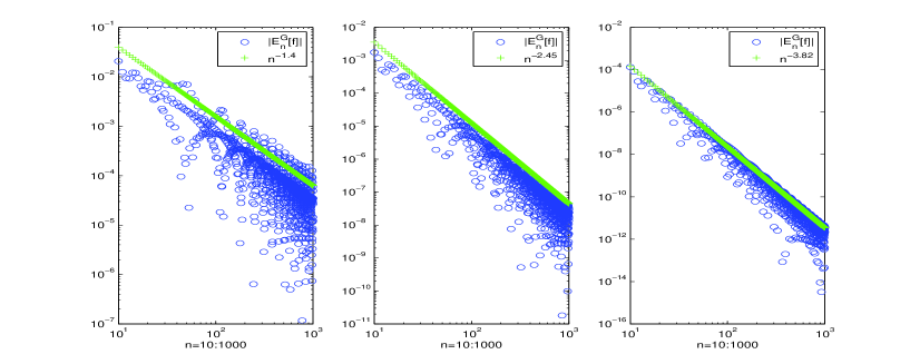
Fig. 1: The absolute errors for $n$-point Gauss for $f(x)=|x-0.3|^{s}$ ($f\in X^{s}$) with $s=0.4,1.45,2.82$, respectively: $n=10:1000$.

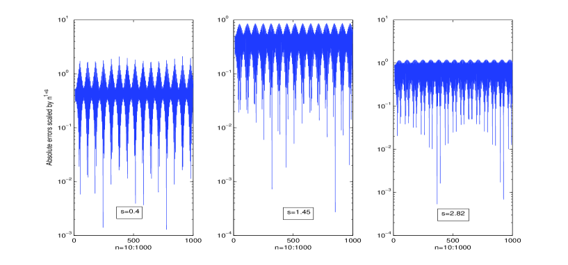
Fig. 2: The absolute errors scaled by $n^{1+s}$ for $n$-point Gauss for $f(x)=|x-0.3|^{s}$ ($f\in X^{s}$) with $s=0.4,1.45,2.82$, respectively: $n=10:1000$.

Remark 2. These techniques are difficult to be extended to study Gauss-Christoffel quadrature for general Jacobi weight functions. However, following the ideas of Riess and Johnson [32], Trefethen [38, 39] and Xiang and Bornemann [45], the optimal general convergence rates for generalized $n$-point Clenshaw-Curtis quadrature, Fejér’s first and second rules are not difficult to be obtained.

3 Clenshaw-Curtis and Fejér quadrature involving Jacobi weights

Fejér [15] in 1933 suggested using the zeros of a Chebyshev polynomial of first or second kind as interpolation points for quadrature rules of the form (1.2). Here we consider the generalized Fejér and Clenshaw-Curtis quadrature. Fejér’s first rule uses the zeros of the Chebyshev polynomial $T_{n}(x)$ of the first kind (also called classic Chebyshev points [11, 34, 35])

$$I_{n}^{F_{1}}[f]=\int_{-1}^{1}w(x)q_{n-1}^{1}(x)dx=\sum_{j=0}^{n-1}b_{j}^{1}\int_{-1}^{1}w(x)T_{j}(x)dx,$$

where $q_{n-1}^{1}$ is the interpolation polynomial defined by

$$\quad q_{n-1}^{1}(x)=\sum_{j=0}^{n-1}b_{j}^{1}T_{j}(x),\quad q_{n-1}^{1}(y_{j})=f(y_{j}),\,\,\,y_{j}=\cos\left(\frac{(2j-1)\pi}{2n}\right),\,j=1,2,\ldots,n,$$

while Fejér’s second rule uses the zeros of the Chebyshev polynomial $U_{n}(x)$ of the second kind (also called Filippi points [11])

$$I_{n}^{F_{2}}[f]=\int_{-1}^{1}w(x)q_{n-1}^{2}(x)dx=\sum_{j=0}^{n-1}b_{j}^{2}\int_{-1}^{1}w(x)T_{j}(x)dx,$$

where $q_{n-1}^{2}(x)$ is defined by

$$\quad q_{n-1}^{2}(x)=\sum_{j=0}^{n-1}b_{j}^{2}T_{j}(x),\quad q_{n-1}^{2}(x_{j})=f(x_{j}),\quad x_{j}=\cos\left(\frac{j\pi}{n+1}\right),\quad j=1,2,\ldots,n.$$

Clenshaw-Curtis quadrature (c.f. Clenshaw-Curtis [8]) is to use the above Chebyshev points with $n-1$ instead of $n+1$ including the endpoints $-1$ and $1$:

$$I_{n}^{C\texttt{-}C}[f]=\int_{-1}^{1}w(x)q_{n-1}^{3}(x)dx=\sum_{j=0}^{n-1}b_{j}^{3}\int_{-1}^{1}w(x)T_{j}(x)dx,$$

where $q_{n-1}^{3}$ is defined by

$$\quad q_{n-1}^{3}(x)=\sum_{j=0}^{n-1}b_{j}^{3}T_{j}(x),\quad q_{n-1}^{3}(\overline{x}_{j})=f(\overline{x}_{j}),\quad\overline{x}_{j}=\cos\left(\frac{j\pi}{n-1}\right),\,\,j=0,1,\ldots,n-1.$$

The coefficients $b_{j}^{i}$ ($i=1,2,3$) in the above three interpolation polynomials can be fast computed by FFT (c.f. Dahlquist and Björck [10], Trefethen [38], Waldvogel [41] and Xiang et al. [43, 46]).

In addition, the modified moments $\int_{-1}^{1}w(x)T_{j}(x)dx$ can be efficiently evaluated by recurrence formulae for Jacobi weights or Jacobi weights multiplied by $\ln((x+1)/2)$ (c.f. Piessens and Branders [31]).

• $w(x)=(1-x)^{\alpha}(1+x)^{\beta}$: The recurrence formulae for the evaluation of the modified moments

  (25) $$M_{k}(\alpha,\beta)=\int_{-1}^{1}w(x)T_{k}(x)dx,\quad w(x)=(1-x)^{\alpha}(1+x)^{\beta}$$

  are

  (26)      $$(\beta+\alpha+k+2)M_{k+1}(\alpha,\beta)+2(\alpha-\beta)M_{k}(\alpha,\beta)+(\beta+\alpha-k+2)M_{k-1}(\alpha,\beta)=0$$

  with

  $$M_{0}(\alpha,\beta)=2^{\beta+\alpha+1}\frac{\Gamma(\alpha+1)\Gamma(\beta+1)}{\Gamma(\beta+\alpha+2)},\quad M_{1}(\alpha,\beta)=2^{\beta+\alpha+1}\frac{\Gamma(\alpha+1)\Gamma(\beta+1)}{\Gamma(\beta+\alpha+2)}\frac{\beta-\alpha}{\beta+\alpha+2}.$$

  Furthermore, the asymptotic expression is given by using the asymptotic theory of Fourier coefficients (c.f. Lighthill [27]) as

  $${\small\begin{array}[]{lll}&&M_{k}(\alpha,\beta)\\ &\sim&-2^{\beta-\alpha}\cos(\pi\alpha)\Gamma(2\alpha+2)[k^{-2-2\alpha}+O(k^{-2\alpha-4})]\\ &&+(-1)^{k+1}2^{\alpha-\beta}\cos(\pi\beta)\Gamma(2\alpha+2)[k^{-2-2\beta}+O(k^{-2\beta-4})],\quad k\rightarrow\infty.\end{array}}$$

  The forward recursion is perfectly numerically stable, except in two cases:

  (27) $$\alpha>\beta\quad\mbox{and\quad}\beta = -\frac{1}{2},\frac{1}{2},\frac{3}{2},\ldots,$$

  (28) $$\beta>\alpha\quad\mbox{and\quad}\alpha = -\frac{1}{2},\frac{1}{2},\frac{3}{2},\ldots.$$

• $w(x)=\ln((x+1)/2)(1-x)^{\alpha}(1+x)^{\beta}$: For

  (29) $$G_{k}(\alpha,\beta)=\int_{-1}^{1}\ln((x+1)/2)(1-x)^{\alpha}(1+x)^{\beta}T_{k}(x)dx,$$

  the recurrence formulae are

  (30) $${\small\begin{array}[]{lll}&&(\beta+\alpha+k+2)G_{k+1}(\alpha,\beta)+2(\alpha-\beta)G_{k}(\alpha,\beta)\\ &&\quad+(\beta+\alpha-k+2)G_{k-1}(\alpha,\beta)=2M_{k}(\alpha,\beta)-M_{k-1}(\alpha,\beta)-M_{k+1}(\alpha,\beta)\end{array}}$$

  with

  $$G_{0}(\alpha,\beta)=-2^{\beta+\alpha+1}\Phi(\alpha,\beta+1),\quad G_{1}(\alpha,\beta)=-2^{\beta+\alpha+1}[2\Phi(\alpha,\beta+2)-\Phi(\alpha,\beta+1)],$$

  where

  $$\Phi(\alpha,\beta)=B(\alpha+1,\beta)[\Psi(\alpha+\beta+1)-\Psi(\beta)],$$

  $B(x,y)$ is the Beta function and $\Psi(x)$ is the Psi function (c.f. Abramowitz and Stegun [1]). Additionally, the asymptotic expression is given by using the asymptotic theory of Fourier coefficients as

  $$\begin{array}[]{lll}&&G_{k}(\alpha,\beta)\\ &\sim&(-1)^{k+1}2^{\alpha-\beta+1}\cos(\pi\beta)\Gamma(2\beta+2)k^{-2-2\beta}[-\ln 2k+\Psi(2\beta+2)\\ &&-\frac{\pi}{2}\tan\pi\beta]-2^{\beta-\alpha-2}\cos(\pi\alpha)\Gamma(2\alpha+4)k^{-4-2\alpha},\quad k\rightarrow\infty.\end{array}$$

  The forward recursion is also perfectly numerically stable the same as that for (3.2). For more details, see Piessens and Branders [31].

The convergence for the generalized $n$-point Clenshaw-Curtis quadrature, Fejér’s first and second rules, for

$$I[f]=\int_{-1}^{1}k(x)f(x)dx$$

with $\int_{-1}^{1}|k(x)|^{p}dx<\infty$ for some $p>1$, has been extensively studied in Elliott and Paget [13], Sloan [33] and Sloan and Smith [34, 35], etc. Taking into the Banach-Steinhaus (or uniform boundedness) theorem, using the convergence of Fourier series and Marcinkiewicz’s inequality [29, Vol. 2, pp. 28-30], Sloan [33] and Sloan and Smith [34] showed that the sums of the absolute values of the weights in (1.2) for the $n$-point Clenshaw-Curtis and Fejér’s first rule are uniformly bounded, i.e.

(31) $$\lim_{n\rightarrow\infty}\sum_{j=1}^{n}|w_{j}|=\int_{-1}^{1}|k(x)|dx,$$

and extended to the point set $\left\{\cos\left(\frac{2(i-1)\pi}{2n-1}\right)\right\}_{i=1}^{n}$. Identity (3.7) is also satisfied by $I_{n}^{F_{2}}[f]$.

Lemma 3.

Suppose $I[f]=\int_{-1}^{1}k(x)f(x)dx$ with $\int_{-1}^{1}|k(x)|^{p}dx<\infty$ for some $p>1$, then the weights of $I_{n}^{F_{2}}[f]$ satisfy (3.7).

Proof.

Since the weights of $I_{n}^{F_{2}}[f]$ can be represented as

$$w_{i}=\frac{2\sin\theta_{i}}{n+1}\sum_{j=0}^{n-1}\sin((j+1)\theta_{i})\overline{b}_{j+1},\quad\overline{b}_{i}=\int_{-1}^{1}k(x)U_{i-1}(x)dx,\quad i=1,2,\ldots,n$$

(c.f. [36]). Define an odd, $2\pi$-periodic function $K$ by

$$K(\theta)=\left\{\begin{array}[]{ll}\frac{\pi}{2}k(\cos\theta),&0\leq\theta\leq\pi\\ -\frac{\pi}{2}k(\cos\theta),&-\pi\leq\theta<0\end{array}.\right.$$

Then $\overline{b}_{j}$ has the form of

$$\overline{b}_{j}=\frac{2}{\pi}\int_{0}^{\pi}K(\theta)\sin(j\theta)d\theta,\quad j=1,2,\ldots,n,$$

which is the $j$th Fourier sine coefficient of $K$. In particular, the weight $w_{i}$ can be written as

$$w_{i}=\frac{2\sin\theta_{i}}{n+1}\sum_{j=1}^{n}\sin(j\theta_{i})\overline{b}_{j}=\frac{2}{n+1}S_{n}(\theta_{i})\sin\theta_{i},\quad i=1,2,\ldots,n,$$

where $S_{n}(\theta)$ is the $n$th partial sum of the Fourier series for the function $K(\theta)$. Therefore, the sum of the absolute values of the weights becomes

$$\sum_{j=1}^{n}|w_{i}|=\frac{2}{n+1}\sum_{j=1}^{n}|S_{n}(\theta_{i})|\sin\theta_{i},$$

which, by directly following a similar proof to [34], establishes

$$\lim_{n\rightarrow\infty}\sum_{j=1}^{n}|w_{j}|=\frac{2}{\pi}\int_{0}^{\pi}|K(\theta)|\sin\theta d\theta=\int_{-1}^{1}|k(x)|dx.$$

∎

Theorem 4.

Suppose $I[f]=\int_{-1}^{1}k(x)f(x)dx$ with $\int_{-1}^{1}|k(x)|^{p}dx<\infty$ for some $p>1$, then $\lim_{n\rightarrow\infty}I_{n}^{F_{2}}[f]=I[f]$ for all continuous functions in $[-1,1]$.

Proof.

By Lemma 3.1, it directly follows from [34]. ∎

Based upon these uniform boundedness, we see that for $f\in X^{s}$ with $s>0$,

$$|E_{n}[f]|=|I[f]-I_{n}[f]|=\Big{|}\sum_{j=n}^{\infty}a_{j}E_{n}[T_{j}]\Big{|}\leq\sum_{j=n}^{\infty}|a_{j}||E_{n}[T_{j}]|$$

since $a_{j}=O(j^{-1-s})$ and $E_{n}[T_{j}]$ are uniformly bounded for $j\geq 0$, where $E_{n}$ denotes the error of the above these three $n$-point quadrature rules corresponding to the two Jacobi weight functions. Furthermore, any rearrangement of the infinite sum $\sum_{j=n}^{\infty}|a_{j}||E_{n}[T_{j}]|$ converges to the same sum.

In the following, we will consider aliasing errors on the integration of the Chebyshev polynomials by these three quadrature rules, and derive the optimal general rate of convergence.

The computation of the aliasings by the Clenshaw-Curtis, Fejér first and second rules is much simple, which can be exactly computed from Fox and Parker [18, p. 67]

(32) $$T_{2pn\pm j}(y_{i})=\cos\left((2pn\pm j)\frac{(2i+1)\pi}{2n}\right)=(-1)^{p}\cos\left(\frac{j(2i+1)\pi}{2n}\right)=(-1)^{p}T_{j}(y_{i})$$

(33) $$T_{2p(n+1)\pm j}(x_{\ell})=\cos\left((2p(n+1)\pm j)\frac{\ell\pi}{n+1}\right)=\cos\left(\frac{j\ell\pi}{n+1}\right)=T_{j}(x_{\ell})$$

for $i,j=0,1,\ldots,n-1$, $\ell=1,2,\ldots,n$ and $p=1,2,\ldots$ as

(34) $$I_{n}^{F_{1}}[T_{2pn\pm j}]=(-1)^{p}I[T_{j}],\quad I_{n}^{F_{1}}[T_{2p(n-1)}]=0,\quad I_{n}^{F_{2}}[T_{2p(n+1)\pm j}]=I[T_{j}],$$

(35) $$\quad I_{n}^{F_{2}}[T_{(2p+1)(n+1)\pm 1}]=I_{n}^{F_{2}}[T_{n}],\quad I_{n}^{F_{2}}[T_{(2p+1)(n+1)}]=I_{n}^{F_{2}}[T_{n+1}],$$

and

(36) $$I_{n}^{C\texttt{-}C}[T_{2p(n-1)\pm j}] =I[T_{j}].$$

Lemma 5.

(Second mean value theorem for integration [28]) (i) If $G:[a,b]\rightarrow R$ is a positive monotonically decreasing function and $\phi:[a,b]\rightarrow R$ is an integrable function, then there exists a number $\zeta\in[a,b]$ such that

$$\int_{a}^{b}G(x)\phi(x)dx=G(a+0)\int_{a}^{\zeta}\phi(x)dx,\quad G(a+0)=\lim_{x\rightarrow a^{+}}G(x).$$

(ii) If $G:[a,b]\rightarrow R$ is a positive monotonically increasing function and $\phi:[a,b]\rightarrow R$ is an integrable function, then there exists a number $\zeta\in[a,b]$ such that

$$\int_{a}^{b}G(x)\phi(x)dx=G(b-0)\int_{\zeta}^{b}\phi(x)dx,\quad G(b-0)=\lim_{x\rightarrow b^{-}}G(x).$$

(iii) If $G:[a,b]\rightarrow R$ is a monotonic function and $\phi:[a,b]\rightarrow R$ is an integrable function, then there exists a number $\zeta\in[a,b]$ such that

$$\int_{a}^{b}G(x)\phi(x)dx=G(a+0)\int_{a}^{\zeta}\phi(x)dx+G(b-0)\int_{\zeta}^{b}\phi(x)dx.$$

Lemma 6.

• $w(x)=(1-x)^{\alpha}(1+x)^{\beta}$: The modified moment satisfies

  (37) $$M_{m}(\alpha,\beta)=O\left(\frac{1}{m^{2+2\overline{\min}(\alpha,\beta)}}\right),\quad m=1,2,\ldots.$$

  Moreover, the aliasing errors by the three quadrature rules for $m=2pn\pm j$, $2p(n+1)\pm j$ or $2p(n-1)\pm j$ with respect to $I_{n}^{F_{1}}[T_{m}]$, $I_{n}^{F_{2}}[T_{m}]$ and $I_{n}^{C\texttt{-}C}[T_{m}]$ for $p=1,2,\ldots$ and $j=0,1,2,\ldots,n-1$, respectively, satisfy

  (38) $$|E_{n}[T_{m}]|=|M_{j}(\alpha,\beta)|+O\left(\frac{1}{m^{2+2\overline{\min}(\alpha,\beta)}}\right),$$

  where $\overline{\min}(\alpha,\beta)$ is defined by

  $$\overline{\min}(\alpha,\beta)=\left\{\begin{array}[]{ll}0&\mbox{if $\alpha=\beta=-\frac{1}{2}$}\\ \beta&\mbox{if $\alpha=-\frac{1}{2}$ and $\beta\not=-\frac{1}{2}$}\\ \alpha&\mbox{if $\alpha\not=-\frac{1}{2}$ and $\beta=-\frac{1}{2}$}\\ \min(\alpha,\beta)&\mbox{otherwise}\end{array}.\right.$$

• $w(x)=\ln((x+1)/2)(1-x)^{\alpha}(1+x)^{\beta}$: For $\beta\not=-\frac{1}{2}$, the modified moment satisfies

  (39) $$\quad G_{m}(\alpha,\beta)=O\left(\frac{\ln 2m}{m^{2+2\beta}}\right)+O\left(\frac{1}{m^{4+2\alpha}}\right),\quad m=1,2,\ldots.$$

  The aliasing errors by the three quadrature rules for $m=2pn\pm j$, $2p(n+1)\pm j$ or $2p(n-1)\pm j$ with respect to $I_{n}^{F_{1}}[T_{m}]$, $I_{n}^{F_{2}}[T_{m}]$ and $I_{n}^{C\texttt{-}C}[T_{m}]$ for $p=1,2,\ldots$ and $j=0,1,2,\ldots,n-1$, respectively, satisfy

  (40) $$|E_{n}[T_{m}]|=|G_{j}(\alpha,\beta)|+O\left(\frac{\ln 2m}{m^{2+2\beta}}\right)+O\left(\frac{1}{m^{4+2\alpha}}\right).$$

  Particularly, for $\beta=-\frac{1}{2}$, the term $\frac{\ln 2m}{m^{2+2\beta}}$ in (3.15) and (3.16) is replaced by $\frac{1}{m^{2+2\beta}}$, respectively.

Proof.

• $w(x)=(1-x)^{\alpha}(1+x)^{\beta}$: By setting $x=\cos\theta$, it follows

  $$\begin{array}[]{lll}M_{m}(\alpha,\beta)&=&\int_{-1}^{1}(1-x)^{\alpha}(1+x)^{\beta}T_{m}(x)dx\\ &=&2^{\alpha+\beta+1}\int_{0}^{\pi}\sin^{1+2\alpha}\frac{\theta}{2}\cos^{1+2\beta}\frac{\theta}{2}\cos m\theta d\theta\\ &=&2^{\alpha+\beta+2}\int_{0}^{\frac{\pi}{2}}\sin^{1+2\alpha}t\cos^{1+2\beta}t\cos 2mtdt.\end{array}$$

  In the case $-1<\min(1+2\alpha,1+2\beta)<0$: Notice that

  $$\int_{0}^{\frac{\pi}{2}}\sin^{1+2\alpha}t\cos^{1+2\beta}t\cos 2mtdt=\left(\int_{0}^{\frac{\pi}{4}}+\int_{\frac{\pi}{4}}^{\frac{\pi}{2}}\right)\sin^{1+2\alpha}t\cos^{1+2\beta}t\cos 2mtdt,$$

  where the first term on the right hand side can be estimated by

  (41) $$\begin{array}[]{lll}&&\Big{|}\int_{0}^{\frac{\pi}{4}}\sin^{1+2\alpha}t\cos^{1+2\beta}t\cos 2mtdt\Big{|}\\ &\leq&\int_{0}^{\frac{1}{2m}}\sin^{1+2\alpha}t\cos^{1+2\beta}tdt+|\int_{\frac{1}{2m}}^{\frac{\pi}{4}}\sin^{1+2\alpha}t\cos^{1+2\beta}t\cos 2mtdt|.\end{array}$$

  Then, by

  $$0<\sin^{1+2\alpha}t\leq\max\left(1,(2/\pi)^{1+2\alpha}\right)t^{1+2\alpha},\quad 0<\cos^{1+2\beta}t\leq\max\left(1,\cos^{1+2\beta}1\right)$$

  for $t\in(0,\frac{1}{2m}]$, the first term in (3.17) can be estimated as

  (42) $$\int_{0}^{\frac{1}{2m}}\sin^{1+2\alpha}t\cos^{1+2\beta}tdt=O\left(\int_{0}^{\frac{1}{2m}}t^{1+2\alpha}dt\right)=O(m^{-2-2\alpha}).$$

  Moreover, the second term in (3.17) $\int_{\frac{1}{2m}}^{\frac{\pi}{4}}\sin^{1+2\alpha}t\cos^{1+2\beta}t\cos 2mtdt$ can be estimated by (iii) of Lemma 3.3 as follows

  $${\small\begin{array}[]{lll}&&\int_{\frac{1}{2m}}^{\frac{\pi}{4}}\sin^{1+2\alpha}t\cos^{1+2\beta}t\cos 2mtdt\\ &=&\sin^{1+2\alpha}\frac{1}{2m}\int_{\frac{1}{2m}}^{\zeta}\cos^{1+2\beta}t\cos 2mtdt+\sin^{1+2\alpha}{\frac{\pi}{4}}\int_{\zeta}^{\frac{\pi}{4}}\cos^{1+2\beta}t\cos 2mtdt\\ \end{array}}$$

  for some $\zeta\in[\frac{1}{2m},\frac{\pi}{4}]$ by using the monotonicity of $\sin^{1+2\alpha}t$ on $[\frac{1}{2m},\frac{\pi}{4}]$. Applying (iii) of Lemma 3.3 again for $\cos^{1+2\beta}t$ on $[\frac{1}{2m},\frac{\pi}{4}]$, we obtain

  $$\int_{\frac{1}{2m}}^{\zeta}\cos^{1+2\beta}t\cos 2mtdt=O(m^{-1}),\quad\int_{\zeta}^{\frac{\pi}{4}}\cos^{1+2\beta}t\cos 2mtdt=O(m^{-1})$$

  and then we get

  $$\int_{\frac{1}{2m}}^{\frac{\pi}{4}}\sin^{1+2\alpha}t\cos^{1+2\beta}t\cos 2mtdt=O(m^{-2-2\alpha})+O(m^{-1}),$$

  which, combining (3,17) and (3.18), yields

  $$\int_{0}^{\frac{\pi}{4}}\sin^{1+2\alpha}t\cos^{1+2\beta}t\cos 2mtdt=O(m^{-2-2\alpha})+O(m^{-1}).$$

  Similarly, by setting $u=\frac{\pi}{2}-t$, it yields $\int_{\frac{\pi}{4}}^{\frac{\pi}{2}}\sin^{1+2\alpha}t\cos^{1+2\beta}t\cos 2mtdt=O(m^{-2-2\beta})+O(m^{-1})$ and then $M_{m}(\alpha,\beta)=O(m^{-2-2\min(\alpha,\beta)})$.

  In the case $\min(1+2\alpha,1+2\beta)=0$: Without loss of generality, assume $\beta=-\frac{1}{2}$. Then $M_{m}(\alpha,\beta)=\int_{0}^{\frac{\pi}{2}}\sin^{1+2\alpha}t\cos 2mtdt$. The special case for $\alpha=\beta=-\frac{1}{2}$ follows directly from $M_{m}(-\frac{1}{2},-\frac{1}{2})=\int_{0}^{\pi}\cos mtdt=0$. In the other case, $M_{m}(\alpha,\beta)$ can be reduced to the case $-1<\min(1+2\alpha,1+2\beta)<0$ by integrating by parts at most $\lfloor 1+2\alpha\rfloor$ times, and then (3.13) follows from a similar way for this case.

  Similarly, in the case $0<\min(1+2\alpha,1+2\beta)\leq 1$, integrating by parts once follows the desired result. Thus, by induction we get (3.13) for $\min(1+2\alpha,1+2\beta)>-1$.

  Expression (3.14) directly follows from the aliasings (3.10-3.12) and the asymptotics on $M_{m}(\alpha,\beta)$.

• $w(x)=\ln((x+1)/2)(1-x)^{\alpha}(1+x)^{\beta}$: Similarly, by setting $x=\cos\theta$ it follows

  (43) $$\begin{array}[]{lll}&&G_{m}(\alpha,\beta)\\ &=&2^{\alpha+\beta+3}\int_{0}^{\frac{\pi}{2}}\ln(\cos t)\sin^{1+2\alpha}t\cos^{1+2\beta}t\cos 2mtdt\\ &=&2^{\alpha+\beta+3}\left(\int_{0}^{\frac{1}{2m}}+\int_{\frac{1}{2m}}^{\frac{\pi}{2}-{\frac{1}{2m}}}+\int_{\frac{\pi}{2}-{\frac{1}{2m}}}^{\frac{\pi}{2}}\right)\ln(\cos t)\sin^{1+2\alpha}t\cos^{1+2\beta}t\cos 2mtdt.\end{array}$$

  In the case $-1<1+2\beta<0$: By using $\ln(\cos t)=\ln(1-2\sin^{2}\frac{t}{2})=O(t^{2})$, $\sin^{1+2\alpha}t=O(t^{1+2\alpha})$ and $\sin^{1+2\beta}t=O(t^{1+2\beta})$ for $t\in(0,\frac{\pi}{2}]$, we have the following estimates on the first and third terms in (3.19), respectively,

  $$\int_{0}^{\frac{1}{2m}}\ln(\cos t)\sin^{1+2\alpha}t\cos^{1+2\beta}t\cos 2mtdt=O\left(\int_{0}^{\frac{1}{2m}}t^{3+2\alpha}dt\right)=O(m^{-4-2\alpha})$$

  and

  $$\begin{array}[]{lll}&&\int_{\frac{\pi}{2}-{\frac{1}{2m}}}^{\frac{\pi}{2}}\ln(\cos t)\sin^{1+2\alpha}t\cos^{1+2\beta}t\cos 2mtdt\\ &=&(-1)^{m}\int_{0}^{\frac{1}{2m}}\ln(\sin t)\cos^{1+2\alpha}t\sin^{1+2\beta}t\cos 2mtdt\\ &=&O\left(\Big{|}\int_{0}^{\frac{1}{2m}}u^{1+2\beta}\ln udu\Big{|}\right)\\ &=&O(m^{-2-2\beta}\ln 2m).\end{array}$$

  While for the second term in (3.19), integrating by parts we get

  $$\begin{array}[]{lll}&&\int_{\frac{1}{2m}}^{\frac{\pi}{2}-{\frac{1}{2m}}}\ln(\cos t)\sin^{1+2\alpha}t\cos^{1+2\beta}t\cos 2mtdt\\ &=&\frac{1}{2m}\ln(\cos t)\sin^{1+2\alpha}t\cos^{1+2\beta}t\sin 2mt\Big{|}_{\frac{1}{2m}}^{\frac{\pi}{2}-{\frac{1}{2m}}}\\ &&-\frac{1}{2m}\int_{\frac{1}{2m}}^{\frac{\pi}{2}-{\frac{1}{2m}}}\left\{-\sin^{2+2\alpha}t\cos^{2\beta}t(1+(1+2\beta)\ln\cos t)\right.\\ &&\left.\quad\quad\quad\quad\quad\quad+(1+2\alpha)\ln(\cos t)\sin^{2\alpha}t\cos^{2+2\beta}t\right\}\sin 2mtdt\\ &=&O(m^{-2-2\beta}\ln 2m)+O(m^{-4-2\alpha})+Z_{1}-Z_{2},\end{array}$$

  where

  $$Z_{1}=\frac{1}{2m}\int_{\frac{1}{2m}}^{\frac{\pi}{2}-{\frac{1}{2m}}}\sin^{2+2\alpha}t\cos^{2\beta}t(1+(1+2\beta)\ln\cos t)\sin 2mtdt$$

  can be estimated by (ii) of Lemma 3.3 for some $\eta\in\left[\frac{1}{2m},\frac{\pi}{2}-{\frac{1}{2m}}\right]$,

  $$\sin^{2+2\alpha}t=O(1),\,\,\cos^{2\beta}t=O(m^{-2\beta}),\,\,1+(1+2\beta)\ln\cos t=O(\ln 2m)$$

  for $t\in\left[\frac{1}{2m},\frac{\pi}{2}-{\frac{1}{2m}}\right]$, and

  $$\int_{a}^{b}\sin 2mtdt=O(m^{-1}),\quad\forall a,b\in\left[0,\frac{\pi}{2}\right],$$

  as

  $$\begin{array}[]{lll}Z_{1}&=&\frac{1}{2m}\sin^{2+2\alpha}t\cos^{2\beta}t(1+(1+2\beta)\ln\cos t)\Big{|}_{t=\frac{\pi}{2}-{\frac{1}{2m}}}\int_{\eta}^{\frac{\pi}{2}-{\frac{1}{2m}}}\sin 2mtdt\\ &=&O(m^{-2-2\beta}\ln 2m).\end{array}$$

  Similarly, we obtain

  $$\begin{array}[]{lll}Z_{2}:&=&-\frac{1}{2m}\int_{\frac{1}{2m}}^{\frac{\pi}{2}-{\frac{1}{2m}}}(1+2\alpha)\ln(\cos t)\sin^{2\alpha}t\cos^{2+2\beta}t\sin 2mtdt\\ &=&O\left(m^{-1}\int_{\frac{1}{2m}}^{\frac{\pi}{2}-{\frac{1}{2m}}}t^{2+2\alpha}\cos^{2+2\beta}t\sin 2mtdt\right)\\ &=&O(m^{-2}),\end{array}$$

  which together indicates $G_{m}(\alpha,\beta)=O(m^{-2-2\beta}\ln 2m)+O(m^{-4-2\alpha})$.

  Particularly, in the case $\beta=-\frac{1}{2}$, $G_{m}(\alpha,-\frac{1}{2})$ can be estimated by (3.19) with $\frac{\pi}{4}$ instead of $\frac{1}{2m}$ as

  (44) $$\begin{array}[]{lll}&&G_{m}(\alpha,-\frac{1}{2})\\ &=&O(m^{-4-2\alpha})+2^{\alpha+5/2}\int_{\frac{\pi}{4}}^{\frac{\pi}{2}}\ln(\cos t)\sin^{1+2\alpha}t\cos 2mtdt\\ &=&O(m^{-4-2\alpha})+(-1)^{m}2^{\alpha+5/2}\int_{0}^{\frac{\pi}{4}}\ln(\sin t)\cos^{1+2\alpha}t\cos 2mtdt\\ &=&O(m^{-4-2\alpha})+O\left(\int_{0}^{\frac{\pi}{4}}\ln(t)\cos^{1+2\alpha}t\cos 2mtdt\right),\end{array}$$

  where the second term in (3.20) can be estimated by

  $$\begin{array}[]{lll}&&\int_{0}^{\frac{\pi}{4}}\ln(t)\cos^{1+2\alpha}t\cos 2mtdt\\ &=&\frac{1}{2m}\ln(\frac{\pi}{4})\cos^{1+2\alpha}\frac{\pi}{4}\sin\frac{m\pi}{2}-\frac{1}{2m}\int_{0}^{\frac{\pi}{4}}\frac{\cos^{1+2\alpha}t}{t}\sin 2mtdt\\ &&+\frac{1+2\alpha}{2m}\int_{0}^{\frac{\pi}{4}}\ln(t)\sin t\cos^{2\alpha}t\sin 2mtdt\\ &=&O(m^{-1})-\frac{1}{2m}\int_{0}^{\frac{m\pi}{2}}\cos^{1+2\alpha}(\frac{u}{2m})\frac{\sin u}{u}du+O\left(m^{-1}\int_{0}^{\frac{\pi}{4}}|t\ln(t)|dt\right)\\ &=&-\frac{1}{2m}\left(\int_{0}^{\xi}\frac{\sin u}{u}du+\cos^{1+2\alpha}(\frac{\pi}{4})\int_{\xi}^{\frac{m\pi}{2}}\frac{\sin u}{u}du\right)+O(m^{-1})\end{array}$$

  for some $\xi\in[0,\frac{m\pi}{2}]$, which, together with $\int_{0}^{+\infty}\frac{\sin u}{u}du=\frac{\pi}{2}$ and (3.20), implies $G_{m}(\alpha,-\frac{1}{2})=O(m^{-4-2\alpha})+O(m^{-1})$.

  For the general cases, applying similar arguments as those for $w(x)=(1-x)^{\alpha}(1+x)^{\beta}$ gives the desired result (3.15) by induction.

  Expression (3.16) directly follows from the aliasings and the asymptotics on $G_{m}(\alpha,\beta)$.

∎

Theorem 7.

If $f\in X^{s}$ for $s>0$, the convergence of $n$-point Clenshaw-Curtis quadrature, Fejér’s first and second rules has the rate

• for $w(x)=(1-x)^{\alpha}(1+x)^{\beta}$:

  (45) $$E_{n}[f]=\left\{\begin{array}[]{ll}O(n^{-s-1})&\mbox{if $\min(\alpha,\beta)\geq-\frac{1}{2}$}\\ O(n^{-s-2-2\min(\alpha,\beta)})&\mbox{if $-1<\min(\alpha,\beta)<-\frac{1}{2}$}\end{array};\right.$$

• for $w(x)=\ln((x+1)/2)(1-x)^{\alpha}(1+x)^{\beta}$:

  (46) $$E_{n}[f]=\left\{\begin{array}[]{ll}O(n^{-s-1})&\mbox{if $\beta>-\frac{1}{2}$}\\ O(n^{-s-2-2\beta}\ln n)&\mbox{if $-1<\beta\leq-\frac{1}{2}$}\end{array}.\right.$$

Proof.

Here we only prove (3.22) for $I_{n}^{F_{1}}[f]$ for $w(x)=\ln((x+1)/2)(1-x)^{\alpha}(1+x)^{\beta}$. Similar proofs can be applied to prove (3.21) and other cases in (3.22).

With $f\in X^{s}$, we see that

$${\displaystyle E^{F_{1}}_{n}[f]=\sum_{m=n}^{\infty}a_{m}E^{F_{1}}_{n}[T_{m}]}$$

is uniformly and absolutely convergent since $a_{m}=O(m^{-s-1})$ and $E^{F_{1}}_{n}[T_{m}]$ are uniformly bounded independent of $n$ and $m$. Moreover, $E^{F_{1}}_{n}[f]$ can be estimated by

$$|E^{F_{1}}_{n}[f]|\leq\sum_{m=n}^{\infty}|a_{m}||E^{F_{1}}_{n}[T_{m}]|=S_{0}+S_{3},$$

with

$$S_{0}={\displaystyle\sum_{p=1}^{\infty}\sum_{0<|j|<n}|a_{2pn+j}||E_{n}^{F_{1}}[T_{\ell 2pn+j}]|},\quad\quad S_{3}={\displaystyle\sum_{\ell=1}^{\infty}|a_{\ell n}||E_{n}^{F_{1}}[T_{\ell n}]|}.$$

From the aliasing (3.10), we find

$$\begin{array}[]{lll}S_{3}&=&{\displaystyle\sum_{\ell=1}^{\infty}|a_{\ell n}||E_{n}^{F_{1}}[T_{\ell n}]|}\\ &\leq&{\displaystyle\sum_{p=1}^{\infty}\left\{|a_{2pn}|\cdot(|G_{2pn}(\alpha,\beta)|+|G_{0}(\alpha,\beta)|)+|a_{(2p-1)n}|\cdot(|G_{(2p-1)n}(\alpha,\beta)|+|I_{n}^{F_{1}}[T_{n}]|)\right\}}\\ &=&{\displaystyle\sum_{p=1}^{\infty}\frac{O(1)}{(2pn)^{s+1}}}\\ &=&{\displaystyle O(n^{-s-1})}\end{array}$$

since $G_{2pn}(\alpha,\beta)$, $G_{(2p-1)n}(\alpha,\beta)$ and $I_{n}^{F_{1}}[T_{n}]$ are uniformly bounded from (3.15).

Additionally, $S_{0}$ can be estimated by $S_{0}\leq S_{1}+S_{2}$ according to the aliasing errors (3.16)

$$|E_{n}^{F_{1}}[T_{m}]|=|G_{j}(\alpha,\beta)|+O\left(\frac{\ln 2m}{m^{2+2\beta}}\right)+O\left(\frac{1}{m^{4+2\alpha}}\right)$$

as follows with

$$\begin{array}[]{lll}S_{1}&=&{\displaystyle\sum_{p=1}^{\infty}\sum_{0<|j|<n}|a_{2pn+j}|\cdot|G_{|j|}(\alpha,\beta)|}\\ &=&{\displaystyle\sum_{p=1}^{\infty}\sum_{0<|j|<n}O\left(\frac{1}{(2pn+j)^{s+1}}\right)|G_{|j|}(\alpha,\beta)|}\\ &=&{\displaystyle\sum_{p=1}^{\infty}\frac{1}{p^{1+s}}}\cdot\left\{\begin{array}[]{ll}O(n^{-s-1})\int_{1}^{n}(x^{-2-2\beta}\ln x+x^{-4-2\alpha})dx&\mbox{if $\beta\not=-\frac{1}{2}$}\\ O(n^{-s-1})\int_{1}^{n}(x^{-1}+x^{-4-2\alpha})dx&\mbox{if $\beta=-\frac{1}{2}$}\end{array}\mbox{(by (3.15))}\right.\\ &=&\left\{\begin{array}[]{ll}O(n^{-s-1})&\mbox{if $\beta>-\frac{1}{2}$}\\ O(n^{-s-2-2\beta}\ln n)&\mbox{if $\beta\leq-\frac{1}{2}$}\end{array}\right.\end{array}$$

and

$$\begin{array}[]{lll}S_{2}&=&{\displaystyle\sum_{p=1}^{\infty}\sum_{0<|j|<n}|a_{2pn+j}|\cdot\left\{\begin{array}[]{ll}O\left(\frac{\ln 2(2pn+j)}{(2pn+j)^{2+2\beta}}\right)+O\left(\frac{1}{(2pn+j)^{4+2\alpha}}\right),&\mbox{if $\beta\not=-\frac{1}{2}$}\\ O\left(\frac{1}{(2pn+j)}\right)+O\left(\frac{1}{(2pn+j)^{4+2\alpha}}\right),&\mbox{if $\beta=-\frac{1}{2}$}\end{array}\right.}\\ &=&{\displaystyle\sum_{\mbox{$m\geq n$ and $m\not\in\Gamma$}}O(m^{-s-1})\cdot\left\{\begin{array}[]{ll}O\left(\frac{\ln(2m)}{m^{2+2\beta}}\right)+O\left(\frac{1}{m^{4+2\alpha}}\right),&\mbox{if $\beta\not=-\frac{1}{2}$}\\ O\left(\frac{1}{m}\right)+O\left(\frac{1}{m^{4+2\alpha}}\right),&\mbox{if $\beta=-\frac{1}{2}$}\end{array}\right.}\\ &=&{\displaystyle\left\{\begin{array}[]{ll}O\left(\frac{\ln(2n)}{n^{s+2+2\beta}}+\frac{1}{n^{s+4+2\alpha}}\right),&\mbox{if $\beta\not=-\frac{1}{2}$}\\ O\left(\frac{1}{n^{s+1}}\right),&\mbox{if $\beta=-\frac{1}{2}$}\end{array}\,(\Gamma=\{pn\,|\,p=1,2,\ldots\}),\right.}\end{array}$$

Combining these estimates, we obtain (3.22) for the $n$-point Fejér’s first rule. ∎

The optimal general convergence rates of these three quadrature rules can be verified by using $f(x)=|x-0.5|^{s}$ ($f\in X^{s}$ with $s>0$ not an even number). Figures 3.1-3.2 illustrate the convergence rates for $n$-point Clenshaw-Curtis, Fejér’s first and second rules for Jacobi weight $w(x)=(1-x)^{\alpha}(1+x)^{\beta}$ and $f(x)=|x-0.5|^{s}$ with $s=0.6$ and $s=1.6$, compared with $n^{-s-1}$ if $\min(\alpha,\beta)\geq-\frac{1}{2}$ , and $n^{-s-2-2\min(\alpha,\beta)}$ if $-1<\min(\alpha,\beta)<-\frac{1}{2}$, respectively.

Figures 3.3-3.4 show the convergence rates by these three $n$-point quadrature with the same functions for weight $w(x)=\ln((1+x)/2)(1-x)^{\alpha}(1+x)^{\beta}$, compared with $n^{-s-1}$ if $\min(\alpha,\beta)>-\frac{1}{2}$, and $n^{-s-2-2\beta}\ln(n)$ if $-1<\min(\alpha,\beta)\leq-\frac{1}{2}$, respectively.

The numerical evidence shows that Clenshaw-Curtis and Fejér’s first and second quadrature are of approximately equal accuracy for these two weights, and the convergence rates (3.21) and (3.22) are attainable for some functions of finite regularities.

Fig. 3: The absolute errors for $n$-point Clenshaw-Curtis, Fejér’s first and second rules for $f(x)=|x-0.5|^{0.6}$ ($f\in X^{0.6}$) and $w(x)=(1-x)^{\alpha}(1+x)^{\beta}$ with $\alpha=-0.3$ and $\beta=0.2$ ($1$st row), and $\alpha=-0.6$ and $\beta=-0.5$ ($2$nd row), compared with $n^{-1-0.6}$ and $n^{-0.6-2-2\min(-0.6,-0.5)}$, respectively, for $n=10:1000$.

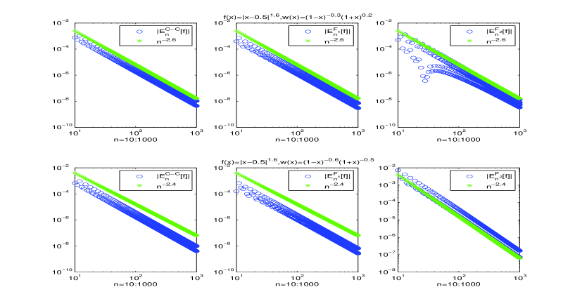
Fig. 4: The absolute errors for $n$-point Clenshaw-Curtis, Fejér’s first and second rules for $f(x)=|x-0.5|^{1.6}$ ($f\in X^{1.6}$) and $w(x)=(1-x)^{\alpha}(1+x)^{\beta}$ with $\alpha=-0.3$ and $\beta=0.2$ ($1$st row), and $\alpha=-0.6$ and $\beta=-0.5$ ($2$nd row), compared with $n^{-1-1.6}$ and $n^{-1.6-2-2\min(-0.6,-0.5)}$, respectively, for $n=10:1000$.

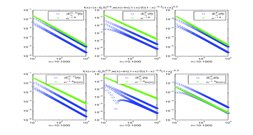
Fig. 5: The absolute errors for $n$-point Clenshaw-Curtis, Fejér’s first and second rules for $f(x)=|x-0.5|^{0.6}$ ($f\in X^{0.6}$) and $w(x)=\ln((1+x)/2)(1-x)^{\alpha}(1+x)^{\beta}$ with $\alpha=-0.3$ and $\beta=0.2$ compared with $n^{-1-0.6}$ ($1$st row), and $\alpha=-0.6$ and $\beta=-0.5$ ($2$nd row), compared with $n^{-0.6-2-2\min(-0.6,-0.5)}\ln n$, respectively, for $n=10:1000$.

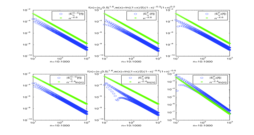
Fig. 6: The absolute errors for $n$-point Clenshaw-Curtis, Fejér’s first and second rules for $f(x)=|x-0.5|^{1.6}$ ($f\in X^{1.6}$) and $w(x)=\ln((1+x)/2)(1-x)^{\alpha}(1+x)^{\beta}$ with $\alpha=-0.3$ and $\beta=0.2$ compared with $n^{-1-1.6}$ ($1$st row), and $\alpha=-0.6$ and $\beta=-0.5$ ($2$nd row), compared with $n^{-1.6-2-2\min(-0.6,-0.5)}\ln n$, respectively, for $n=10:1000$.

4 Final remarks

The Peano kernel theorem provides a most useful representation of the quadrature error for the set of bounded variation functions (c.f. Brass [4], Brass and Petras [6] and Davis and Rabinowitz [11]). Based on the Peano kernel theorem and the estimates on the kernel function (c.f. Freud [19]), Brass and Petras [6] obtained the error bound for any quadrature with positive quadrature weights (also see Diethelm [12]).

Theorem 8.

(Brass and Petras [6]) Suppose $w(x)$ is a nonnegative and integrable weight function satisfies

(47) $$\sup_{-1\leq x\leq 1}w(x)(1-x^{2})^{1/2}<\infty,$$

and $E_{n}[{\cal P}_{n-1}]=0$ for any positive interpolatory quadrature formula $I_{n}$ with $n$ nodes, where ${\cal P}_{n-1}$ denotes the set of polynomials with degree less than $n-1$. If $f(x)$ has an absolutely continuous $(k-1)$st derivative $f^{(k-1)}$ on $[-1,1]$ (if $k\geq 1$) and a $k$th derivative $f^{(k)}$ of bounded variation $V_{k}$, then the quadrature error satisfies

(48) $$E_{n}[f]=O(n^{-k-1}).$$

Thus, $n$-point Gauss quadrature for the weight function satisfying (4.1) has the convergence rate (4.2). Particularly, the rate (4.2) can be achieved for functions of the form of

$$f^{(k)}(x)=\left\{\begin{array}[]{ll}0&\mbox{if $-1\leq x\leq\eta$}\\ M&\mbox{if $\eta<x\leq 1$}\end{array},\quad M\not=0,\right.$$

where $\eta$ is chosen so that $|K_{k+1}(\eta)|=\|K_{k+1}\|_{\infty}$ and $K_{k+1}$ is the $(k+1)$th Peano kernel function (c.f Brass and Petras [6, p. 87]). Then for this set of functions, the rate (4.2) is optimal.

However, the optimal convergence rate could be missed for such function which is of $k$th bounded variation with $\int_{-1}^{1}|f^{(k+1)}(x)|dx<\infty$ but the $(k+1)$th bounded variation does not exist, for example, $f_{*}^{(k)}(x)=\sqrt{1-x^{2}}$ (${\rm Var}(f_{*}^{(k)})<\infty$, $f_{*}\in X^{k+1}$), $f_{\gamma}^{(k)}(x)=|x-c|^{\gamma}$ (${\rm Var}(f_{\gamma}^{(k)})<\infty$, $f_{\gamma}\in X^{k+\gamma}$, $-1<c<1$, $0<\gamma<1$) and

$$f_{s}(x)=\left\{\begin{array}[]{ll}0&\mbox{if $-1\leq x\leq\xi$}\\ (x-\xi)_{+}^{s}&\mbox{if $\xi<x\leq 1$}\end{array},\right.\,\,-1<\xi<1,$$

where $s>0$ is a non-integer, ${\rm Var}(f_{s}^{(\lfloor s\rfloor)})<\infty$ and $f_{s}\in X^{s}$)

In addition, the convergence rate (48) can not be applied to the case

$${\displaystyle\sup_{-1<x<1}w(x)(1-x^{2})^{1/2}=\infty}.$$

Comparing Theorem 3.5 and Theorem 4.1, we see that the convergence orders in Theorem 3.5 on the above special functions by $n$-point Clenshaw-Curtis quadrature, Fejér’s first and second rules can be estimated higher than those by $n$-point Gauss quadrature given in Theorem 4.1 for $w(x)=(1-x)^{\alpha}(1+x)^{\beta}$ with $\alpha,\beta\geq-\frac{1}{2}$.

Nevertheless, numerical evidence shows that for Jacobi weight $w(x)=(1-x)^{\alpha}(1+x)^{\beta}$ ($\alpha,\beta>-1$), $n$-point Gauss quadrature enjoys the same convergence rate (3.21) as that for $n$-point Clenshaw-Curtis and Fejér’s quadrature, and is of approximately equal accuracy. For simplicity, here we only consider comparisons between Gauss and Clenshaw-Curtis quadrature for $f(x)=|x-0.5|^{s}$ ($f\in X^{s}$, $s=0.6,1.6$) and $w(x)=(1-x)^{\alpha}(1+x)^{\beta}$ with $\alpha=-0.3$ and $\beta=0.2$, and $\alpha=-0.6$ and $\beta=-0.5$, respectively: $n=10:1000$ (see Figure 4.1). Based on these numerical evidence, we put an open problem at the end.

Open problem. $n$-point Gauss quadrature enjoys the same convergence rate (3.21) for Jacobi weight $w(x)=(1-x)^{\alpha}(1+x)^{\beta}$ for $f\in X^{s}$.

Fig. 7: The absolute errors for $n$-point Gauss and Clenshaw-Curtis for $f(x)=|x-0.5|^{s}$ ($f\in X^{s}$) and $w(x)=(1-x)^{\alpha}(1+x)^{\beta}$: $n=10:1000$.

Acknowledgement. The author is grateful to Prof. Xiaojun Chen at Hong Kong Polytechnic University for her helpful comments and kind supports.

References

• [1] M. Abramowitz and I.A. Stegun, Handbook of Mathematical Functions, National Bureau of Standards, Washington, D.C., 1964.
• [2] I. Bogaert, B. Michiels and J. Fostier, $O(1)$ Computation of Legendre Polynomials and Gauss-Legendre Nodes and Weights for Parallel Computing, SIAM J. Sci. Comput., 34(2012) C83-C101.
• [3] J.P. Boyd, Chebyshev and Fourier Spectral Methods, Dover Publications, New York, 2000.
• [4] H. Brass, Quadraturverfahren. Vandenhoeck & Ruprecht, GΓΆttingen. 1977.
• [5] H. Brass and K. Petras, On a conjecture of D.B. Hunter, BIT, 37(1997) 227-231.
• [6] H. Brass and K. Petras, Quadrature Theory, Amer. Math. Soc., Providence, RI, 2011.
• [7] E.W. Cheney, Introduction to Approximation Theory, McGraw-Hill, New York, 1966.
• [8] C.W. Clenshaw and A.R. Curtis, A method for numerical integration on an automatic computer, Numer. Math., 2(1960) 197-205.
• [9] A.R. Curtis and P. Rabinowitz, On the Gaussian integration of Chebyshev polynomials, Math. Comp., 26(1972) 207-211.
• [10] G. Dahlquist and A. BjΓΆrck, Numerical Methods in Scientific Computing, SIAM, Philadelphia, 2007.
• [11] P.J. Davis and P. Rabinowitz, Methods of Numerical Integration, 2nd Ed., Academic Press, New York, 1984.
• [12] K. Diethelm, Error bounds for the numerical integration of functions with limited smoothness, SIAM J. Numer. Anal., 52(2)(2014) 877-879.
• [13] D. Elliott and D.F. Paget, Product-integration rules and their convergence, BIT, 16(1976) 32-40.
• [14] G. Evans, Praticle Numerical Integration, Wiley, Chichester, 1993.
• [15] L. FejΓ©r, Mechanische Quadraturen mit positiven Cotesschen Zahlen. Math. Z., 37(1933) 287-309.
• [16] K. FΓΆrster and K. Petras, On a problem proposed by H. Brass Concerning the remainder term in quadrature for convex functions, Numer. Math., 57(1990) 763-777.
• [17] K. FΓΆrster and K. Petras, Inequalities for the zeros of ultraspherical polynomials and Bessel functions, Z. Angew. Math. Mech., 73(1993) 232-236.
• [18] L. Fox and I.B. Parker, Chebyshev Polynomials in Numerical Analysis, Oxford University Press, London, 1968.
• [19] G. Freud, Über einseitige Approximation durch Polynome, I, Acta. Sci. Math., 16(1959) 12-28.
• [20] L. Gatteschi, New inequalities for the zeros of Jacobi polynomials, SIAM J. Math. Anal., 18(1987) 1549-1562.
• [21] W. Gautschi, Construction of Gauss-Christoffel quadrature formulas, Math. Comp., 22(1968) 251-270.
• [22] A. Glaser, X. Liu, V. Rokhlin, A fast algorithm for the calculation of the roots of special functions, SIAM J. Sci. Comput., 29(2007) 1420-1438.
• [23] N. Hale and A. Townsend, Fast and accurate computation of Gauss-Legendre and Gauss-Jacobi quadrature nodes and weights, SIAM J. Sci. Comput., 35(2013) A652-A674.
• [24] H. O’Hara and F. Smith, Error estimation in the Clenshaw-Curtis quadrature formula, Comp. J., 11(1968) 213-219.
• [25] J. Hesthaven, S. Gottlieb and D. Gottlieb, Spectral Methods for Time-Dependent Problems, Cambridge University Press, Cambridge, 2007.
• [26] P.K. Kythe and M.R. SchΓ€ferkotter, Handbook of Computational Methods for Integration, Chapman and Hall/CRC, New York, 2005.
• [27] M. Lighthill, Fourier analysis and generalized functions, Cambridge University Press, Cambridge, 1959.
• [28] S.C. Malik and Savita Arora, Mathematical Analysis, New Age International, New Delhi, 1992.
• [29] A. Zygmund, Trigonometric series, Vols. 1 and 2, Cambridge University Press, 1959.
• [30] K. Petras, Gaussian integration of Chebyshev polynomials and analytic functions, Numer. Alg., 10(1995) 187-202.
• [31] R. Piessens and M. Branders, The evaluation and application of some modified moments, BIT, 13(1973) 443-450.
• [32] R.D. Riess and L.W. Johnson, Error esitmates for Clenshaw-Curtis quadrature, Numer. Math., 18(1972) 345-353.
• [33] I.H Sloan, On the numerical evaluation of singular integrals, BIT, 18(1978) 91-102.
• [34] I.H. Sloan and W.E. Smith, Product-integration with the Clenshaw-Curtis and related points, Numer. Math., 30(1978) 415-428.
• [35] I. H. Sloan and W.E. Smith, Product integration with the Clenshaw-Curtis points: implementation and error estimates, Numer. Math., 34(1980) 387-401.
• [36] A. Sommariva, Fast construction of FejΓ©r and Clenshaw-Curtis rules for general weight functions, Comput. Math. Appl., 65(2013) 682-693.
• [37] G. SzegΓΆ, Orthogonal Polynomial, American Mathematical Society, Providence, Rhode Island, 1939.
• [38] L.N. Trefethen, Is Gauss quadrature better than Clenshaw-Curtis?, SIAM Review, 50(2008) 67-87.
• [39] L.N. Trefethen, Approximation Theory and Approximation Practice, SIAM, Philadelphia, 2013.
• [40] L.N. Trefethen and others, Chebfun Version 4.2, The Chebfun Development Team, 2011, http://www.maths.ox.ac.uk/chebfun/.
• [41] J. Waldvogel, Fast construction of the FejΓ©r and Clenshaw-Curtis quadrature rules, BIT, 46(2006) 195-202.
• [42] H. Wang and S. Xiang, On the convergence rates of Legendre approximation, Math. Comp., 81(2012) 861-877.
• [43] S. Xiang, X. Chen and H. Wang, Error bounds in Chebyshev points, Numer. Math., 116(2010) 463-491.
• [44] S. Xiang, On error bounds for orthogonal polynomial expansions and Gauss-type quadrature, SIAM J. Numer. Anal., 50(2012) 1240-1263.
• [45] S. Xiang and F. Bornemann, On the convergence rates of Gauss and Clenshaw-Curtis quadrature for functions of limited regularity, SIAM J. Numer. Anal., 50(2012) 2581-2587.
• [46] S. Xiang, G. He and H. wang, On Fast Implementation of Clenshaw-Curtis and FejΓ©r-type Quadrature Rules, arXiv:1311.0445, 2013.