ON OBSTACLE NUMBERS

The obstacle number is a new graph parameter introduced by Alpert, Koch, and Laison (2010). Mukkamala et al. (2012) show that there exist graphs with $n$ vertices having obstacle number in $\Omega(n/\log n)$. In this note, we up this lower bound to $\Omega(n/(\log\log n)^{2})$. Our proof makes use of an upper bound of Mukkamala et al. on the number of graphs having obstacle number at most $h$ in such a way that any subsequent improvements on their upper bound will improve our lower bound.

1 Introduction

The obstacle number is a new graph parameter introduced by Alpert, Koch, and Laison [2]. Let $G=(V,E)$ be a graph, let $\varphi:V\to\mathbb{R}^{2}$ be a one-to-one mapping of the vertices of $G$ onto $\mathbb{R}^{2}$, and let $S$ be a set of connected subsets of $\mathbb{R}^{2}$. The pair $(\varphi,S)$ is an obstacle representation of $G$ when, for every pair of vertices $u,w\in V$, the edge $uw$ is in $E$ if and only if the open line segment with endpoints $\varphi(u)$ and $\varphi(w)$ does not intersect any obstacle in $S$. An obstacle representation $(\varphi,S)$ is an $h$-obstacle representation if $|S|=h$. The obstacle number of a graph $G$, denoted by $\operatorname{obs}(G)$, is the minimum value of $h$ such that $G$ has an $h$-obstacle representation.

Figure 1 shows a surprising example of a 1-obstacle representation of the $5\times 5$ grid graph, $G_{5\times 5}$, that was given to us by Fabrizio Frati. In this figure, the single obstacle is drawn as a shaded region. Since at least one obstacle is clearly necessary to represent any graph other than a complete graph, this proves that $\operatorname{obs}(G_{5\times 5})=1$. (A similar drawing can be used to show that the $a\times b$, grid graph has obstacle number 1, for any integers $a,b>1$.)

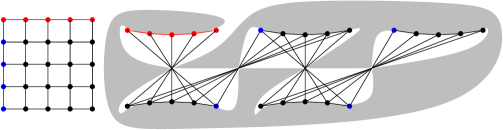
Figure 1: The $5\times 5$ grid graph has obstacle number 1.

Since their introduction, obstacle numbers have generated significant research interest [6, 11, 12, 13, 14, 15, 16]. A fundamental—and far from answered—question about obstacle numbers is that of determining the worst-case obstacle number,

$$w(n)=\max\{\operatorname{obs}(G):\mbox{$G$ is a graph with $n$ vertices}\}\enspace,$$

of a graph with $n$ vertices.

For a graph $G=(V,E)$, we call elements of $\binom{V}{2}\setminus E$ non-edges of $G$. The worst-case obstacle number $w(n)$ is obviously upper-bounded by $\binom{n}{2}\in O(n^{2})$ since, by mapping the vertices of $G$ onto a point set in sufficiently general position, one can place a small obstacle—even a single point—on the mid-point of each non-edge of $G$. No upper-bound on $w(n)$ that is asymptotically better than $O(n^{2})$ is known.

More is known about lower-bounds on $w(n)$. Alpert et al. initially show that the worst-case obstacle number is $\Omega(\sqrt{\log n/\log\log n})$ and posed as an open problem the question of determining if $w(n)\in\Omega(n)$. Mukkamala et al. [13] showed that $w(n)\in\Omega(n/\log^{2}n)$ and Mukkamala et al. [12] later increased this to $w(n)\in\Omega(n/\log n)$. In the current paper, we up the lower-bound again by proving the following theorem:

Theorem 1.

For every integer $n>0$, $w(n)\in\Omega(n/(\log\log n)^{2})$, i.e., there exist graphs, $G$, with $n$ vertices and $\operatorname{obs}(G)\in\Omega(n/(\log\log n)^{2})$.

The proof of Theorem 1 makes use of an upper bound of Mukkamala et al. [12, Theorem 1] on the number of graphs having obstacle number at most $h$ in such a way that any subsequent improvements on their upper bound will result in an improved lower bound on $w(n)$.

2 The Proof

Our proof strategy is an application of the probabilistic method [1]. We will show that, for a random graph, $G$, with a fixed embedding, the probability, $p$, that this embedding allows for an obstacle representation with few obstacles is extremely small. We will then show that the number, $N$, of combinatorially distinct embeddings is not too big. Small and big in this case are defined so that $pN<1$. Therefore, by the union bound, there exists at least one graph, $G^{\prime}$, that has no embedding that allows for an obstacle representation with few obstacles. In other words, $\operatorname{obs}(G^{\prime})$ is large.

2.1 A Random Graph with a Fixed Embedding

We make use of the following theorem, due to Mukkamala, Pach, and Pálvölgyi [12, Theorem 1] about the number of $n$ vertex graphs with obstacle number at most $h$:

Theorem 2 (Mukkamala, Pach, and Pálvölgyi 2012).

For any $h\geq 1$, the number of graphs having $n$ vertices and obstacle number at most $h$ is at most $2^{O(hn\log^{2}n)}$.

Recall that an Erdös-Renyi random graph $G_{n,\frac{1}{2}}$ is a graph with $n$ vertices and each pair of vertices is chosen as an edge or non-edge with equal probability and independently of every other pair of vertices [4]. The following lemma shows that, for random graphs, a fixed embedding is very unlikely to yield an obstacle representation with few obstacles.

Lemma 1.

Let $G=(V,E)$ be an Erdös-Rényi random graph $G_{n,\frac{1}{2}}$, let $\varphi\colon V\to\mathbb{R}^{2}$ be a one-to-one mapping that is independent of the choices of edges in $G$, and let $(\varphi,S)$ be an obstacle representation of $G$ using the minimum number of obstacles (subject to $\varphi$). Then, for any constant $c>0$,

$$\Pr\{|S|\in\Omega(n/(\log\log n)^{2})\geq 1-e^{-\Omega(cn\log n)}\enspace.$$

Proof.

Let $P\subset\mathbb{R}^{2}$ denote the image of $\varphi$. Fix some integer $k$ to be specified later and first consider some arbitrary subset $P^{\prime}\subset P$ of $k$ points and let $G^{\prime}=(V^{\prime},E^{\prime})$ be the subgraph of $G$ induced by the set $V^{\prime}=\{\varphi^{-1}(x):x\in P^{\prime}\}$ of vertices that are mapped by $\varphi$ to $P^{\prime}$. Applying Theorem 2 with $n=k$ and $h=\alpha k/\log^{2}k$, we obtain

$$\Pr\{\operatorname{obs}(G^{\prime})\leq\alpha k/\log^{2}k\}\leq\frac{2^{O(\alpha k^{2})}}{2^{\binom{k}{2}}}=e^{-\Omega(k^{2})}\enspace,$$ (1)

for a sufficiently small constant $\alpha>0$. Note that, if $\operatorname{obs}(G^{\prime})\geq h$, then, in the obstacle representation $(\varphi,S)$, there must be at least $h-1$ obstacles of $S$ that are contained in the convex hull of $P^{\prime}$.

Without loss of generality assume that no two points in $P$ have the same x-coordinate and denote the points in $P$ by $x_{0},\ldots,x_{n-1}$ by increasing order of x-coordinate. Let $m=\lfloor n/k\rfloor$ and consider the point sets $P^{\prime}_{0},\ldots,P^{\prime}_{m-1}$, where

$$P_{i}^{\prime}=\{x_{ik},x_{ik+1},\ldots,x_{ik+k-1}\}\enspace.$$

That is, $P_{0}^{\prime},\ldots,P_{m-1}^{\prime}$ are determined by vertical slabs, $s_{0},\ldots,s_{m-1}$ that each contain $k$ points. Equation (1) shows that, with probability at least $1-2^{-\Omega(k^{2})}$, the obstacle number of the subgraph that maps to $P^{\prime}_{i}$ is $\Omega(k/\log^{2}k)$. If this occurs, then $S$ has $\Omega(k/\log^{2}k)$ obstacles that are completely contained in the slab $s_{i}$. These obstacles are therefore disjoint from any other obstacles contained in any other slab $s_{j}$, $j\neq i$.

We are proving a lower bound on the number of obstacles, so we are worried about the case where the number of slabs that do not completely contain at least $\alpha k/\log^{2}k$ obstacles exceeds $m/2$. The number of slabs, $M$, not containing at least $\alpha k/\log^{2}k$ obstacles is dominated by a binomial$(m,2^{-\Omega(k^{2})})$ random variable. Using Chernoff’s bound on the tail of a binomial random variable, we have that Pr{M ≥m/2} & = Pr{M≥(1+δ)μ} (where $\mu=me^{-ck^{2}}$ and $\delta=e^{ck^{2}-1}-1$)
≤(eδ(1+δ)1+δ)^μ
= (eeck2(eck2-1)eck2-1)^me^-ck^2
= (eeck2e(ck2-1)eck2-1)^me^-ck^2
= emem(ck2-1)eck2-1e-ck2
= emem(ck2-1)/e
= e^-Ω(mk^2)  . Taking $k=\sqrt{c}\log n$ and recalling that $m=\lfloor n/k\rfloor$, we obtain the desired result. In particular,

$$|S|\geq\Omega\left(\left(k/\log^{2}k\right)\times m\right)=\Omega\left(n/(\log\log n)^{2}\right)$$

with probability at least

$$1-e^{-\Omega(mk^{2})}=1-e^{-\Omega(cn\log n)}\enspace.\qed$$

We have completed the first step in our application of the probabilistic method. Lemma 1 shows that the probability, $p$, that a particular embedding of the random graph $G$ is able to yield an obstacle representation with $o(n/(\log\log n)^{2})$ obstacles is extremely small. The remaining difficulty is establishing a sufficiently strong upper-bound on $N$, the number of embeddings of $G$. In actuality, the number of embeddings is uncountable. However, we are interested in the number of “combinatorially distinct” embeddings. In particular, we would like to partition the set of embeddings into equivalence classes such that, within each equivalence class, the minimum number of obstacles in an obstacle representation remains the same.

Classifying embeddings (i.e., labelled sets of $n$ points) into combinatorially distinct equivalence classes has been considered previously. Several definitions of equivalence exist, including oriented matroid (a.k.a., chirotope) equivalence [3, 5], semispace equivalence [9], order equivalence [8], and combinatorial equivalence [7, 9]. For the latter two definitions of equivalence, the number of distinct (equivalence classes of) point sets is $e^{O(n\log n)}$ [10].

Unfortunately, neither order types nor combinatorial-types are sufficient for answering questions about obstacle representations. To see this, consider the two embeddings of the same graph shown in Figure 2. These two embeddings have the same order type and the same combinatorial type. However, the embedding on the right admits an obstacle representation with one obstacle, while the one on the left requires two obstacles. To see why this is so, observe that each embedding needs an obstacle on the outer face (shown). For the embedding on the right, this single obstacle is sufficient, but the embedding on the left needs an additional obstacle inside one of the inner faces.

Figure 2: Order type and combinatorial type are insufficient to determine the number of obstacles needed in an obstacle representation. The yellow segment represents a non-edge.

2.2 Super-Order Types

We now define an equivalence relation on point sets that is strong enough for our purposes. Consider a sextuple $T=\langle a_{1},a_{2},b_{1},b_{2},c_{1},c_{2}\rangle$ of points such that

1. $a_{1}\neq a_{2}$, $b_{1}\neq b_{2}$, $c_{1}\neq c_{2}$,

2. $\{a_{1},a_{2}\}\neq\{b_{1},b_{2}\}$, $\{b_{1},b_{2}\}\neq\{c_{1},c_{2}\}$, $\{c_{1},c_{2}\}\neq\{a_{1},a_{2}\}$, and

3. $\{a_{1},a_{2}\}\cap\{b_{1},b_{2}\}\cap\{c_{1},c_{2}\}=\emptyset$.

We call a sextuple $T$ with this property an admissible sextuple. Let $A$ denote the directed line through $a_{1}$ and $a_{2}$ that is directed from $a_{1}$ towards $a_{2}$. Define $B$ and $C$ similarly, but with respect to $b_{1},b_{2}$ and $c_{1},c_{2}$, respectively. We say that the sextuple, $T$, is degenerate if

1. any of $A$, $B$, or $C$ is vertical;

2. $A$ is parallel to $B$ or to $C$; or

3. $A$, $B$, and $C$ contain a common point.

We define the type, $\sigma(T)$, of $T$ as

$$\sigma(T)=\left\{\begin{array}[]{rl}-1&\text{if$A\cap B$comesbefore$A\cap C$on$A$.}\\ 0&\text{if$T$isdegenerate}\\ +1&\text{otherwise($A\cap B$comesafter$A\cap C$on$A$).}\end{array}\right.$$

(See Figure 3.) Let $\langle\langle i_{1,\ell},i_{2,\ell},j_{1,\ell},j_{2,\ell},k_{1,\ell},k_{2,\ell}\rangle:\ell\in\{1,\ldots,r\}\rangle$ be any sequence that lists the admissible sextuples of the index set $\{1,\ldots,n\}$. Note that $r<\binom{n}{2}^{3}$. The super-order type of a sequence $P=\langle x_{1},\ldots,x_{n}\rangle$ of $n$ distinct points is the sequence

$$\sigma(P)=\left\langle\sigma\left(x_{i_{1,\ell}},x_{i_{2,\ell}},x_{j_{1,\ell}},x_{j_{2,\ell}},x_{k_{1,\ell}},x_{k_{2,\ell}}\right):\ell\in\left\{1,\ldots,r\right\}\right\rangle\enspace.$$

Finally, we say that super-order type is simple if it contains no zeros and a sequence of points is simple if its super-order type is simple. The following lemma shows that super-order types are sufficient for answering questions about obstacle representations.

-1	1

0	0	0

Figure 3: The three cases of three lines defined by 6 points that can occur in the super-order type.

Lemma 2.

Let $G$ be a graph with vertex set $V=\{1,\ldots,n\}$ and let $\varphi_{1}\colon V\to\mathbb{R}^{2}$ and $\varphi_{2}\colon V\to\mathbb{R}^{2}$ be two embeddings of $G$ such that $\langle\varphi_{1}(1),\ldots,\varphi_{1}(n)\rangle$ and $\langle\varphi_{2}(1),\ldots,\varphi_{2}(n)\rangle$ have the same super-order type. Then, if $G$ has an $h$-obstacle representation $(\varphi_{1},S_{1})$ then it also has $h$-obstacle representation $(\varphi_{2},S_{2})$.

Proof.

Consider the two plane graphs $G_{1}$ and $G_{2}$ obtained by adding a vertex where any two edges cross in the embedding $\phi_{1}$, respectively, $\phi_{2}$ cross. The fact that $\langle\varphi_{1}(1),\ldots,\varphi_{1}(n)\rangle$ and $\langle\varphi_{2}(1),\ldots,\varphi_{2}(n)\rangle$ have the same super-order type implies that $G_{1}$ and $G_{2}$ are two combinatorially equivalent drawings of the same planar graph. Without loss of generality, we can assume that each obstacle $X_{1}\in S_{1}$ is an open polygon whose boundary is the face, $f_{1}$, of $G_{1}$ that contains $X_{1}$. For each such obstacle, we create an obstacle, $X_{2}\in S_{2}$, whose boundary is the face $f_{2}$ of $G_{2}$ that corresponds to $f_{1}$.

All that remains is to verify that an edge $uw$ is in $G$ if and only if the segment with endpoints $\varphi_{2}(u)$ and $\varphi_{2}(w)$ does not intersect any obstacle in $S_{2}$. By construction, no edge of the embedding $\varphi_{2}$ of $G$ intersects any obstacle in $S_{2}$. Because $P_{1}$ and $P_{2}$ have the same super-order type it is easy to verify that, for every non-edge $uw$ of $G$, the segment $\varphi_{2}(u)\varphi_{2}(w)$ intersects some obstacle in $S_{2}$. (Indeed, $\varphi_{2}(u)\varphi_{2}(w)$ intersects the obstacles of $S_{2}$ corresponding to those in $S_{1}$ intersected by $\varphi_{1}(u)\varphi_{1}(w)$.) That is, $(\varphi_{2},S_{2})$ is an obstacle representation of $G$ using $h=|S_{1}|$ obstacles, as required. ∎

The next lemma shows that we can restrict our attention to embeddings onto simple point sets.

Lemma 3.

If a graph $G$ with vertex set $V=\{1,\ldots,n\}$ has an $h$-obstacle representation $(\varphi,S)$, then $G$ has an $h$-obstacle representation $(\varphi^{\prime},S^{\prime})$ in which the $\langle\varphi(1),\ldots,\varphi(n)\rangle$ is a simple point sequence.

Proof.

We first note that, by rotation, we can assume that no two points in the image of $\varphi$ have the same x-coordinate. Therefore, any degenerate sextuple in the image of $\varphi$ is not the result of a vertical line through two points in the sextuple. Instead, each degenerate sextuple is the result of two parallel lines or of three lines passing through a common point.

By growing the obstacles in $S$ into maximal open sets and then shrinking them slightly, we may assume that each obstacle in $S$ is an open set that is at some positive distance $\epsilon>0$ from each line segment $\varphi(u)\varphi(w)$ joining the two endpoints of each edge $uw$ in $G$. Call this new set of obstacles $S^{\prime}$. We say that two points $a$ and $b$ are visible if the open line segment with endpoints $a$ and $b$ does not intersect any obstacle in $S^{\prime}$, otherwise we say that $a$ and $b$ are invisible.

If the image of $\varphi$ is a non-simple point set, then some point $a_{1}=\varphi(u)$ is involved in a degenerate sextuple $T=(a_{1},a_{2},b_{1},b_{2},c_{1},c_{2})$. Then there exists a sufficiently small perturbation of $a_{1}$ that moves it to a new location $a_{1}^{\prime}$ that simultaneously

1. eliminates all the degenerate sextuples that include $a_{1}$;

2. does not change the type of any non-degenerate sextuple;

3. does not result in any point $b=\varphi(w)$ that is visible to $a_{1}$ being invisible to $a_{1}^{\prime}$; and

4. does not result in any point $b=\varphi(w)$ that is invisible to $a_{1}$ being visible to $a_{1}^{\prime}$.

Note that the first two properties ensure that, by moving $a_{1}$ to $a_{1}^{\prime}$, the number of degenerate sextuples decreases. The last three properties ensure that the resulting embedding along with the obstacle set $S^{\prime}$ is an obstacle representation of $G$. We can easily verify that such a point $a_{1}^{\prime}$ exists because

1. For each degenerate sextuple that includes $a_{1}$ there are only a constant number of directions $(a-a^{\prime})/\|a-a^{\prime}\|$ that preserve the degeneracy of that sextuple.

2. Changing the type of a non-denerate sextuple involving $a_{1}$ requires moving $a_{1}$ by some distance $\delta>0$; we can ensure that our perturbation moves $a_{1}$ by less than $\delta$.

3. All obstacles are at distance $\epsilon>0$ from the edges of the embedding. We can ensure that the perturbation moves $a_{1}$ by less than $\epsilon$.

4. All obstacles are open sets, so every non-edge intersects the interior of one or more obstacles. By making the perturbation of $a_{1}$ sufficiently small, each such non-edge continues to intersect the interiors of the same obstacles.

The preceding perturbation step can be repeated until no degenerate sextuples remain to obtain the desired $h$-obstacle representation $(\varphi^{\prime},S^{\prime})$. ∎

What remains is to show that $N$, the number of super-order types corresponding to point sets of size $n$ is not too big. Luckily, the methods used by Goodman and Pollack [10] to upper bound the numbers of order types and combinatorial types generalize readily to super-order types. The proof of the following result is given in Appendix A.

Lemma 4.

The number of sequences in $\{-1,{+1}\}^{r}$ that are the super-order type of some simple point sequence of length $n$ is $e^{O(n\log n)}$.

2.3 Proof of Theorem 1

For completeness, we now spell out the proof of Theorem 1.

Proof of Theorem 1.

Let $G$ be an Erdös-Rényi random graph with $n$ vertices. We say that the (point set which is the) image of $\varphi$ in an obstacle representation $(\varphi,S)$ supports the obstacle representation. Fix some simple super-order type on $n$ points. By Lemma 2, all point sets with this super-order type support an obstacle representation of $G$ with $o(n/(\log\log n)^{2})$ obstacles or none of them do. By Lemma 1, the probability that all of them do is at most $p\leq e^{-cn\log n}$ for every constant $c>0$. By the union bound and Lemma 4 the probability that there is any simple super-order type—and therefore any simple point set—that supports an obstacle representation of $G$ with $o(n/(\log\log n)^{2})$ obstacles is

$$\hat{p}=p\cdot e^{O(n\log n)}=e^{-cn\log n}\cdot e^{O(n\log n)}<1$$

for a sufficiently large constant $c$. Therefore, with probability $1-\hat{p}>0$, there is no simple point set that supports an obstacle representation of $G$ using $o(n/(\log\log n)^{2})$ obstacles. We deduce that there exists some some graph, $G^{\prime}$, with this property. Finally, Lemma 3 implies that we can ignore the restriction to simple point sets and deduce that $\operatorname{obs}(G^{\prime})\in\Omega(n/(\log\log n)^{2})$. ∎

3 Remarks

Our proof of Theorem 1 relates the problem of counting the number of $n$-vertex graphs with obstacle number at most $h$ to the problem of determining the worst-case obstacle number of a graph with $n$ vertices. Currently, we use Mukkamala et al.’s Theorem 2, which proves an upper-bound of $e^{O(hn\log^{2}n)}$ on the number of $n$ vertex graphs with obstacle number at most $h$. Interestingly, their argument is an encoding argument, which shows that any such graph can be encoded as the order type of a set of $O(hn\log n)$ points followed by a list of the points in this set that make up the vertices of the (polygonal) obstacles. Their argument needs only order types (as opposed to super-order types) since the point set that they specify includes the vertices of the obstacles.

Any improvement on the upper-bound for the counting problem will immediately translate into an improved lower-bound on the worst-case obstacle number. In particular, let $f(h,n)$ denote the number of $n$-vertex graphs with obstacle number at most $h$ and let $\hat{h}(n)=\max\{h:f(h,n)\leq 2^{n^{2}/4}\}$. Then our proof technique shows that there exist graphs with obstacle number at least $n\hat{h}(c\log n)/(c\log n)$. (Theorem 2 shows that $\hat{h}(c\log n)\in\Omega(\log n/(\log\log n)^{2})$.)

We note that our technique gives an improved lower bound until someone is able to prove that $\hat{h}(n)\in\Omega(n)$. At this point, a simple argument (see [13, Theorem 3]) shows that there exists graphs with obstacle number at least $\hat{h}(n)$.

We conjecture that improved upper-bounds on $f(h,n)$ that reduce the dependence on $h$ are the way forward:

Conjecture 1.

$f(h,n)\leq 2^{g(n)\cdot o(h)}$, where $g(n)\in O(n\log^{2}n)$.

In support of this conjecture, we observe that an upper bound of the form $f(1,n)\leq 2^{g(n)}$ is sufficient to give the crude upper bound $f(h,n)\leq 2^{h\cdot g(n)}$ since any graph with an $h$-obstacle representation is the common intersection of $h$ graphs that each have a 1-obstacle representation. That is, if $\operatorname{obs}(G)\leq h$, then there exists $E_{1},\ldots,E_{h}$ such that $G=(V,\bigcap_{i=1}^{h}E_{i})$ and $\operatorname{obs}(V,E_{i})=1$ for all $i\in\{1,\ldots,h\}$. This seems like a very crude upper bound in which many graphs are counted multiple times. Conjecture 1 asserts that this argument overestimates the dependence on $h$.

Appendix A Proof of Lemma 4

Proof of Lemma 4.

For a point, $p$, let $\mathsf{x}(p)$ and $\mathsf{y}(p)$ denote the x- and y-coordinate, respectively, of $p$. Consider what it means for a sextuple $T=(a_{1},a_{2},b_{1},b_{2},c_{1},c_{2})$, which defines three lines $A$, $B$, and $C$, to be degenerate. This can occur, for example, if $A$ and $B$ are parallel. The lines $A$ and $B$ are parallel if and only if

$$\mathsf{x}(a_{1}-a_{2})\cdot\mathsf{y}(b_{1}-b_{2})-\mathsf{x}(b_{1}-b_{2})\cdot\mathsf{y}(a_{1}-a_{2})=0\enspace.$$

(This formula is a formalization of the less precise statement “the slopes of $A$ and $B$ are the same.”) Observe that the preceding equation is a polynomial in $a_{1},a_{2},b_{1},b_{2}$ of degree 2.

Next, consider the case where $T$ is degenerate because $A$, $B$, and $C$ intersect in a common point or because one of $A$, $B$, or $C$ is vertical. This occurs if and only if the following determinant is undefined or equal to zero:

$$\left|\begin{array}[]{lll}\mathsf{y}(a_{1})-\mathsf{x}(a_{1})\left(\frac{\mathsf{y}(a_{1}-a2)}{\mathsf{x}(a_{1}-a_{2})}\right)&\frac{\mathsf{y}(a_{1})-\mathsf{y}(a_{2})}{\mathsf{x}(a_{1})-\mathsf{x}(a_{2})}&1\\ \mathsf{y}(b_{1})-\mathsf{x}(b_{1})\left(\frac{\mathsf{y}(b_{1}-b2)}{\mathsf{x}(b_{1}-b_{2})}\right)&\frac{\mathsf{y}(b_{1})-\mathsf{y}(b_{2})}{\mathsf{x}(b_{1})-\mathsf{x}(b_{2})}&1\\ \mathsf{y}(c_{1})-\mathsf{x}(c_{1})\left(\frac{\mathsf{y}(c_{1}-c2)}{\mathsf{x}(c_{1}-c_{2})}\right)&\frac{\mathsf{y}(c_{1})-\mathsf{y}(c_{2})}{\mathsf{x}(c_{1})-\mathsf{x}(c_{2})}&1\\ \end{array}\right|\enspace.$$ (2)

(The values in this matrix are the $\mathsf{y}$-intercepts and slopes of the lines $A$, $B$, and $C$.) Multiplying the matrix in (2) by

$$\mathsf{x}(a_{1}-a_{2})\cdot\mathsf{x}(b_{1}-b_{2})\cdot\mathsf{x}(c_{1}-c_{2})$$

yields a polynomial of degree $6$ in the six variables $a_{1},a_{2},b_{1},b_{2},c_{1},c_{2}$ that is equal to zero if and only if $A$, $B$, and $C$ contain a common point or one of $A$, $B$, or $C$ is vertical. (Recall that $\det(cA)=c^{r}\cdot\det(A)$ when $A$ is a $r\times r$ matrix.)

For the remainder of the proof, we proceed exactly as in [10]. We can treat any sequence of $n$ points in $\mathbb{R}^{2}$ as a single point in $\mathbb{R}^{2n}$. Applying the preceding conditions for determining the degeneracy to each of the $O(n^{6})$ admissible sextuples of points results in a set of $O(n^{6})$ polynomials in $2n$ variables, each of constant degree. By multiplying these polynomial together, we obtain a single polynomial, $P^{*}$, in $2n$ variables and having degree $d\in O(n^{6})$. If $X\subset\mathbb{R}^{2n}$ is the zero set of $P^{*}$, then $\mathbb{R}^{2n}\setminus X$ has at most $(2+d)^{2n}=e^{O(n\log n)}$ connected components [10, Lemma 2].

Observe that $X$ corresponds exactly to the set of non-simple point sequences and observe that a sextuple of points can not be moved continuously so that its type goes from $-1$ to $+1$, or vice versa, without its type becoming $0$ at some point during the movement. In particular, it is not possible to change the super-order type of a simple point sequence without going through a non-simple super-order type. Thus, within each component, $C$, of $\mathbb{R}^{2n}\setminus X$, the super-order type corresponding to every point in $C$ is the same. We conclude that the number of super-order types of simple point sequences is at most the number of components of $\mathbb{R}^{2n}\setminus X$, which is $e^{O(n\log n)}$, as required. ∎

Authors

Vida Dujmović. School of Mathematics and Statistics and Department of Systems and Computer Engineering, Carleton University

Pat Morin. School of Computer Scence, Carleton University

References

- [1] N. Alon and J. H. Spencer. The Probabilistic Method. John Wiley & Sons, Hoboken, third edition, 2008.
- [2] H. Alpert, C. Koch, and J. D. Laison. Obstacle numbers of graphs. Discrete & Computational Geometry, 44(1):223–244, 2010.
- [3] R. G. Bland and M. L. Vergnas. Orientability of matroids. J. Comb. Theory, Ser. B, 24(1):94–123, 1978.
- [4] P. Erdös and A. Rényi. On random graphs. Publicationes Mathematicae, 6:290–297, 1959.
- [5] J. Folkman and J. Lawrence. Oriented matroids. J. Combin. Theory Ser. B, 25:199–236, 1978.
- [6] R. Fulek, N. Saeedi, and D. Sariöz. Convex obstacle numbers of outerplanar graphs and bipartite permutation graphs. CoRR, abs/1104.4656, 2011.
- [7] J. E. Goodman. On the combinatorial classification of nondegenerate configurations in the plane. J. Comb. Theory, Ser. A, 29(2):220–235, 1980.
- [8] J. E. Goodman and R. Pollack. Multidimensional sorting. SIAM J. Comput., 12(3):484–507, 1983.
- [9] J. E. Goodman and R. Pollack. Semispaces of configurations, cell complexes of arrangements. J. Comb. Theory, Ser. A, 37(3):257–293, 1984.
- [10] J. E. Goodman and R. Pollack. Upper bounds for configurations and polytopes in r. Discrete & Computational Geometry, 1:219–227, 1986.
- [11] M. P. Johnson and D. Sariöz. Computing the obstacle number of a plane graph. CoRR, abs/1107.4624, 2011.
- [12] P. Mukkamala, J. Pach, and D. Pálvölgyi. Lower bounds on the obstacle number of graphs. Electr. J. Comb., 19(2):P32, 2012.
- [13] P. Mukkamala, J. Pach, and D. Sariöz. Graphs with large obstacle numbers. In D. M. Thilikos, editor, WG, volume 6410 of Lecture Notes in Computer Science, pages 292–303, 2010.
- [14] J. Pach and D. Sariöz. Small -colorable graphs without 1-obstacle representations. CoRR, abs/1012.5907, 2010.
- [15] J. Pach and D. Sariöz. On the structure of graphs with low obstacle number. Graphs and Combinatorics, 27(3):465–473, 2011.
- [16] D. Sariöz. Approximating the obstacle number for a graph drawing efficiently. In CCCG, 2011.