Regularized Reconstruction of a Surface from its Measured Gradient Field

Abstract

This paper presents several new algorithms for the regularized reconstruction of a surface from its measured gradient field. By taking a matrix-algebraic approach, we establish general framework for the regularized reconstruction problem based on the Sylvester Matrix Equation. Specifically, Spectral Regularization via Generalized Fourier Series (e.g., Discrete Cosine Functions, Gram Polynomials, Haar Functions, etc.), Tikhonov Regularization, Constrained Regularization by imposing boundary conditions, and regularization via Weighted Least Squares can all be solved expediently in the context of the Sylvester Equation framework. State-of-the-art solutions to this problem are based on sparse matrix methods, which are no better than $\mathcal{O}\!\left(n^{6}\right)$ algorithms for an $m\times n$ surface. In contrast, the newly proposed methods are based on the global least squares cost function and are all $\mathcal{O}\!\left(n^{3}\right)$ algorithms. In fact, the new algorithms have the same computational complexity as an SVD of the same size. The new algorithms are several orders of magnitude faster than the state-of-the-art; we therefore present, for the first time, Monte-Carlo simulations demonstrating the statistical behaviour of the algorithms when subject to various forms of noise. We establish methods that yield the lower bound of their respective cost functions, and therefore represent the “Gold-Standard” benchmark solutions for the various forms of noise. The new methods are the first algorithms for regularized reconstruction on the order of megapixels, which is essential to methods such as Photometric Stereo.

1 Introduction

Surface reconstruction from a gradient field is an important problem, not only in Imaging, but in the Physical Sciences in general; it is essential to many applications such as Photometric Stereo woodham1980 , Seismic Imaging robein , as well as the more general problem of the numerical solution of Partial Differential Equations. The reconstruction from gradients problem can be considered to be an inverse problem, that is, inversion of the process of differentiation. The difficulty arises in the fact that if a gradient field is corrupted by Gaussian noise, it is generally no longer integrable. To make matters worse, the Gaussian noise is itself to some degree integrable, which introduces bias into the solution. It is generally known that the surface can be reconstructed up to a constant of integration, whereby a global least squares solution accomplishes this Harker2008c . However, when different forms of noise are present (e.g., lighting variations in Photometric Stereo, or gross outliers), the least squares solution is no longer optimal in the maximum likelihood sense. To suppress such varied types of noise, some form of regularization is required on the solution to the reconstruction problem. More importantly, a mathematically sound and efficient solution to this problem is fundamental to obtaining useable results from surface measurement via Photometric Stereo. In this paper, we derive several new methods which incorporate state-of-the-art regularization techniques into the surface reconstruction problem. In Harker2008c , it was first shown that the global least squares minimizer to the reconstruction problem satisfies a Sylvester Equation, that is, the reconstructed surface $\mathsf{Z}$ satisfies a matrix equation of the form

$$\mathsf{A}\mathsf{Z}+\mathsf{Z}\mathsf{B}=\mathsf{C}.$$ (1)

In this paper, it is demonstrated that the Sylvester Equation is fundamental to the surface reconstruction from gradients problem in general, in that it leads to $\mathcal{O}\!\left(n^{3}\right)$ algorithms for all of the most effective forms of regularization (See, e.g., Engl Engl ) for the reconstruction problem. No existing method provides a regularized solution with this order of efficiency. Some preliminary portions of the material herein appeared in Harker2008c ; harker2011 .

1.1 Previous Methods

The most basic of surface reconstruction algorithms are based on the fact that the line integral over a closed path on a continuous surface should be zero. The line-integral methods wu1988 ; klette ; robleskelly2005 , optimize local least-squares cost functions, and vary mainly only in the selection of integration paths, ranging from simple wu1988 to elegant robleskelly2005 . This local nature means that the reconstruction is only optimal locally over each integration path. The error residual is non-uniform over the surface, and hence the methods are not optimal in the presence of Gaussian noise. They have the further disadvantage that no form of regularization (global or otherwise) can be incorporated into the solution.
Horn and Brooks horn1986 proposed to take a global approach to the optimization problem, by means of the Calculus of Variations. The problem is formulated in the continuous domain as the minimization over the domain $\mathcal{D}$ of the functional,

$$J=\iint_{\mathcal{D}}\!\left(z_{x}-\hat{z}_{x}\right)^{2}+\left(z_{y}-\hat{z}_{y}\right)^{2}\,\mathrm{d}x\,\mathrm{d}y$$ (2)

subject to the boundary conditions,

$$\phi(z,z_{x},z_{y},x,y,t)=0,$$ (3)

whereby $\hat{z}_{x}$ and $\hat{z}_{y}$ is the measured gradient. The solution satisfies the associated Euler-Lagrange equation,

$$\frac{\partial^{2}z}{\partial x^{2}}+\frac{\partial^{2}z}{\partial y^{2}}=\frac{\partial}{\partial x}\hat{z}_{x}+\frac{\partial}{\partial y}\hat{z}_{y}$$ (4)

which is known as Poisson’s Equation. It should be stressed, that this equation alone does not specify the solution uniquely; a unique solution to this boundary value problem is only obtained when the boundary conditions (or another constraint) are specified. They developed an iterative averaging scheme in the discrete domain with the aim of solving this problem, but they found it to be non-convergent; however, plausible (but still biased) results are obtained after several thousand iterations durou2007 .
Further methods were developed based on the variational approach in the context of shape from shading. Frankot and Chellappa frankot1988 solved the reconstruction problem of Equations (2) and (3) by a discrete Fourier Transform method, whereas Simchony et al. simchony1990 used a Discrete Cosine Transform method for solving the Poisson Equation dorr1970 . The solution of Frankot and Chellappa assumes periodic boundary conditions, whereby the method projects the gradient onto complex Fourier Basis functions; the reconstruction can be accomplished by means of the Fast Fourier Transform (FFT). The approach of Simchony et al. uses cosine functions under the assumption that they satisfy homogeneous Neumann boundary conditions; implementations of the algorithm unfortunately require zero-padding the gradient and thus introduce unnecessary bias into the solution. Other methods function in a similar manner, i.e., by projecting the measured gradient field onto a set of integrable basis functions. Kovesi kovesi2005 also assumes periodic boundary conditions, but uses shapelets for basis functions. In practice, periodic boundary conditions are unrealistic since, for example, a function of the form $z(x,y)=ax+by$ is impossible to reconstruct; their results are therefore mainly only of theoretical interest. Karaçalı and Snyder’s method karacali2003 ; karacali2004 effectively uses Dirac delta functions, but requires the storage and orthogonalization of a $2mn\times mn$ matrix, and is computationally cumbersome at best. It should be noted that while basis functions can be used to solve the integration problem, they have yet to be used for the purpose of regularization of the surface reconstruction problem.
Finally, Harker and O’Leary Harker2008c showed that an unconstrained solution analogous to the integration of a gradient field could be obtained by working directly in the discrete domain. The global least squares cost function was formulated in terms of matrix algebra; it was shown that the minimizing solution satisfied a matrix Lyapunov (Sylvester) Equation, and that the solution was unique up to a constant of integration. This approach represents the basic least-squares solution on which regularized least-squares solutions can be based; as such, throughout this paper it will be referred to as the GLS (global least-squares) solution. It is the “Gold-Standard” benchmark solution when the gradient field is corrupted by i.i.d. Gaussian noise. As their methodology is fundamental to the methods derived in this paper, it is described in more detail in Section 2.
As for the state-of-the-art reconstruction methods which incorporate some form of regularization horovitz2004 ; agrawal2006 ; ng2010 , they are similarly all based on Poisson’s Equation, and therefore also require the specification of some form of boundary conditions. Their greatest disadvantages are they formulate the optimization problem by “vectorizing” vanLoan2000 the surface $\mathsf{Z}$, which involves stacking the $z_{ij}$ into a vector, resulting in a $2mn\times mn$ coefficient matrix. Generally, this results in an $\mathcal{O}\!\left(n^{6}\right)$ algorithm to solve the linear system. Due to their sheer size, sparse iterative methods, such as LSQR paige1982 , must be used. Those methods with nonlinear optimization problems agrawal2006 ; ng2010 thus use iterative methods nested within iterative methods and become computationally unfeasible with increasing surface size. With regards to the $\mathcal{O}\!\left(n^{6}\right)$ algorithms in general (i.e.,  lee1993 ; karacali2003 ; horovitz2004 ; agrawal2006 ; ng2010 ; koskulics2012 ), an indication of their impracticality can be gleaned from the published statistics; some have gargantuan memory requirements and are limited to surfaces of $32\times 32$ karacali2003 ; others are excruciatingly slow, requiring $3.5$ hours to reconstruct a $240\times 314$ surface ng2010 . Clearly none of these methods can be used for any practical purposes, such as Industrial Photometric Stereo.
From this body of literature aimed at the reconstruction of a surface from its discrete gradient, we can summarize the following problems which are, until now, still open problems:

• Each method solves only one particular sub-problem, e.g., reconstruction with boundary conditions.

• Moreover, the methods which solve the more complicated problems, such as regularized reconstruction, are grossly impractical.

• Most importantly, each method lack generality, e.g., the Frankot-Chellappa or Simchony et al. methods do not solve the Tikhonov Regularization problem.

In this paper, we propose a computational framework based on the Sylvester Equation, which solves all the main regularization problems which can be associated with the reconstruction of a surface from its discrete gradient field. Moreover, all algorithms presented in this paper are shown to be of $\mathcal{O}\!\left(n^{3}\right)$ complexity. To comprehend this improvement, recall that the development of the FFT reduced a computation of $\mathcal{O}\!\left(n^{2}\right)$ to an $\mathcal{O}\!\left(n\log{n}\right)$ complexity, which for the computers of the time meant the reduction of a near-impossible computation to a reasonably efficient computation. The algorithms presented here represent the first practically applicable algorithms for the regularized least-squares reconstruction problem.

2 Global Least Squares Surface Reconstruction

2.1 Numerical Differentiation

The numerical differentiation of a discrete signal is most commonly computed by differentiating the polynomials which interpolate it locally. Using the Lagrange interpolation polynomials and their corresponding error terms (Lagrange remainder), one obtains differentiation formulas along with their error estimates; see Burden and Faires Burden . For example, for the three point sequence $\{x_{0},x_{0}+h,x_{0}+2h\}$ with even spacing $h$, the derivative of $y=f(x)$ at the first point $x_{0}$ is given as,

$$f^{\prime}\!\left(x_{0}\right) = \frac{-3f\!\left(x_{0}\right)+4f\!\left(x_{0}+h\right)-f\!\left(x_{0}+2h\right)}{2h}$$

$$+ \frac{h^{2}}{3}f^{\left(3\right)}\!\left(\xi_{0}\right)\quad\textrm{with}\quad\xi_{0}\in\left[x_{0},x_{0}+2h\right].$$

If $x_{0}$ is the middle point of the sequence, $\{x_{0}-h,x_{0},x_{0}+h\}$, then we obtain the familiar “centered difference” formula,

$$f^{\prime}\!\left(x_{0}\right) = \frac{-f\!\left(x_{0}-h\right)+f\!\left(x_{0}+h\right)}{2h}$$

$$- \frac{h^{2}}{6}f^{\left(3\right)}\!\left(\xi_{1}\right)\quad\textrm{with}\quad\xi_{1}\in\left[x_{0}-h,x_{0}+h\right]$$

Finally, if $x_{0}$ is the last of three points, $\{x_{0}-2h,x_{0}-h,x_{0}\}$, then by replacing $h$ with $-h$ in Equation (2.1), we obtain a similar formula for the derivative at the last point of the sequence. Note that by the mean value theorem, with the appropriate choice of $\xi_{k}$ the formulas are exact, and in each case in the limit as $h$ approaches zero, are per definition the derivatives at the point $x_{0}$. By truncating the remainder terms, we obtain second order accurate derivatives at each of the three points; thus for the sequence $\{x_{0},x_{1},x_{2}\}$ with even spacing $h$, we have the following formulas,

$$f^{\prime}\!\left(x_{0}\right) \approx \frac{-3f\!\left(x_{0}\right)+4f\!\left(x_{1}\right)-f\!\left(x_{2}\right)}{2h}$$ (7)

$$f^{\prime}\!\left(x_{1}\right) \approx \frac{-f\!\left(x_{0}\right)+f\!\left(x_{2}\right)}{2h}$$ (8)

$$f^{\prime}\!\left(x_{2}\right) \approx \frac{f\!\left(x_{0}\right)-4f\!\left(x_{1}\right)+3f\!\left(x_{2}\right)}{2h}$$ (9)

respectively for the three points. Figure 1 shows the interpolating polynomial for the three points (a parabola), whereby the derivatives are denoted by the tangent lines; note that all three derivatives are of the same interpolating polynomial.

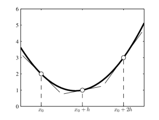
Figure 1: Numerical derivatives of a three point sequence. For the three point sequence there is a single interpolating parabola. Its tangent lines at the discrete points are shown to indicate the numerical derivatives.

This concept is extended to longer sequences of points, as shown in Figure 2. The central formula, Equation (8), is used everywhere where there are values to the left and right. The left and right end-points use Equations (7) and (9), respectively. Clearly, the first two points use the same interpolating polynomial, and similarly for the last two points.

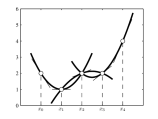
Figure 2: Numerical derivatives of a five point sequence with second order accurate formulas. There are three interpolating parabolas, whereby the first and last determine the derivatives for the end points. The indicated tangent slopes are all second order accurate.

Obviously, for long sequences of points, keeping track of such formulas will obscure the structure of the problem at hand. The algebra involved in many problems such as surface reconstruction from gradients is greatly simplified by taking a matrix algebraic approach to differentiation; specifically, we can write the three point formulas in matrix form as,

$$\begin{bmatrix}f^{\prime}\!\left(x_{0}\right)\\ f^{\prime}\!\left(x_{1}\right)\\ f^{\prime}\!\left(x_{2}\right)\end{bmatrix}\approx\frac{1}{2h}\begin{bmatrix}-3&4&-1\\ -1&0&1\\ 1&-4&3\end{bmatrix}\begin{bmatrix}f\!\left(x_{0}\right)\\ f\!\left(x_{1}\right)\\ f\!\left(x_{2}\right)\end{bmatrix}$$ (10)

Similarly, for the five point sequence shown in Figure 2, the appropriate matrix operation to compute the numerical derivatives is,

$$\begin{bmatrix}f^{\prime}\!\left(x_{0}\right)\\ f^{\prime}\!\left(x_{1}\right)\\ f^{\prime}\!\left(x_{2}\right)\\ f^{\prime}\!\left(x_{3}\right)\\ f^{\prime}\!\left(x_{4}\right)\end{bmatrix}\approx\frac{1}{2h}\begin{bmatrix}-3&4&-1&0&0\\ -1&0&1&0&0\\ 0&-1&0&1&0\\ 0&0&-1&0&1\\ 0&0&1&-4&3\end{bmatrix}\begin{bmatrix}f\!\left(x_{0}\right)\\ f\!\left(x_{1}\right)\\ f\!\left(x_{2}\right)\\ f\!\left(x_{3}\right)\\ f\!\left(x_{4}\right)\end{bmatrix}.$$ (11)

This concept of matrix based numerical differentiation is fundamental to the methods derived in this paper, since generally, the numerical differentiation of the discrete function $\boldsymbol{y}=f\left(\boldsymbol{x}\right)$ can be represented and computed by the matrix-algebraic equation,

$$\boldsymbol{y}^{\prime}=\mathsf{D}\boldsymbol{y}.$$ (12)

Under this premise, we will henceforth omit the $\approx$ under the contention that the numerical derivative is equal to this relation.
The advantage of this matrix based approach is that without difficulty, higher order derivative formulas can be used. For example, the five point formulas are

$$\begin{bmatrix}f^{\prime}\!\left(x_{0}\right)\\ f^{\prime}\!\left(x_{1}\right)\\ f^{\prime}\!\left(x_{2}\right)\\ f^{\prime}\!\left(x_{3}\right)\\ f^{\prime}\!\left(x_{4}\right)\end{bmatrix}\approx\frac{1}{12h}\begin{bmatrix}-25&48&-36&16&-3\\ -3&-10&18&-6&1\\ 1&-8&0&8&-1\\ -1&6&-18&10&3\\ 3&-16&36&-48&25\end{bmatrix}\begin{bmatrix}f\!\left(x_{0}\right)\\ f\!\left(x_{1}\right)\\ f\!\left(x_{2}\right)\\ f\!\left(x_{3}\right)\\ f\!\left(x_{4}\right)\end{bmatrix}$$ (13)

and are fourth order accurate. In contrast, methods described in the literature cannot be extended beyond the use of forward and backward differences. Besides being only first order accurate, this unfortunately leads to some inconsistencies. Specifically, for a three point sequence, both the formulas,

$$\begin{bmatrix}f^{\prime}\!\left(x_{0}\right)\\ f^{\prime}\!\left(x_{1}\right)\\ f^{\prime}\!\left(x_{2}\right)\end{bmatrix}\approx\frac{1}{h}\begin{bmatrix}-1&1&0\\ -1&1&0\\ 0&-1&1\end{bmatrix}\begin{bmatrix}f\!\left(x_{0}\right)\\ f\!\left(x_{1}\right)\\ f\!\left(x_{2}\right)\end{bmatrix}$$ (14)

and

$$\begin{bmatrix}f^{\prime}\!\left(x_{0}\right)\\ f^{\prime}\!\left(x_{1}\right)\\ f^{\prime}\!\left(x_{2}\right)\end{bmatrix}\approx\frac{1}{h}\begin{bmatrix}-1&1&0\\ 0&-1&1\\ 0&-1&1\end{bmatrix}\begin{bmatrix}f\!\left(x_{0}\right)\\ f\!\left(x_{1}\right)\\ f\!\left(x_{2}\right)\end{bmatrix}$$ (15)

are first order accurate, however, are obviously different. When working with forward and backward differences, at some point in the sequence one must switch from forward to backward in order that appropriate formulas are used at the end points. Commonly, the sequence forward/central/backward is used resulting in the operator,

$$\begin{bmatrix}f^{\prime}\!\left(x_{0}\right)\\ f^{\prime}\!\left(x_{1}\right)\\ f^{\prime}\!\left(x_{2}\right)\end{bmatrix}\approx\frac{1}{2h}\begin{bmatrix}-2&2&0\\ -1&0&1\\ 0&-2&2\end{bmatrix}\begin{bmatrix}f\!\left(x_{0}\right)\\ f\!\left(x_{1}\right)\\ f\!\left(x_{2}\right)\end{bmatrix}.$$ (16)

While these are theoretically correct derivative formulas, the are inconsistent, since the central formula is second order accurate in contrast to the forward/backward formulas which are only first order accurate. Consistency at the endpoints is all the more critical when considering boundary conditions. Unfortunately, such discussions of the end points are more often than not completely avoided in the literature (e.g., horn1986 ), and even altogether incorrect formulas are used (e.g., agrawal2006 ).
Throughout this section, for simplicity, it has been assumed that the data is on evenly spaced points. However, it is not difficult to derive the appropriate formulas for arbitrary node spacing, $h_{k}$; said formulas have been omitted for clarity.

2.2 Surface Reconstruction from Gradients

The novelty of formulating numerical differentiation as a matrix multiplication is that the partial derivatives of a surface take the particularly simple form,

$$\frac{\partial\mathsf{Z}}{\partial x} = \mathsf{Z}\mathsf{D}^{\textrm{T}}_{x}$$ (17)

$$\frac{\partial\mathsf{Z}}{\partial y} = \mathsf{D}_{y}\mathsf{Z}.$$ (18)

Note that $\mathsf{D}_{x}$ is defined as a differentiation matrix, as above, and is transposed to effect differentiation in the $x$-direction. To address the reconstruction problem, we denote a measured gradient field, obtained for example via Photometric Stereo woodham1980 , as $\mathsf{\hat{Z}}_{x}$ and $\mathsf{\hat{Z}}_{y}$. The reconstruction problem can then be formulated as finding the surface $\mathsf{Z}$ such that,

$$\mathsf{\hat{Z}}_{x}\approx\mathsf{Z}\mathsf{D}^{\textrm{T}}_{x}\quad\textrm{and}\quad\mathsf{\hat{Z}}_{y}\approx\mathsf{D}_{y}\mathsf{Z}$$ (19)

where $\approx$ denotes equality in the least-squares sense. The global least squares cost function for the reconstruction of a surface from its gradient field Harker2008c is therefore written in terms of the matrix Frobenius norm as,

$$\epsilon(\mathsf{Z})=\left\|\mathsf{Z}\mathsf{D}^{\textrm{T}}_{x}-\mathsf{\hat{Z}}_{x}\right\|_{\textrm{F}}^{2}+\left\|\mathsf{D}_{y}\mathsf{Z}-\mathsf{\hat{Z}}_{y}\right\|_{\textrm{F}}^{2},$$ (20)

which represents the Euclidean distance from the measured gradient field to the gradient field of an unknown surface $\mathsf{Z}$. From a mathematical point of view, this cost function can be considered to be a discrete functional in reference to the calculus of variations, whereby, it is a function of the unknown function (surface) $\mathsf{Z}$. To find the minimum of the cost function, we differentiate with respect to the matrix $\mathsf{Z}$, yielding the effective normal equations of the least-squares problem,

$$\mathsf{D}^{\textrm{T}}_{y}\mathsf{D}_{y}\mathsf{Z}+\mathsf{Z}\mathsf{D}^{\textrm{T}}_{x}\mathsf{D}_{x}-\mathsf{D}^{\textrm{T}}_{y}\mathsf{\hat{Z}}_{y}-\mathsf{\hat{Z}}_{x}\mathsf{D}_{x}=\mathsf{0}.$$ (21)

This matrix equation is a set of equations which are linear in the unknowns $z_{ij}$, and is known as a Sylvester Equation (cf. Equation (1) and see also Stewart2 ). Due to the fact that differentiation matrices are involved, this equation is rank-one deficient, which would normally indicate a non-unique solution bartels1972 . However, it is shown in Section 7 that the solution to this equation is unique up to a constant of integration, as expected.

2.3 Numerical Solution of Sylvester Equations

The most common approach horn1986 ; karacali2003 ; horovitz2004 ; agrawal2006 ; ng2010 ; koskulics2012 ; balzer2012 to the surface reconstruction from gradients problem proceeds by “vectorizing” the surface $\mathsf{Z}$. That is, by writing,

$$\boldsymbol{z}=\begin{bmatrix}\boldsymbol{z}_{1}\\ \vdots\\ \boldsymbol{z}_{n}\end{bmatrix},$$ (22)

where the $\boldsymbol{z}_{k}$ are a column partitioning of $\mathsf{Z}$, i.e.,

$$\mathsf{Z}=\begin{bmatrix}\boldsymbol{z}_{1}&\cdots&\boldsymbol{z}_{n}\end{bmatrix}.$$ (23)

This operation is usually denoted,

$$\boldsymbol{z}=\mathop{\mathrm{vec}}\left(\mathsf{Z}\right).$$ (24)

The resulting linear system of equations to be solved is therefore of the form,

$$\mathsf{A}\boldsymbol{z}=\boldsymbol{b},$$ (25)

where the coefficient matrix $\mathsf{A}$ is $2mn\times mn$. The relation of these commonly used methods and the approach based on the Frobenius norm approach proposed in Harker2008c can be seen by means of applying the “vec” operator to the cost function in Equation (20). The cost function in terms of the Frobenius norm is algebraically equivalent to the standard linear least squares problem,

$$\begin{bmatrix}\mathsf{D}_{x}\otimes\mathsf{I}_{m}\\ \mathsf{I}_{n}\otimes\mathsf{D}_{y}\end{bmatrix}\mathop{\mathrm{vec}}\left(\mathsf{Z}\right)=\begin{bmatrix}\mathop{\mathrm{vec}}\left(\mathsf{\hat{Z}}_{x}\right)\\ \mathop{\mathrm{vec}}\left(\mathsf{\hat{Z}}_{y}\right)\end{bmatrix}$$ (26)

where $\otimes$ denotes the Kronecker product Stewart2 . The coefficient matrix of this least squares problem is similarly $2mn\times mn$. Since the appropriate solution of this problem requires a Moore-Penrose pseudo-inverse (or its numerical equivalent), the solution in this manner is necessarily computationally intensive. The number of floating point operations to solve this if the coefficient matrix is full is,

$$W_{\textrm{VEC}}=41m^{3}n^{3},$$ (27)

and is therefore an $\mathcal{O}\!\left(n^{6}\right)$ method (cf. Higham (higham, , Ch.16)). A much more efficient manner is to work with the Sylvester Equation directly, i.e., Equation (21), as proposed in Harker2008c ; harker2011 . A common method for solving Sylvester Equations is that of Bartels and Stewart bartels1972 , and is described in Stewart2 . A generally more efficient solution is the Hessenberg-Schur method of Golub et al. golub1979 . The number of flops (floating point operations), or work required, to compute the solution using this method is,

$$W_{\textrm{HS}}\left(m,n\right)=\frac{5}{3}m^{3}+10n^{3}+5m^{2}n+\frac{5}{2}mn^{2}.$$ (28)

Clearly, the approach via the Sylvester Equation is an $\mathcal{O}\!\left(n^{3}\right)$ algorithm, in stark contrast to the vectorization approach which yields an $\mathcal{O}\!\left(n^{6}\right)$ algorithm; the significance of this difference can be seen when one considers that for most real problems $m$ and $n$ will be of the order of thousands (e.g., megapixel images from Photometric Stereo). All of the new regularization methods presented in the following are shown to fall into the Sylvester Equation framework, and therefore share in these computational advantages.

3 Spectral Regularization

3.1 Generalized Fourier Series of Discrete Orthogonal Basis Functions

A Generalized Fourier Series is the series expansion of a function in terms of a complete set of orthogonal functions, $\varphi_{k}(x)$, as,

$$f(x)=\sum_{k=0}^{\infty}\alpha_{k}\varphi_{k}(x).$$ (29)

Computation of the coefficients, $\alpha_{k}$, arises from the weighted least squares approximation of the function by the series, that is, by minimizing the function,

$$\epsilon(\alpha_{0},\ldots,\alpha_{\infty})=\int_{a}^{b}w(x)\left(f(x)-\sum_{k=0}^{\infty}\alpha_{k}\varphi_{k}(x)\right)^{2}\textrm{d}x,$$ (30)

where $w(x)$ is a positive weighting function. Differentiating with respect to the ${j}^{\textrm{th}}$ coefficient, $\alpha_{j}$ yields,

$$\frac{\partial\epsilon}{\partial\alpha_{j}}=2\int_{a}^{b}w(x)\left(f(x)-\sum_{k=0}^{\infty}\alpha_{k}\varphi_{k}(x)\right)\varphi_{j}(x)\,\textrm{d}x,$$ (31)

whereby equating to zero yields the relation,

$$\int_{a}^{b}w(x)f(x)\varphi_{j}(x)\textrm{d}x=\sum_{k=0}^{\infty}\alpha_{k}\int_{a}^{b}w(x)\varphi_{k}(x)\varphi_{j}(x)\,\textrm{d}x.$$ (32)

Thus, if the basis functions satisfy the orthogonality condition,

$$\int_{a}^{b}w(x)\varphi_{k}(x)\varphi_{j}(x)\textrm{d}x=\kappa_{k}\delta_{kj},$$ (33)

Then each of the coefficients is given as,

$$\alpha_{k}=\frac{1}{\kappa_{k}}\int_{a}^{b}w(x)f(x)\varphi_{k}(x)\,\textrm{d}x.$$ (34)

When working in the discrete domain, however, the function $f(x)$ is only known at a finite number of points, and hence the coefficients cannot be computed in this manner. To this end, we require so-called discrete orthogonal basis functions, which are continuous basis functions that are orthogonal over a discrete measure. That is to say that the orthogonality condition reads,

$$\int_{a}^{b}w(x)\varphi_{k}(x)\varphi_{j}(x)\textrm{d}\lambda(x)=\kappa_{k}\delta_{kj},$$ (35)

where the measure $\lambda(x)$ has the differential,

$$\textrm{d}\lambda(x)=\sum_{i=1}^{n}\delta(x-x_{i})\,\textrm{d}x,$$ (36)

where the $x_{i}$ are the abscissae where the value of $f(x)$ is known. Thus, by the sifting property of the delta function, the discrete orthogonality condition is,

$$\sum_{i=1}^{n}w(x_{i})\varphi_{k}(x_{i})\varphi_{j}(x_{i})=\kappa_{k}\delta_{kj}.$$ (37)

The coefficients for the discrete Generalized Fourier Series are then given as,

$$\alpha_{k}=\frac{1}{\kappa_{k}}\sum_{i=1}^{n}w(x_{i})f(x_{i})\varphi(x_{i}),$$ (38)

which clearly only requires the values of the function $f(x)$ at the ordered set of nodes $x_{k}$, $k=1,\ldots,n$. Discrete basis functions were originally created as a computationally efficient solution to the interpolation–approximation problem (e.g., the Gram polynomials gram1883 ). To compute the coefficients of a discrete series, we also only require the values of the basis functions at the set of nodes, which can be conveniently arranged and manipulated in matrix form as,

$$\mathsf{B}=\begin{bmatrix}\varphi_{0}(x_{1})&\varphi_{1}(x_{1})&\cdots&\varphi_{n-1}(x_{1})\\ \varphi_{0}(x_{2})&\varphi_{1}(x_{2})&\cdots&\varphi_{n-1}(x_{2})\\ \vdots&\vdots&\ddots&\vdots\\ \varphi_{0}(x_{n})&\varphi_{1}(x_{n})&\cdots&\varphi_{n-1}(x_{n})\\ \end{bmatrix}$$ (39)

In this manner, the function $\boldsymbol{y}=f\!\left(\boldsymbol{x}\right)$ is then described as

$$\boldsymbol{y}=\mathsf{B}\boldsymbol{\alpha}$$ (40)

whereby the matrix $\mathsf{B}$ can be viewed as composed column-wise of vector basis functions,

$$\mathsf{B}=\begin{bmatrix}\boldsymbol{b}_{0}(\boldsymbol{x})&\boldsymbol{b}_{1}(\boldsymbol{x})&\cdots&\boldsymbol{b}_{n-1}(\boldsymbol{x})\end{bmatrix}$$ (41)

and satisfies the orthogonality condition,

$$\mathsf{B}^{\textrm{T}}\mathsf{W}\mathsf{B}=\mathsf{I},$$ (42)

usually with the added condition that the weighting matrix, $\mathsf{W}$, is positive definite. Clearly when working with discrete basis functions, the series expansion of a function is necessarily finite. Further, any function (vector) can be represented by such a series provided that the set of basis functions is complete; the completeness of the set of basis functions, $\boldsymbol{b}_{k}$, entails that the matrix $\mathsf{B}$ is $n\times n$ and full rank. To extend discrete orthogonal basis functions to a 2D domain, we define the basis functions $\mathsf{B}_{x}$ and $\mathsf{B}_{y}$ respectively for the $x$ and $y$ directions. The surface $\mathsf{Z}$ is then represented as,

$$\mathsf{Z}=\mathsf{B}_{y}\mathsf{C}\mathsf{B}^{\textrm{T}}_{x},$$ (43)

where the matrix $\mathsf{C}$ represents the generalized Fourier coefficients. If the basis functions satisfy the orthogonality conditions,

$$\mathsf{B}^{\textrm{T}}_{x}\mathsf{W}_{x}\mathsf{B}_{x} = \mathsf{I}_{n}$$ (44)

$$\mathsf{B}^{\textrm{T}}_{y}\mathsf{W}_{y}\mathsf{B}_{y} = \mathsf{I}_{m}$$ (45)

then the minimizing coefficients of the weighted least squares cost function (weighted Frobenius norm),

$$\epsilon(\mathsf{C})=\left\|\mathsf{W}_{y}^{\frac{1}{2}}\left(\mathsf{Z}-\mathsf{B}_{y}\mathsf{C}\mathsf{B}^{\textrm{T}}_{x}\right)\mathsf{W}_{x}^{\frac{1}{2}}\right\|_{\textrm{F}}^{2}$$ (46)

are the generalized Fourier coefficients,

$$\mathsf{C}=\mathsf{B}^{\textrm{T}}_{y}\mathsf{W}_{y}\mathsf{Z}\mathsf{W}_{x}\mathsf{B}_{x}$$ (47)

Some examples of functions which can be considered to be generalized Fourier series in the discrete sense are Gram Polynomials oleary2008b , Cosine/Sine Functions (e.g. DCT), Fourier Basis Functions, Haar Functions haar1910 , Hartley Transform Basis Functions bracewell , etc.

3.2 Surface Reconstruction with GFS

According to Equation (47) we can represent a reconstructed surface exactly with any complete set of basis functions. Hence using the complete set of basis functions should have no influence on the surface reconstruction other than to increase the computational load. On the other hand, if we use an incomplete (or truncated) set of basis functions, then we can effectively incorporate band-pass filtering into the least squares solution. Specifically, we represent $\mathsf{Z}$ as the truncated generalized Fourier series,

$$\mathsf{Z}=\mathsf{B}_{y}\mathsf{C}\mathsf{B}^{\textrm{T}}_{x},$$ (48)

where $\mathsf{B}_{y}$ is a set of $p$ basis functions on $m$ nodes with $p<m$, matrix $\mathsf{B}_{x}$ is a set of $q$ basis functions on $n$ nodes with $q<n$, and the matrix $\mathsf{C}$ is a $p\times q$ matrix of generalized Fourier coefficients. For simplicity, we assume the functions are orthogonal with respect to an identity weighting, that is, the basis functions are orthonormal (The weighted least squares solution is postponed until Section 6). Thus the least squares cost function is obtained by substituting the surface representation in Equation (48) into Equation (20), i.e.,

$$\epsilon(\mathsf{C})=\left\|\mathsf{B}_{y}\mathsf{C}\mathsf{B}^{\textrm{T}}_{x}\mathsf{D}^{\textrm{T}}_{x}-\mathsf{\hat{Z}}_{x}\right\|_{\textrm{F}}^{2}+\left\|\mathsf{D}_{y}\mathsf{B}_{y}\mathsf{C}\mathsf{B}^{\textrm{T}}_{x}-\mathsf{\hat{Z}}_{y}\right\|_{\textrm{F}}^{2}$$ (49)

Differentiating with respect to the unknown coefficients, $\mathsf{C}$, yields the effective normal equations,

$$\mathsf{B}^{\textrm{T}}_{y}\mathsf{D}^{\textrm{T}}_{y}\mathsf{D}_{y}\mathsf{B}_{y}\mathsf{C} + \mathsf{C}\mathsf{B}^{\textrm{T}}_{x}\mathsf{D}^{\textrm{T}}_{x}\mathsf{D}_{x}\mathsf{B}_{x}$$ (50)

$$- \mathsf{B}^{\textrm{T}}_{y}\left(\mathsf{D}^{\textrm{T}}_{y}\mathsf{\hat{Z}}_{y}+\mathsf{\hat{Z}}_{x}\mathsf{D}_{x}\right)\mathsf{B}_{x}=\mathsf{0},$$

which is a $p\times q$ Sylvester Equation in the unknown coefficients $\mathsf{C}$. Since a surface defined as a function of its spectral coefficients has, per definition, an integrable gradient field, its gradient field spans a subspace of all integrable gradient fields. That is, its gradient spans a band limited subspace of the integrable gradient fields.

3.3 Computational Aspects

The solution of the surface reconstruction problem is obtained by solving the Sylvester Equation (50) and back-substitution of the coefficients into Equation (48). Using the method of Golub et al. golub1979 , the computational work required is given by Equation (28); however, in the case of Spectral Regularization the solution of the Sylvester Equation is more efficient since an $m\times n$ equation is reduced to a $p\times q$ equation. That is, if $p$ and $q$ are some fraction of $m$ and $n$ of the form

$$p=\frac{m}{2^{k}}\qquad\textrm{and}\qquad q=\frac{n}{2^{k}},$$ (51)

then the number of flops to solve the corresponding Sylvester Equation is,

$$W\left(p,q\right)=\frac{1}{2^{3k}}W\left(m,n\right)$$ (52)

Hence, by using only half of the basis functions $(k=1)$, the work is reduced to $\frac{1}{8}$ of the full problem. By using one quarter of the basis functions $(k=2)$, the work is reduced to $\frac{1}{64}$, etc.

4 Tikhonov Regularization

Tikhonov regularization Engl over a 1D domain amounts to finding the function $\boldsymbol{y}$ which minimizes the functional,

$$\epsilon\left(\boldsymbol{y}\right)=\left\|\mathsf{A}\boldsymbol{y}-\boldsymbol{b}\right\|_{2}^{2}+\lambda^{2}\left\|\mathsf{L}\left(\boldsymbol{y}-\boldsymbol{y}_{0}\right)\right\|_{2}^{2}.$$ (53)

Whereas the former term is a typical least-squares cost function, the latter acts as a “penalty” term. The function $\boldsymbol{y}_{0}$ is an a priori estimate of the unknown function; if nothing is known about the function, then $\boldsymbol{y}_{0}$ is the zero vector. Hence the penalty term is a (weighted) measure of the deviation from the a priori estimate. Thus if $\mathsf{L}=\mathsf{I}$, then the penalty term is the Euclidean deviation of the solution from the a priori estimate. The constant $\lambda$ is the regularization parameter, which is positive and is assumed to be fixed for the optimization process; it essentially shifts the priority between the least squares residual and the regularization term. To find the minimum of the functional, it is differentiated with respect to $\boldsymbol{y}$, where upon rearranging yields,

$$\left(\mathsf{A}^{\textrm{T}}\mathsf{A}+\lambda^{2}\mathsf{L}^{\textrm{T}}\mathsf{L}\right)\boldsymbol{y}=\mathsf{A}^{\textrm{T}}\boldsymbol{b}+\lambda^{2}\mathsf{L}^{\textrm{T}}\mathsf{L}\boldsymbol{y}_{0},$$ (54)

which are the corresponding normal equations. Equation (54) is a necessary, but not sufficient, condition that $\boldsymbol{y}$ is a constrained minimizer of the least-squares cost function. For this reason, regularization is typically associated with Lagrange Multipliers; however, it is actually much more closely related to the Levenberg-Marquardt algorithm Marquardt1963 ; specifically, each step of the Levenberg-Marquardt algorithm is a Tikhonov-regularized Gauss-Newton step. For a fixed $\lambda$ the minimizing solution can be computed directly via the Moore-Penrose pseudo-inverse. The Tikhonov regularization problem is said to be in standard form if the smoothing operator $\mathsf{L}=\mathsf{I}$ and $\boldsymbol{y}_{0}=\boldsymbol{0}$.

4.1 Tikhonov Regularization for the Reconstruction Problem

For the problem of surface reconstruction from gradients, the functional to be minimized depends on a 2D surface, as opposed to a vector; hence, the common approach to Tikhonov regularization does not apply directly. To derive the appropriate functional for a 2D domain, we begin with the least squares cost function of Equation (20). We define the matrices $\mathsf{L}_{x}$ and $\mathsf{L}_{y}$ as general “smoothing” operators in the $x$- and $y$-directions, respectively; thus, the functional for Tikhonov regularization in its most general form reads,

$$\epsilon\left(\mathsf{Z}\right) = \left\|\mathsf{D}_{y}\mathsf{Z}-\mathsf{\hat{Z}}_{y}\right\|_{\textrm{F}}^{2}+\left\|\mathsf{Z}\mathsf{D}^{\textrm{T}}_{x}-\mathsf{\hat{Z}}_{x}\right\|_{\textrm{F}}^{2}$$ (55)

$$+ \mu^{2}\left\|\mathsf{L}_{y}\left(\mathsf{Z}-\mathsf{Z}_{0}\right)\right\|_{\textrm{F}}^{2}+\lambda^{2}\left\|\left(\mathsf{Z}-\mathsf{Z}_{0}\right)\mathsf{L}_{x}^{\textrm{T}}\right\|_{\textrm{F}}^{2}.$$

where $\mathsf{Z}_{0}$ is an a-priori estimate of the surface. The estimate $\mathsf{Z}_{0}$ is not necessary, since we may assume the surface is nearly flat, i.e., $\mathsf{Z}_{0}=\mathsf{0}$. However, the fact that we can incorporate this a priori estimate into the algorithm may have substantial consequences for applied Photometric Stereo. For the sake of generality, we have introduced a second regularization parameter, $\mu$, which may be of use if the $x$- and $y$-derivatives have different noise properties. Differentiating the cost function with respect to $\mathsf{Z}$ yields the corresponding normal equations of this functional, i.e.,

$$\left(\mathsf{D}^{\textrm{T}}_{y}\mathsf{D}_{y}+\mu^{2}\mathsf{L}^{\textrm{T}}_{y}\mathsf{L}_{y}\right)\mathsf{Z} + \mathsf{Z}\left(\mathsf{D}^{\textrm{T}}_{x}\mathsf{D}_{x}+\lambda^{2}\mathsf{L}^{\textrm{T}}_{x}\mathsf{L}_{x}\right)$$ (56)

$$- \mathsf{D}^{\textrm{T}}_{y}\mathsf{\hat{Z}}_{y}-\mathsf{\hat{Z}}_{x}\mathsf{D}_{x}$$

$$- \mu^{2}\mathsf{L}^{\textrm{T}}_{y}\mathsf{L}_{y}\mathsf{Z}_{0}$$

$$- \mathsf{Z}_{0}\left(\lambda^{2}\mathsf{L}^{\textrm{T}}_{x}\mathsf{L}_{x}\right)=\mathsf{0}.$$

This is again a Sylvester Equation in the unknown surface $\mathsf{Z}$. For the surface reconstruction problem, the standard form of the Tikhonov regularization problem corresponds to $\mathsf{L}_{x}=\mathsf{I}_{n}$, $\mathsf{L}_{y}=\mathsf{I}_{m}$, and $\mathsf{Z}_{0}=\mathsf{0}$, in which case it suffices to consider only $\mu=\lambda$.

4.2 Regularization Terms

In the context of a 2D reconstruction problem, the following regularization terms were derived in their matrix form in harker2011 . For completeness, the results are merely summarized here. The most basic regularization term is a bound on the norm of the solution, in this case,

$$\rho\left(\mathsf{Z}\right)=\left\|\mathsf{Z}\right\|_{\textrm{F}}^{2},$$ (57)

which is effectively a degree-0 regularization term, and corresponds to the Tikhonov problem in its standard form. It is written equivalently as,

$$\rho\left(\mathsf{Z}\right)=\frac{1}{2}\left(\left\|\mathsf{I}_{m}\mathsf{Z}\right\|_{\textrm{F}}^{2}+\left\|\mathsf{Z}\mathsf{I}_{n}\right\|_{\textrm{F}}^{2}\right),$$ (58)

such that it corresponds to the Sylvester Equation (56). A degree-1 regularization term bounds the magnitude of the maximum directional derivative, or the overall steepness of the reconstructed surface, i.e.,

$$\rho\left(\mathsf{Z}\right)=\left\|\mathsf{D}_{y}\mathsf{Z}\right\|_{\textrm{F}}^{2}+\left\|\mathsf{Z}\mathsf{D}^{\textrm{T}}_{x}\right\|_{\textrm{F}}^{2}.$$ (59)

Finally, the regularization term,

$$\rho\left(\mathsf{Z}\right)=\left\|\mathsf{D}_{y}^{2}\mathsf{Z}\right\|_{\textrm{F}}^{2}+\left\|\mathsf{Z}\left(\mathsf{D}_{x}^{2}\right)^{\textrm{T}}\right\|_{\textrm{F}}^{2},$$ (60)

is a degree-2 regularization term, and bounds the mean curvature of the surface.

4.3 Influence of the Regularization Parameter

To derive an effective algorithm for determining the regularization parameter, as well as to characterize the effect of the regularization parameter on the solution, we look at the Tikhonov problem in its standard form. Firstly, we denote the SVDs of the $x$- and $y$-derivative operators as

$$\mathsf{D}_{x} = \mathsf{U}_{x}\mathsf{S}_{x}\mathsf{V}^{\textrm{T}}_{x}=\sum_{i=1}^{n}\alpha_{i}\boldsymbol{u}_{i}\boldsymbol{v}^{\textrm{T}}_{i}$$ (61)

$$\mathsf{D}_{y} = \mathsf{U}_{y}\mathsf{S}_{y}\mathsf{V}^{\textrm{T}}_{y}=\sum_{j=1}^{m}\beta_{j}\boldsymbol{m}_{j}\boldsymbol{w}^{\textrm{T}}_{j}$$ (62)

By substitution of these relations, the normal equations for Tikhonov regularization in standard form can be written as,

$$\left(\mathsf{V}_{y}\mathsf{S}_{y}^{2}\mathsf{V}^{\textrm{T}}_{y}+\lambda^{2}\mathsf{I}_{m}\right)\mathsf{Z} + \mathsf{Z}\left(\mathsf{V}_{x}\mathsf{S}_{x}^{2}\mathsf{V}^{\textrm{T}}_{x}+\lambda^{2}\mathsf{I}_{n}\right)$$

$$-\mathsf{V}_{y}\mathsf{S}_{y}\mathsf{U}^{\textrm{T}}_{y}\mathsf{\hat{Z}}_{y} - \mathsf{\hat{Z}}_{x}\mathsf{U}_{x}\mathsf{S}_{x}\mathsf{V}^{\textrm{T}}_{x}=\mathsf{0}.$$ (63)

Pre-multiplying by $\mathsf{V}^{\textrm{T}}_{y}$ and post-multiplying by $\mathsf{V}_{x}$ yields,

$$\left(\mathsf{S}_{y}^{2}\mathsf{V}^{\textrm{T}}_{y}+\lambda^{2}\mathsf{V}^{\textrm{T}}_{y}\right)\mathsf{Z}\mathsf{V}_{x} + \mathsf{V}^{\textrm{T}}_{y}\mathsf{Z}\left(\mathsf{V}_{x}\mathsf{S}_{x}^{2}+\lambda^{2}\mathsf{V}_{x}\right)$$

$$-\mathsf{S}_{y}\mathsf{U}^{\textrm{T}}_{y}\mathsf{\hat{Z}}_{y}\mathsf{V}_{x} - \mathsf{V}^{\textrm{T}}_{y}\mathsf{\hat{Z}}_{x}\mathsf{U}_{x}\mathsf{S}_{x}=\mathsf{0}.$$ (64)

If we make the following substitution,

$$\mathsf{M}=\mathsf{V}^{\textrm{T}}_{y}\mathsf{Z}\mathsf{V}_{x},$$ (65)

then the matrix $\mathsf{M}$ represents the generalized Fourier Series coefficients of the surface $\mathsf{Z}$ with respect to the singular vectors $\mathsf{V}_{x}$ and $\mathsf{V}_{y}$. Making the further substitutions,

$$\mathsf{P} = \mathsf{U}^{\textrm{T}}_{y}\mathsf{\hat{Z}}_{y}\mathsf{V}_{x}$$ (66)

$$\mathsf{Q} = \mathsf{V}^{\textrm{T}}_{y}\mathsf{\hat{Z}}_{x}\mathsf{U}_{x}$$ (67)

then the normal equations read,

$$\left(\mathsf{S}_{y}^{2}+\lambda^{2}\mathsf{I}_{m}\right)\mathsf{M}+\mathsf{M}\left(\mathsf{S}_{x}^{2}+\lambda^{2}\mathsf{I}_{n}\right)-\mathsf{S}_{y}\mathsf{P}-\mathsf{Q}\mathsf{S}_{x}=\mathsf{0}.$$ (68)

Since all the pertinent coefficient matrices are diagonal, this equation, taken element-wise, reads,

$$\left(\beta_{i}^{2}+\lambda^{2}\right)m_{ij}+m_{ij}\left(\alpha_{j}^{2}+\lambda^{2}\right)-\beta_{i}p_{ij}-\alpha_{j}q_{ij}=0,$$ (69)

for each $i=1,\ldots,m$, $j=1,\ldots,n$. Thus, the entries of $\mathsf{M}$ can be solved for as a function of $\lambda$ as,

$$m_{ij}\left(\lambda\right)=\frac{\beta_{i}p_{ij}+\alpha_{j}q_{ij}}{\alpha_{j}^{2}+\beta_{i}^{2}+2\lambda^{2}}$$ (70)

which determines the coefficients in terms of $\lambda$. To demonstrate the influence of the regularization parameter, $\lambda$, this relation can be rewritten in the form,

$$m_{ij}\left(\lambda\right)=f_{ij}\left(\lambda\right)\frac{\beta_{i}p_{ij}+\alpha_{j}q_{ij}}{\alpha_{j}^{2}+\beta_{i}^{2}}$$ (71)

where the terms

$$f_{ij}\left(\lambda\right)=\frac{\alpha_{j}^{2}+\beta_{i}^{2}}{\alpha_{j}^{2}+\beta_{i}^{2}+2\lambda^{2}}$$ (72)

can be considered to be filter factors hansen1993 , which range from $1$ to $0$ (corresponding respectively to $\lambda=0$ and $\lambda\rightarrow\infty$). Clearly, when the filter factors are all one (i.e., $f_{ij}(0)=1$), Equation (71) represents the least-squares solution (GLS) to the reconstruction problem. The values,

$$\mu_{ij}^{2}=\alpha_{j}^{2}+\beta_{i}^{2},$$ (73)

are the eigenvalues of the Sylvester Operator Stewart2 , and thus writing the filter factors as,

$$f_{ij}\left(\lambda\right)=\frac{\mu_{ij}^{2}}{\mu_{ij}^{2}+2\lambda^{2}},$$ (74)

shows that Tikhonov regularization for the reconstruction problem in Sylvester Equation form, has essentially the same structure as standard 1-dimensional domain Tikhonov regularization problems, cf. hansen1993 . As can be seen from the filter factors, the regularization parameter $\lambda$ inversely weights the coefficients $m_{ij}$. This influence of $\lambda$ on the reconstructed surface can be seen from Equation (65), since the reconstructed surface can be written as,

$$\mathsf{Z}\left(\lambda\right)=\sum_{i=1}^{m}\sum_{j=1}^{n}m_{ij}\left(\lambda\right)\boldsymbol{w}_{i}\boldsymbol{v}^{\textrm{T}}_{j},$$ (75)

The reconstructed surface is therefore sum of rank-1 matrices each weighted by the coefficients $m_{ij}$, which are functions of the regularization parameter $\lambda$. Clearly, the parameter $\lambda$ has a larger influence on basis functions corresponding to small singular values; specifically, basis functions associated with small singular values are largely suppressed. Note that this analysis constitutes an algorithm for solving symmetric rank-deficient Sylvester Equations; however, here it is used as a means of effectively determining the regularization parameter $\lambda$.

4.4 Selection of the Regularization Parameter

The L-curve is a plot of $\left(\rho\left(\lambda\right),\eta\left(\lambda\right)\right)$ where, $\rho^{2}\left(\lambda\right)$ is the least-squares cost function,

$$\rho^{2}\left(\lambda\right)=\left\|\mathsf{Z}\left(\lambda\right)\mathsf{D}^{\textrm{T}}_{x}-\mathsf{\hat{Z}}_{x}\right\|_{\textrm{F}}^{2}+\left\|\mathsf{D}_{y}\mathsf{Z}\left(\lambda\right)-\mathsf{\hat{Z}}_{y}\right\|_{\textrm{F}}^{2}$$ (76)

and $\eta^{2}\left(\lambda\right)$ is the regularization term (in standard form),

$$\eta^{2}\left(\lambda\right)=\left\|\mathsf{Z}\left(\lambda\right)\right\|_{\textrm{F}}^{2}$$ (77)

Thus, the L-curve is a visualization of the interplay of the least squares residual, and the magnitude of the regularization term. Once the singular value decompositions of the derivative matrices are computed, points on the L-curve can be computed as,

$$\rho^{2}\left(\lambda\right)=\left\|\mathsf{M}\left(\lambda\right)\mathsf{S}_{x}-\mathsf{Q}\right\|_{\textrm{F}}^{2}+\left\|\mathsf{S}_{y}\mathsf{M}\left(\lambda\right)-\mathsf{P}\right\|_{\textrm{F}}^{2}$$ (78)

and

$$\eta^{2}\left(\lambda\right)=\left\|\mathsf{M}\left(\lambda\right)\right\|_{\textrm{F}}^{2}$$ (79)

due to the invariance of the Frobenius norm under orthonormal transformation. The computational cost of these evaluations are relatively small in comparison to the computation of the singular value decomposition, due to the fact that $\mathsf{S}_{x}$ and $\mathsf{S}_{y}$ are diagonal. The result is that several points on the L-curve can be computed to determine an appropriate regularization parameter. Further analysis of regularization parameter selection is beyond the scope of this paper; the reader is referred to Engl ; GolubMeurant .

5 Constraining Solutions by Known Boundary Conditions

Boundary conditions are usually imposed as auxiliary conditions to partial differential equations to ensure the existence of a unique solution. For the surface reconstruction from gradients problem, they can be imposed to constrain the solution, which effects a form of regularization on the reconstructed surface. Dirichlet Boundary Conditions specify the value of the integral surface on the domain boundary, and can have highly effective regularizing effects (See Section 8). Neumann Boundary Conditions specify the value of the normal derivative of the integral surface on the domain boundary, and hence has a similar effect to first order Tikhonov Regularization. In the following, we derive the solution to the reconstruction problem with arbitrary Dirichlet Conditions.

5.1 Dirichlet Boundary Conditions

Dirichlet boundary conditions specify the value of the function (in this case the height of the surface) on the boundary of the domain. Using a matrix based approach, we start by parameterizing a surface with fixed height on the boundary. This can be accomplished with permutation matrices; specifically,

$$\mathsf{Z}=\mathsf{P}_{m}\mathsf{Z}_{\textrm{I}}\mathsf{P}^{\textrm{T}}_{n}+\mathsf{Z}_{\textrm{B}},$$ (80)

where $\mathsf{P}_{m}$ and $\mathsf{P}_{n}$ are the (orthonormal) permutation matrices,

$$\mathsf{P}_{m}=\begin{bmatrix}\boldsymbol{0}^{\textrm{T}}\\ \mathsf{I}_{m-2}\\ \boldsymbol{0}^{\textrm{T}}\end{bmatrix}\qquad\textrm{and}\qquad\mathsf{P}_{n}=\begin{bmatrix}\boldsymbol{0}^{\textrm{T}}\\ \mathsf{I}_{n-2}\\ \boldsymbol{0}^{\textrm{T}}\end{bmatrix}.$$ (81)

The matrix $\mathsf{Z}_{\textrm{I}}$ is the $\left(m-2\right)\times\left(n-2\right)$ matrix of the unknown interior values of the surface and $\mathsf{Z}_{\textrm{B}}$ is the $m\times n$ matrix specifying the boundary values. Substituting this parametrization into the cost function for the surface reconstruction problem, i.e., Equation (20), yields,

$$\epsilon(\mathsf{Z}_{\textrm{I}}) = \left\|\left(\mathsf{P}_{m}\mathsf{Z}_{\textrm{I}}\mathsf{P}^{\textrm{T}}_{n}+\mathsf{Z}_{\textrm{B}}\right)\mathsf{D}^{\textrm{T}}_{x}-\mathsf{\hat{Z}}_{x}\right\|_{\textrm{F}}^{2}$$ (82)

$$+ \left\|\mathsf{D}_{y}\left(\mathsf{P}_{m}\mathsf{Z}_{\textrm{I}}\mathsf{P}^{\textrm{T}}_{n}+\mathsf{Z}_{\textrm{B}}\right)-\mathsf{\hat{Z}}_{y}\right\|_{\textrm{F}}^{2}$$

Differentiating the functional with respect to $\mathsf{Z}_{\textrm{I}}$ yields the effective normal equations,

$$\mathsf{P}^{\textrm{T}}_{m}\mathsf{D}^{\textrm{T}}_{y}\mathsf{D}_{y}\mathsf{P}_{m}\mathsf{Z}_{\textrm{I}} + \mathsf{Z}_{\textrm{I}}\mathsf{P}^{\textrm{T}}_{n}\mathsf{D}^{\textrm{T}}_{x}\mathsf{D}_{x}\mathsf{P}_{n}$$ (83)

$$- \mathsf{P}^{\textrm{T}}_{m}\left(\mathsf{\hat{Z}}_{x}-\mathsf{Z}_{\textrm{B}}\mathsf{D}^{\textrm{T}}_{x}\right)\mathsf{D}_{x}\mathsf{P}_{n}$$

$$- \mathsf{P}^{\textrm{T}}_{m}\mathsf{D}^{\textrm{T}}_{y}\left(\mathsf{\hat{Z}}_{y}-\mathsf{D}_{y}\mathsf{Z}_{\textrm{B}}\right)\mathsf{P}_{n}=\mathsf{0},$$

which is an $\left(m-2\right)\times\left(n-2\right)$ Sylvester Equation in the unknown interior portion of the surface $\mathsf{Z}_{\textrm{I}}$.

6 Weighted Least Squares Solutions

Weighted least squares is an important extension of the standard least squares problem when measurement errors behave according to heteroscedastic Gaussian distributions. The maximum likelihood cost function is the standard least squares cost function modified by the inverse square root of the covariance matrix of the errors in measuring $\boldsymbol{b}$, i.e.,

$$\boldsymbol{y}_{\textrm{M}}=\min_{\boldsymbol{y}}\left\|\mathsf{\Lambda}^{-\frac{1}{2}}\left(\mathsf{A}\boldsymbol{y}-\boldsymbol{b}\right)\right\|_{2}^{2}$$ (84)

This cost function corresponds to the Mahalanobis distance between $\mathsf{A}\boldsymbol{y}$ and $\boldsymbol{b}$, whereby, minimization proceeds by differentiating with respect to $\boldsymbol{y}$ and solving the corresponding normal equations.

6.1 Mahalanobis Distance between two Gradient Fields

If we assume that the errors in measuring a gradient field are non-uniform and covariant, then the measured gradient field is related to the true gradient field by,

$$\mathsf{\hat{Z}}_{x} = \mathsf{Z}_{x}+\mathsf{\Lambda}_{xy}^{\frac{1}{2}}\mathsf{\Delta}_{x}\mathsf{\Lambda}_{xx}^{\frac{1}{2}}$$ (85)

$$\mathsf{\hat{Z}}_{y} = \mathsf{Z}_{y}+\mathsf{\Lambda}_{yy}^{\frac{1}{2}}\mathsf{\Delta}_{y}\mathsf{\Lambda}_{yx}^{\frac{1}{2}}$$ (86)

where $\mathsf{\Delta}_{x}$ and $\mathsf{\Delta}_{y}$ are matrices of i.i.d. Gaussian random variables; the covariance matrices, $\mathsf{\Lambda}_{uv}$, denote the covariance of the $u$-derivative in the $v$-direction, and for simplicity the matrix square root is specifically its symmetric square root. In this case, the measured gradient is related to the true gradient in terms of the Mahalanobis distance. The minimum Mahalanobis distance is then characterized by the least squares minimization of the term,

$$\left\|\mathsf{\Delta}_{x}\right\|_{\textrm{F}}^{2}+\left\|\mathsf{\Delta}_{y}\right\|_{\textrm{F}}^{2}$$ (87)

Therefore, the Mahalanobis distance between two gradient fields is given as,

$$\epsilon_{\textrm{M}} = \left\|\mathsf{\Lambda}_{xy}^{-\frac{1}{2}}\left(\mathsf{Z}_{x}-\mathsf{\hat{Z}}_{x}\right)\mathsf{\Lambda}_{xx}^{-\frac{1}{2}}\right\|_{\textrm{F}}^{2}$$ (88)

$$+ \left\|\mathsf{\Lambda}_{yy}^{-\frac{1}{2}}\left(\mathsf{Z}_{y}-\mathsf{\hat{Z}}_{y}\right)\mathsf{\Lambda}_{yx}^{-\frac{1}{2}}\right\|_{\textrm{F}}^{2}$$

which can be considered to be a weighted Frobenius norm, as proposed in higham2002 .

6.2 Weighted Solution for Surface Reconstruction

Given the expression for the Mahalanobis between two gradient fields, the weighted least squares surface reconstruction from gradients can be posed as the minimization of the functional,

$$\epsilon\left(\mathsf{Z}\right) = \left\|\mathsf{\Lambda}_{xy}^{-\frac{1}{2}}\left(\mathsf{Z}\mathsf{D}^{\textrm{T}}_{x}-\mathsf{\hat{Z}}_{x}\right)\mathsf{\Lambda}_{xx}^{-\frac{1}{2}}\right\|_{\textrm{F}}^{2}$$ (89)

$$+ \left\|\mathsf{\Lambda}_{yy}^{-\frac{1}{2}}\left(\mathsf{D}_{y}\mathsf{Z}-\mathsf{\hat{Z}}_{y}\right)\mathsf{\Lambda}_{yx}^{-\frac{1}{2}}\right\|_{\textrm{F}}^{2}$$

Differentiating the functional with respect to $\mathsf{Z}$ yields the effective normal equations, i.e.,

$$\mathsf{D}^{\textrm{T}}_{y}\mathsf{\Lambda}_{yy}^{-1}\mathsf{D}_{y}\mathsf{Z}\mathsf{\Lambda}_{yx}^{-1} + \mathsf{\Lambda}_{xy}^{-1}\mathsf{Z}\mathsf{D}^{\textrm{T}}_{x}\mathsf{\Lambda}_{xx}^{-1}\mathsf{D}_{x}$$

$$- \mathsf{D}^{\textrm{T}}_{y}\mathsf{\Lambda}_{yy}^{-1}\mathsf{\hat{Z}}_{y}\mathsf{\Lambda}_{yx}^{-1}-\mathsf{\Lambda}_{xy}^{-1}\mathsf{\hat{Z}}_{x}\mathsf{\Lambda}_{xx}^{-1}\mathsf{D}_{x}=\mathsf{0},$$

which is not immediately a Sylvester Equation. However, by pre-multiplying by $\mathsf{\Lambda}_{xy}^{\frac{1}{2}}$, post-multiplying by $\mathsf{\Lambda}_{yx}^{\frac{1}{2}}$, and inserting the expressions,

$$\mathsf{\Lambda}_{xy}^{\frac{1}{2}}\mathsf{\Lambda}_{xy}^{-\frac{1}{2}}=\mathsf{I}\qquad\textrm{and}\qquad\mathsf{\Lambda}_{yx}^{-\frac{1}{2}}\mathsf{\Lambda}_{yx}^{\frac{1}{2}}=\mathsf{I},$$ (91)

we yield the symmetric form,

$$\left(\mathsf{\Lambda}_{xy}^{\frac{1}{2}}\mathsf{D}^{\textrm{T}}_{y}\mathsf{\Lambda}_{yy}^{-1}\mathsf{D}_{y}\mathsf{\Lambda}_{xy}^{\frac{1}{2}}\right)\mathsf{Z}_{\textrm{w}} + \mathsf{Z}_{\textrm{w}}\left(\mathsf{\Lambda}_{yx}^{\frac{1}{2}}\mathsf{D}^{\textrm{T}}_{x}\mathsf{\Lambda}_{xx}^{-1}\mathsf{D}_{x}\mathsf{\Lambda}_{yx}^{\frac{1}{2}}\right)$$

$$- \mathsf{\Lambda}_{xy}^{\frac{1}{2}}\mathsf{D}^{\textrm{T}}_{y}\mathsf{\Lambda}_{yy}^{-1}\mathsf{\hat{Z}}_{y}\mathsf{\Lambda}_{yx}^{-\frac{1}{2}}$$

$$- \mathsf{\Lambda}_{xy}^{-\frac{1}{2}}\mathsf{\hat{Z}}_{x}\mathsf{\Lambda}_{xx}^{-1}\mathsf{D}_{x}\mathsf{\Lambda}_{xy}^{\frac{1}{2}}=\mathsf{0}$$

which is a Sylvester Equation in the unknown “weighted” surface $\mathsf{Z}_{\textrm{w}}$, where,

$$\mathsf{Z}_{\textrm{w}}=\mathsf{\Lambda}_{xy}^{-\frac{1}{2}}\mathsf{Z}\mathsf{\Lambda}_{yx}^{-\frac{1}{2}}.$$ (93)

The weighted Sylvester Equation in Equation (6.2) can be clarified with some simplified notation, i.e., it can be written in the form,

$$\mathsf{A}^{\textrm{T}}\mathsf{A}\mathsf{Z}_{\textrm{w}}+\mathsf{Z}_{\textrm{w}}\mathsf{B}^{\textrm{T}}\mathsf{B}-\mathsf{A}^{\textrm{T}}\mathsf{F}-\mathsf{G}\mathsf{B}=\mathsf{0}$$ (94)

where $\mathsf{A}$ and $\mathsf{B}$ can be considered to be weighted differential operators,

$$\mathsf{A} = \mathsf{\Lambda}_{yy}^{-\frac{1}{2}}\mathsf{D}_{y}\mathsf{\Lambda}_{xy}^{\frac{1}{2}}$$ (95)

$$\mathsf{B} = \mathsf{\Lambda}_{xx}^{-\frac{1}{2}}\mathsf{D}_{x}\mathsf{\Lambda}_{yx}^{\frac{1}{2}}$$ (96)

and $\mathsf{F}$ and $\mathsf{G}$ can be considered to be the weighted gradient field,

$$\mathsf{F} = \mathsf{\Lambda}_{yy}^{-\frac{1}{2}}\mathsf{\hat{Z}}_{y}\mathsf{\Lambda}_{yx}^{-\frac{1}{2}}$$ (97)

$$\mathsf{G} = \mathsf{\Lambda}_{xy}^{-\frac{1}{2}}\mathsf{\hat{Z}}_{x}\mathsf{\Lambda}_{xx}^{-\frac{1}{2}}$$ (98)

Upon solving Equation (6.2), or equivalently, Equation (94), for $\mathsf{Z}_{\textrm{w}}$ the weighted least squares solution is obtained as,

$$\mathsf{Z}=\mathsf{\Lambda}_{xy}^{\frac{1}{2}}\mathsf{Z}_{\textrm{w}}\mathsf{\Lambda}_{yx}^{\frac{1}{2}}.$$ (99)

7 Computational Framework

All of the methods for surface reconstruction from gradients presented in this paper have been shown to be solved by means of a particular Sylvester Equation. In a more unifying sense, all of the systems of normal equations have the same form, and hence, we can place all methods within a common computational framework. Specifically, all methods presented here have normal equations of the form,

$$\mathsf{A}^{\textrm{T}}\mathsf{A}\mathsf{\Phi}+\mathsf{\Phi}\mathsf{B}^{\textrm{T}}\mathsf{B}-\mathsf{A}^{\textrm{T}}\mathsf{F}-\mathsf{G}\mathsf{B}=\mathsf{0},$$ (100)

whereby $\mathsf{\Phi}$ represents the unknown parameters of $\mathsf{Z}$ such that $\mathsf{Z}=f\left(\mathsf{\Phi}\right)$, the matrices $\mathsf{A}$, $\mathsf{B}$ depend on model parameters (i.e., the differential operators), and $\mathsf{F}$ and $\mathsf{G}$ depend on both model parameters as well as the measured data. For example, the general Tikhonov normal equations, Equation (54), can be written in this manner with, $\mathsf{\Phi}=\mathsf{Z}$, and

$$\mathsf{A}=\begin{bmatrix}\mathsf{D}_{y}\\ \mu\mathsf{L}_{y}\end{bmatrix},\qquad\mathsf{B}=\begin{bmatrix}\mathsf{D}_{x}\\ \lambda\mathsf{L}_{x}\end{bmatrix}$$ (101)

and

$$\mathsf{F}=\begin{bmatrix}\mathsf{\hat{Z}}_{y}\\ \mu\mathsf{L}_{y}\mathsf{Z}_{0}\end{bmatrix},\qquad\mathsf{G}=\begin{bmatrix}\mathsf{\hat{Z}}_{x}&\lambda\mathsf{Z}_{0}\mathsf{L}^{\textrm{T}}_{x}\end{bmatrix}.$$ (102)

Table 1 contains a summary of all methods presented in this paper, and the appropriate coefficient matrices such that they fit into the Sylvester Equation framework.

7.1 Solution of Symmetric Semi-Definite Sylvester Equations

Most of the Sylvester Equations presented here are rank deficient, and hence special care must be taken in solving them. The null spaces of all the Sylvester Operators are known a priori, and hence valuable computation time need not be wasted by computing them (e.g., via the SVD). Specifically, for a simple differential operator, the derivative of a constant function must vanish, and hence the null space is fully described as,

$$\mathsf{D}\boldsymbol{1}=\boldsymbol{0}.$$ (103)

Clearly, for an appropriately defined differential operator, this relation must hold, in addition to the fact that the null space be of dimension one. According to the proposed framework, some of the Sylvester Equations use “modified” differential operators, $\mathsf{A}$ and $\mathsf{B}$ which are of the general form,

$$\mathsf{A}=\mathsf{M}\mathsf{D}_{y}\mathsf{N},$$ (104)

and similarly for $\mathsf{B}$. By designating the null vector of $\mathsf{A}$ as $\boldsymbol{u}$, we require that,

$$\mathsf{M}\mathsf{D}_{y}\mathsf{N}\boldsymbol{u}=\boldsymbol{0}.$$ (105)

Clearly, if we let

$$\boldsymbol{u}=\mathsf{N}^{-1}\boldsymbol{1},$$ (106)

then we have,

$$\mathsf{A}\boldsymbol{u} = \mathsf{M}\mathsf{D}_{y}\mathsf{N}\mathsf{N}^{-1}\boldsymbol{1}$$ (107)

$$= \mathsf{M}\mathsf{D}_{y}\boldsymbol{1}$$

$$= \boldsymbol{0}$$

and thus $\boldsymbol{u}$ as per Equation (106) is the null vector of the modified differential operator. In the case where $\mathsf{N}$ is orthonormal, as with spectral regularization,

$$\boldsymbol{u}=\mathsf{N}^{\textrm{T}}\boldsymbol{1},$$ (108)

and $\boldsymbol{u}$ is the spectrum of a constant function. By the identical derivation, we also have the null vector of the modified differential operator $\mathsf{B}$ as, $\mathsf{B}\boldsymbol{v}=\boldsymbol{0}$. The two null vectors define the null space of the Sylvester Operator Stewart2 , i.e., for

$$S\left(\mathsf{\Phi}\right)=\mathsf{A}^{\textrm{T}}\mathsf{A}\mathsf{\Phi}+\mathsf{\Phi}\mathsf{B}^{\textrm{T}}\mathsf{B},$$ (109)

we have the null surface, $\mathsf{\Phi}_{0}=\alpha\boldsymbol{u}\boldsymbol{v}^{\textrm{T}}$, such that,

$$S\left(\mathsf{\Phi}_{0}\right)=\mathsf{0},$$ (110)

for arbitrary $\alpha$. The constant $\alpha$ is the effective constant of integration.
Thus, knowing the null surface of the Sylvester Operator, we propose the following algorithm which essentially removes this degree of freedom from the solution of the Sylvester Equation. Introducing the Householder reflections Golub ,

$$\mathsf{P}_{a}=\mathsf{I}_{m}-2\frac{\boldsymbol{\tilde{u}}\boldsymbol{\tilde{u}}^{\textrm{T}}}{\boldsymbol{\tilde{u}}^{\textrm{T}}\boldsymbol{\tilde{u}}}\qquad\textrm{and}\qquad\mathsf{P}_{b}=\mathsf{I}_{n}-2\frac{\boldsymbol{\tilde{v}}\boldsymbol{\tilde{v}}^{\textrm{T}}}{\boldsymbol{\tilde{v}}^{\textrm{T}}\boldsymbol{\tilde{v}}}$$ (111)

with

$$\boldsymbol{\tilde{u}}=\boldsymbol{u}+\left\|\boldsymbol{u}\right\|_{2}\boldsymbol{e}_{1}\qquad\textrm{and}\qquad\boldsymbol{\tilde{v}}=\boldsymbol{v}+\left\|\boldsymbol{v}\right\|_{2}\boldsymbol{e}_{1}$$ (112)

and appropriately sized coordinate vectors, $\boldsymbol{e}_{1}$, we transform $\mathsf{\Phi}$ such that,

$$\mathsf{\Phi}=\mathsf{P}_{a}\mathsf{\Psi}\mathsf{P}^{\textrm{T}}_{b}.$$ (113)

Substituting this expression into the Sylvester Equation in Equation (100), yields,

$$\mathsf{A}^{\textrm{T}}\mathsf{A}\mathsf{P}_{a}\mathsf{\Psi}\mathsf{P}^{\textrm{T}}_{b}+\mathsf{P}_{a}\mathsf{\Psi}\mathsf{P}^{\textrm{T}}_{b}\mathsf{B}^{\textrm{T}}\mathsf{B}-\mathsf{A}^{\textrm{T}}\mathsf{F}-\mathsf{G}\mathsf{B}=\mathsf{0},$$ (114)

By pre-multiplying by $\mathsf{P}^{\textrm{T}}_{a}$ and post-multiplying by $\mathsf{P}_{b}$, we yield the Sylvester Equation,

$$\mathsf{\hat{A}}^{\textrm{T}}\mathsf{\hat{A}}\mathsf{\Psi}+\mathsf{\Psi}\mathsf{\hat{B}}^{\textrm{T}}\mathsf{\hat{B}}-\mathsf{\hat{A}}^{\textrm{T}}\mathsf{\hat{F}}-\mathsf{\hat{G}}\mathsf{\hat{B}}=\mathsf{0}$$ (115)

with

$$\mathsf{\hat{A}}=\mathsf{A}\mathsf{P}_{a}=\begin{bmatrix}\boldsymbol{0}&\mathsf{R}\end{bmatrix},\qquad\mathsf{\hat{B}}=\mathsf{B}\mathsf{P}_{b}=\begin{bmatrix}\boldsymbol{0}&\mathsf{S}\end{bmatrix}$$ (116)

and

$$\mathsf{\hat{F}}=\mathsf{F}\mathsf{P}_{b},\qquad\mathsf{\hat{G}}=\mathsf{P}^{\textrm{T}}_{a}\mathsf{G}.$$ (117)

The above structure of the matrices $\mathsf{\hat{A}}$ and $\mathsf{\hat{B}}$ arises since the Householder reflections have been chosen such that,

$$\mathsf{\hat{A}}\boldsymbol{e}_{1}=\boldsymbol{0}\qquad\textrm{and}\qquad\mathsf{\hat{B}}\boldsymbol{e}_{1}=\boldsymbol{0}.$$ (118)

It is important to note however, that the Householder matrices $\mathsf{P}_{a}$ and $\mathsf{P}_{b}$ should not be formed explicitly, as doing so increases the relevant work by an order of magnitude (Golub, , p.211); all relevant information is contained in the vectors $\boldsymbol{\tilde{u}}$ and $\boldsymbol{\tilde{v}}$. By the above arguments, the “right hand side” of the Sylvester Equation (115) takes the form,

$$\mathsf{\hat{A}}^{\textrm{T}}\mathsf{\hat{F}}+\mathsf{\hat{G}}\mathsf{\hat{B}} = \begin{bmatrix}\boldsymbol{0}^{\textrm{T}}\\ \mathsf{R}^{\textrm{T}}\end{bmatrix}\begin{bmatrix}\boldsymbol{\hat{f}}_{1}&\mathsf{\hat{F}}_{2}\end{bmatrix}+\begin{bmatrix}\boldsymbol{\hat{g}}^{\textrm{T}}_{1}\\ \mathsf{\hat{G}}_{2}\end{bmatrix}\begin{bmatrix}\boldsymbol{0}&\mathsf{S}\end{bmatrix}$$ (119)

$$= \begin{bmatrix}0&\boldsymbol{\hat{g}}^{\textrm{T}}_{1}\mathsf{S}\\ \mathsf{R}^{\textrm{T}}\boldsymbol{\hat{f}}_{1}&\mathsf{R}^{\textrm{T}}\mathsf{\hat{F}}_{2}+\mathsf{\hat{G}}_{2}\mathsf{S}\end{bmatrix},$$ (120)

whereby the first column is partitioned from $\mathsf{\hat{F}}$ and the first row is partitioned from $\mathsf{\hat{G}}$. Thus, the Sylvester Equation in (115) partitions as follows,

$$\begin{bmatrix}0&\boldsymbol{0}^{\textrm{T}}\\ \boldsymbol{0}&\mathsf{R}^{\textrm{T}}\mathsf{R}\end{bmatrix}\begin{bmatrix}\psi_{00}&\boldsymbol{\psi}^{\textrm{T}}_{01}\\ \boldsymbol{\psi}_{10}&\mathsf{\Psi}_{11}\end{bmatrix} + \begin{bmatrix}\psi_{00}&\boldsymbol{\psi}^{\textrm{T}}_{01}\\ \boldsymbol{\psi}_{10}&\mathsf{\Psi}_{11}\end{bmatrix}\begin{bmatrix}0&\boldsymbol{0}^{\textrm{T}}\\ \boldsymbol{0}&\mathsf{S}^{\textrm{T}}\mathsf{S}\end{bmatrix}$$ (121)

$$= \begin{bmatrix}0&\boldsymbol{\hat{g}}^{\textrm{T}}_{1}\mathsf{S}\\ \mathsf{R}^{\textrm{T}}\boldsymbol{\hat{f}}_{1}&\mathsf{R}^{\textrm{T}}\mathsf{\hat{F}}_{2}+\mathsf{\hat{G}}_{2}\mathsf{S}\end{bmatrix}$$

which represents four equations; due to this partitioning the set of equations reads,

$$\boldsymbol{\psi}^{\textrm{T}}_{01}\mathsf{S}^{\textrm{T}}\mathsf{S} = \boldsymbol{\hat{g}}^{\textrm{T}}_{1}\mathsf{S}$$ (122)

$$\mathsf{R}^{\textrm{T}}\mathsf{R}\boldsymbol{\psi}_{10} = \mathsf{R}^{\textrm{T}}\boldsymbol{\hat{f}}_{1}$$ (123)

$$\mathsf{R}^{\textrm{T}}\mathsf{R}\mathsf{\Psi}_{11}+\mathsf{\Psi}_{11}\mathsf{S}^{\textrm{T}}\mathsf{S} = \mathsf{R}^{\textrm{T}}\mathsf{\hat{F}}_{2}+\mathsf{\hat{G}}_{2}\mathsf{S}.$$ (124)

The first two equations are the normal equations of two simple linear systems, i.e., they represent the least squares solution to the over-determined systems,

$$\boldsymbol{\psi}^{\textrm{T}}_{01}\mathsf{S}^{\textrm{T}} = \boldsymbol{\hat{g}}^{\textrm{T}}_{1}$$ (125)

$$\mathsf{R}\boldsymbol{\psi}_{10} = \boldsymbol{\hat{f}}_{1}$$ (126)

These equations should be solved directly using an appropriate least squares method (i.e., without forming the normal equations as above, cf. Golub ). The remaining equation, i.e. Equation (124), is a full rank Sylvester Equation in $\mathsf{\Psi}_{11}$, and can therefore be solved using a standard algorithm (e.g., bartels1972 ; golub1979 ). The expression for $\psi_{00}$, is $0\psi_{00}=0$, and hence it can be set arbitrarily to zero; it represents the effective constant of integration for the reconstruction problem. The solution of the rank deficient Sylvester Equation is therefore,

$$\mathsf{\Phi}=\mathsf{P}_{a}\mathsf{\Psi}\mathsf{P}^{\textrm{T}}_{b}$$ (127)

with

$$\mathsf{\Psi}=\begin{bmatrix}0&\boldsymbol{\psi}_{01}^{*\textrm{T}}\\ \boldsymbol{\psi}_{10}^{*}&\mathsf{\Psi}_{11}^{*}\end{bmatrix}$$ (128)

where $\boldsymbol{\psi}_{01}^{*}$, $\boldsymbol{\psi}_{10}^{*}$, and $\mathsf{\Psi}_{11}^{*}$ represent computed solutions. By setting $\psi_{00}$ to zero, an implicit constraint on the parameters is imposed such that,

$$\boldsymbol{u}^{\textrm{T}}\mathsf{\Phi}\boldsymbol{v}=0.$$ (129)

For the simple least squares solution, this means that,

$$\boldsymbol{1}^{\textrm{T}}\mathsf{Z}\boldsymbol{1}=0,$$ (130)

that is, that the reconstructed surface is mean free. Similarly, for the weighted least squares solution, the reconstructed surface satisfies,

$$\boldsymbol{1}^{\textrm{T}}\mathsf{\Lambda}_{xy}^{-1}\mathsf{Z}\mathsf{\Lambda}_{yx}^{-1}\boldsymbol{1}=0,$$ (131)

that is, its weighted mean is zero.

Table 1: Key to Sylvester Equations

Algorithm	$\mathsf{A}$	$\mathsf{B}$	$\mathsf{F}$	$\mathsf{G}$	$\mathsf{\Phi}$	$\mathsf{Z}$	$\mathop{\mathrm{null}}\left(S\left(\mathsf{\Phi}\right)\right)$
GLS	$\mathsf{D}_{y}$	$\mathsf{D}_{x}$	$\mathsf{\hat{Z}}_{y}$	$\mathsf{\hat{Z}}_{x}$	$\mathsf{Z}$	$\mathsf{Z}$	$\boldsymbol{u}=\boldsymbol{1}$, $\boldsymbol{v}=\boldsymbol{1}$
Spectral	$\mathsf{D}_{y}\mathsf{B}_{y}$	$\mathsf{D}_{x}\mathsf{B}_{x}$	$\mathsf{\hat{Z}}_{y}\mathsf{B}_{x}$	$\mathsf{B}^{\textrm{T}}_{y}\mathsf{\hat{Z}}_{x}$	$\mathsf{C}$	$\mathsf{Z}=\mathsf{B}_{y}\mathsf{C}\mathsf{B}^{\textrm{T}}_{x}$	$\boldsymbol{u}=\boldsymbol{e}_{1}$, $\boldsymbol{v}=\boldsymbol{e}_{1}$
Tikhonov (Standard)	$\begin{bmatrix}\mathsf{D}_{y}\\ \lambda\mathsf{I}_{m}\end{bmatrix}$	$\begin{bmatrix}\mathsf{D}_{x}\\ \lambda\mathsf{I}_{n}\end{bmatrix}$	$\begin{bmatrix}\mathsf{\hat{Z}}_{y}\\ \lambda\mathsf{Z}_{0}\end{bmatrix}$	$\begin{bmatrix}\mathsf{\hat{Z}}_{x}&\lambda\mathsf{Z}_{0}\end{bmatrix}$	$\mathsf{Z}$	$\mathsf{Z}$	$\emptyset$
Tikhonov (Degree-$k$)	$\begin{bmatrix}\mathsf{D}_{y}\\ \mu\mathsf{D}_{y}^{k}\end{bmatrix}$	$\begin{bmatrix}\mathsf{D}_{x}\\ \lambda\mathsf{D}_{x}^{k}\end{bmatrix}$	$\begin{bmatrix}\mathsf{\hat{Z}}_{y}\\ \mu\mathsf{D}_{y}^{k}\mathsf{Z}_{0}\end{bmatrix}$	$\begin{bmatrix}\mathsf{\hat{Z}}_{x}&\lambda\mathsf{Z}_{0}\left(\mathsf{D}^{\textrm{T}}_{x}\right)^{k}\end{bmatrix}$	$\mathsf{Z}$	$\mathsf{Z}$	$\boldsymbol{u}=\boldsymbol{1}$, $\boldsymbol{v}=\boldsymbol{1}$
Dirichlet	$\mathsf{D}_{y}\mathsf{P}_{m}$	$\mathsf{D}_{x}\mathsf{P}_{n}$	$\left(\mathsf{\hat{Z}}_{y}-\mathsf{D}_{y}\mathsf{Z}_{\textrm{B}}\right)\mathsf{P}_{n}$	$\mathsf{P}^{\textrm{T}}_{m}\left(\mathsf{\hat{Z}}_{x}-\mathsf{Z}_{\textrm{B}}\mathsf{D}^{\textrm{T}}_{x}\right)$	$\mathsf{Z}_{\textrm{I}}$	$\mathsf{Z}=\mathsf{P}_{m}\mathsf{Z}_{\textrm{I}}\mathsf{P}^{\textrm{T}}_{n}+\mathsf{Z}_{\textrm{B}}$	$\emptyset$
Weighted	$\mathsf{\Lambda}_{yy}^{-\frac{1}{2}}\mathsf{D}_{y}\mathsf{\Lambda}_{xy}^{\frac{1}{2}}$	$\mathsf{\Lambda}_{xx}^{-\frac{1}{2}}\mathsf{D}_{x}\mathsf{\Lambda}_{yx}^{\frac{1}{2}}$	$\mathsf{\Lambda}_{yy}^{-\frac{1}{2}}\mathsf{\hat{Z}}_{y}\mathsf{\Lambda}_{yx}^{-\frac{1}{2}}$	$\mathsf{\Lambda}_{xy}^{-\frac{1}{2}}\mathsf{\hat{Z}}_{x}\mathsf{\Lambda}_{xx}^{-\frac{1}{2}}$	$\mathsf{Z}_{\textrm{w}}$	$\mathsf{Z}=\mathsf{\Lambda}_{xy}^{-\frac{1}{2}}\mathsf{Z}_{\textrm{w}}\mathsf{\Lambda}_{yx}^{-\frac{1}{2}}$	$\boldsymbol{u}=\mathsf{\Lambda}_{xy}^{-\frac{1}{2}}\boldsymbol{1}$, $\boldsymbol{v}=\mathsf{\Lambda}_{yx}^{-\frac{1}{2}}\boldsymbol{1}$

8 Numerical Testing

To demonstrate the functionality and purpose of the new algorithms, the following numerical tests are proposed:

1. Average computation time of the new algorithms in comparison to state-of-the-art algorithms.

2. Monte-Carlo simulations for the reconstruction of a surface from its discrete-sampled analytic gradient field to demonstrate the functionality in the presence of various types of noise.

3. Reconstruction from real Photometric Stereo data to demonstrate the functionality with respect to a real-world problem.

8.1 Computation Time

The algorithm computation times have been computed by applying each algorithm to solve an identical problem one-hundred times, and averaging the results. The computation times for existing algorithms and the newly proposed are shown in Table 2, which is divided into three parts:

1. Existing methods: GLS Harker2008c , GLS via sparse matrix methods such as LSQR, and the methods of Frankot and Chellappa frankot1988 , and Horn and Brooks horn1986 .

2. Computation time for an $n\times n$ Singular Value Decompostion: This provides a familiar reference with which to compare the new algorithms.

3. Newly proposed methods: Spectral reconstruction, Tikhonov regularization (known and unknown regularization parameter, $\lambda$), Dirichlet boundary conditions, and the weighted least squares solution. Note that since the new methods are all direct, the computation times are completely independent of the input data (e.g., whether the gradient is smooth or completely random, contains outliers, etc.).

The state-of-the-art methods with regularization karacali2003 ; horovitz2004 ; agrawal2006 ; ng2010 ; balzer2011 ; balzer2012 all fall under the category of GLS via sparse matrix methods; all methods use some form of large-scale solver, and hence the algorithms can be no faster than the times for solving the GLS problem via LSQR. The times for GLS (Sparse LSQR) thus provide an order of magnitude estimate for the state-of-the-art methods. However, some of these methods, specifically agrawal2006 ; ng2010 ; balzer2011 ; balzer2012 use more elaborate approaches such as spline surfaces, which make them far more computationally intensive than the sparse LSQR alone; due to memory requirements and computation time these methods are simply not functional on a modern PC for the surface sizes presented here.

Table 2: Algorithm Computation Time (Seconds)

	Small	Medium	Large
Algorithm	$2^{7}\times 2^{7}$	$2^{9}\times 2^{9}$	$2^{10}\times 2^{10}$
GLS	0.0433	1.9417	14.4622
GLS (Sparse LSQR)	0.4782	43.7778	338.0722
Frankot-Chellappa	0.0035	0.0670	0.3992
Horn-Brooks	0.9858	12.5509	56.2055
$n\times n$ SVD	0.0283	2.4949	20.4829
Spectral	0.0107	0.3455	2.5286
Dirichlet	0.0333	1.4328	11.7184
Tikhonov (known $\lambda$)	0.0423	1.9561	16.5140
Weighted	0.0602	2.7328	20.2516
Tikhonov (L-curve)	0.0700	6.0875	48.1106

Of the existing methods, the Frankot-Chellappa algorithm is clearly the fastest. However, this method, along with the Horn-Brooks algorithm can be considered to be approximate methods. This can be demonstrated by the fact that the Spectral Method proposed here using the Fourier basis yields exact reconstruction, whereby the Frankot-Chellappa algorithm cannot. The results exhibit a low-frequency bias, and generally the results are peculiar and unusable for non-periodic data; its computational efficiency is hence not advantageous in any way. Similarly, the Horn-Brooks method is generally non-convergent; the times in Table 2 represent the time for 1000 iterations, whereby several thousand are required to obtain a reasonable result (ca. 8000 durou2007 ). The starkest contrast in Table 2 is between the GLS algorithm via the Sylvester Equation, i.e., Equation (21), and solving the exact same problem using sparse matrix methods, i.e., Equation (26). The Sylvester Equation method reconstructs the small surface in under 50ms, and the large $1024\times 1024$ surface in a reasonable amount of time. The times for the sparse solver are clearly an order of magnitude larger than the standard GLS algorithm. Thus, the state-of-the-art methods with regularization karacali2003 ; horovitz2004 ; agrawal2006 ; ng2010 are already at a large handicap with respect to the Sylvester Equation methods presented here. For example, Ng et al. ng2010 reported a time of $11856.20$s (about $3\frac{1}{2}$ hours) to reconstruct a $240\times 314$ surface.
The lower portion of Table 2 shows the average computation times for the new algorithms; they are ordered in terms of computational demand. For example, the Spectral Regularization method and Dirichlet Method requires only the solution of a Sylvester Equation; the remaining methods require the additional algorithm to account for rank-deficiency of the Sylvester Equation; the weighted least squares algorithm requires the computation of matrix square roots; and finally, the L-Curve method of Tikhonov regularization requires additional functional evaluations depending on the number of points desired on the L-Curve. Note that the majority of the algorithms are faster than the $m\times n$ SVD computation because the solution of the Sylvester Equation does not require full diagonalization of the coefficient matrices; the exceptions are the Tikhonov L-Curve algorithm which uses two SVDs, and the weighted least squares which requires four matrix square roots. Clearly the most efficient algorithm is the Spectral Regularization for reasons discussed in Section 3, whereby half of the basis functions were truncated. Since the high frequency components of sinusoidal functions or polynomials can most often be considered noise, this algorithm appears to be the most advantageous. The Dirichlet and Tikhonov with known $\lambda$ algorithms yield times which are on par with the standard GLS solution. The matrix square root computation adds a tangible overhead to the weighted least squares algorithm. The most computationally intensive new algorithm is the Tikhonov regularization method with the L-Curve to determine $\lambda$. It required just over 48s to compute ten points on the L-Curve, find the optimal $\lambda$ and reconstruct the surface; clearly the computation is dominated by the two SVD computations, rather than the norm computations. This is more than reasonable given the sheer difficulty in determining regularization parameters Engl ; GolubMeurant . In any case, the algorithm is three orders of magnitude faster (i.e., 1000 times faster for the $512\times 512$ surface) than the method of Ng et al. for their $240\times 314$ surface.

8.2 LS Properties via Monte-Carlo

To demonstrate the functionality of the algorithms proposed here, Monte-Carlo testing has been undertaken with various forms of synthetic noise. The test surface is an analytic surface which is the sum of anisotropic Gaussian probability density functions of the form,

$$z(x,y)=\sum_{k=1}^{n}A_{k}\exp\left(-\frac{1}{2}\boldsymbol{x}^{\textrm{T}}\mathsf{\Lambda}_{k}^{-1}\boldsymbol{x}\right),$$ (132)

which is similar to MATLAB^®’s “peaks” test function. The test function and its gradient field are shown in Figure 3.

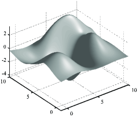
(a) Test Surface $\mathsf{Z}$

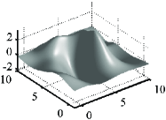
(b) $\mathsf{Z}_{x}$

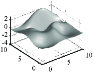
(c) $\mathsf{Z}_{y}$

Figure 3: Ground truth for the Monte-Carlo simulation 3(a) The $150\times 150$ test surface $\mathsf{Z}$ and 3(b), 3(c) its analytic gradient field $\mathsf{Z}_{x}$ and $\mathsf{Z}_{y}$.

The motivation for using such a test function is twofold: the reconstruction can be performed on the analytic derivatives evaluated on a discrete grid; the surface is non-polynomial, which means that only high order derivative approximations will give accurate results. In so doing, the reconstructed surfaces can be compared in terms of relative error with respect to the exact surface, and hence we obtain a quantitative measure of the quality of the surface reconstruction. It should be noted that this is never done in the literature, mainly due to the fact that most published algorithms have some form of systematic error which would skew such results. Therefore, in the literature, it is common to find only subjective reconstruction results, leaving the reader to “eyeball” the quality of the results. The Monte-Carlo experiment, however, is exceptionally illuminating with respect to the insight it gives into the functionality of each algorithm. It is therefore quite peculiar that researchers have yet to perform such experiments. Indeed, with such excessive computation time required for the vectorized solutions, a Monte-Carlo type simulation is all but precluded with previous methods. The Monte-Carlo simulations here, originally proposed in Harker2008c ; harker2011 , thus represent the first ever attempt to benchmark solutions to the reconstruction of a surface from its gradient.
As for the various forms of regularization proposed in this paper, their strengths and weaknesses can be characterized in terms of the type of noise present in the measurement. Hence Monte-Carlo testing has been performed with three types of noise:

1. The gradient field corrupted by i.i.d. Gaussian noise, in which case the GLS algorithm is the “Gold Standard” benchmark solution.

2. The gradient field corrupted by heteroscedastic Gaussian noise, in which case the weighted least squares solution is optimal.

3. The gradient field corrupted by gross-outliers. The outliers are placed randomly throughout the gradient field such that a percentage value of the gradient field is corrupted. Outlier values are set to the maximum value of the respective gradient component to mimic the saturated pixels of an image.

8.2.1 I.I.D. Gaussian Noise

Given the existing methods in the literature, the reconstruction of a surface from a gradient corrupted by i.i.d. Gaussian noise has been, until now, a notoriously difficult problem. Figure 4 shows the gradient of the surface in Figure 3 when corrupted with Gaussian noise with a standard deviation $10\%$ of the gradient amplitude.

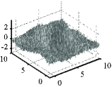
(a) $\mathsf{Z}_{x}$

(b) $\mathsf{Z}_{y}$

Figure 4: Noisy gradient field for the Monte-Carlo simulation, corrupted by i.i.d. Gaussian noise with a standard deviation of $10\%$ of the gradient amplitude.

Figure 5 shows the reconstruction residuals of various existing methods simchony1990 ; kovesi2005 ; agrawal2006 ; horn1986 ; frankot1988 as compared to the new Tikhonov solution. All the existing methods exhibit substantial systematic error in their residuals; in comparison, the new Tikhonov solution has a residual matrix which is purely stochastic – a typical feature of a least squares solution proper. In Figure 6, the histograms of these residuals are plotted. The existing methods exhibit highly irregular distributions due to the systematic errors in their computation. The residuals of the Tikhonov solution presented here are firstly Gaussian, and secondly significantly smaller than those of the state-of-the-art solutions. These are the results one would expect, statistically speaking, from an appropriate global least squares solution. Specifically, in Figure 6 the method of Simchony shows the results of using poor or incorrect derivative formulas; the method of Kovesi (akin to the Frankot-Chellappa method) shows the results of using inappropriate basis functions; and the method of Agrawal et al. shows the general inappropriateness of path integration methods when noise is present in the data. The other methods demonstrate similarly biased results. Similar skewed non-Gaussian residuals are obtained with the FEM type methods such as the method of Balzer and Mörwald balzer2012 . The final “nail-in-the-coffin” of previous methods is demonstrated by means of a Kolomogorov-Smirnov statistical test. Figure 7 shows the normalized distributions of the residuals of various methods. If the methods yield Gaussian residuals, then their density functions should be close to that of a normal distribution. In this case, the residuals of the new method are almost indistinguishable from the normal distribution. In contrast, none of the previous methods come close to a normal distribution. This demonstrates indisputably, that the global least squares surface reconstruction from gradients problem has been, until now, an unsolved problem. In light of the fact that the existing methods have extremely poor noise properties, they have not been included in the subsequent Monte-Carlo tests; namely, their residuals are typically an order of magnitude larger, and hence would obscure any graphical method of comparison.

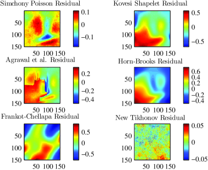
Figure 5: Residuals of various methods: Existing methods exhibit large systematic errors in their residuals. Only the newly proposed methods, such as the Tikhonov regularized solution, exhibit purely stochastic residuals, which one would expect from a least squares solution.

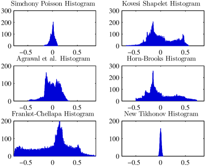
Figure 6: Histograms of the residuals of various methods: only the newly proposed method produces residuals which are themselves Gaussian; note that they are also much smaller in magnitude.

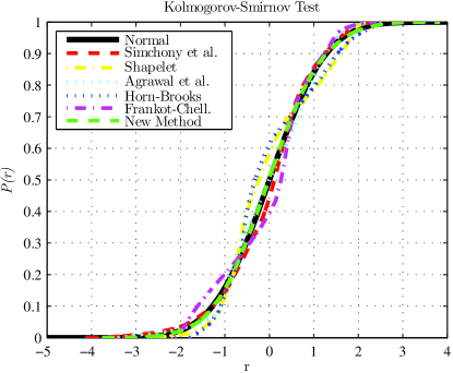
Figure 7: Results from the Kolmogorov-Smirnov test. Clearly, only the new method has Gaussian residuals. This demonstrates definitively that previous methods do not solve the least squares reconstruction problem.

When the gradient field is corrupted by i.i.d. Gaussian noise, the maximum likelihood reconstruction is provided by the least squares solution. That is to say, the “Gold-Standard” in this case is the GLS solution, in that is attains the lowest possible bound of the cost function; it is hence the benchmark solution in the presence of i.i.d. Gaussian noise. The relative value of the cost function attained and the relative reconstruction error are shown for the Monte-Carlo simulation in Figure 8. The lower bound of the cost function is attained by the least squares solution. Notable is the cost function residual of the spectral methods; these have the largest cost function residual, however, they provide the best reconstruction residual. This is due to the fact that the high frequency components have been eliminated, and in this case they correspond to only noise. In contrast, with the least squares solution, this high frequency noise is to some degree integrable. Also of note is the reconstruction with Standard Tikhonov regularization. The reconstruction is not as good because systematic low-frequency errors are suppressed, of which there are none in this case. The degree-2 Tikhonov provides better results as it suppresses the high frequency components. The reconstructed surfaces for the GLS, Spectral-Cosine, and degree-2 Tikhonov methods, all at maximum noise level are shown in Figure 9. The GLS solution exhibits some texture due to the high level of Gaussian noise. The Spectral-Cosine and degree-2 Tikhonov successfully smooth these high frequency components.

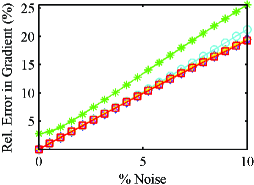
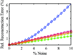
Figure 8: Reconstruction subject to i.i.d. Gaussian noise. (TOP) Relative cost function residual (BOT) Relative Reconstruction Error. Legend: GLS ($\Box$), Spectral-Cosine ($\ast$), Tikhonov Standard Form ($\diamond$), Tikhonov Degree-2 ($\circ$), Weighted Least Squares ($\times$), Dirichlet Boundary Conditions ($+$).

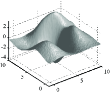
(a) Global Least Squares (GLS)

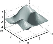
(b) Spectral-Cosine

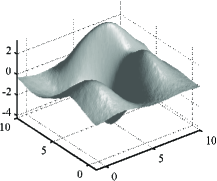
(c) Tikhonov Degree-2

Figure 9: Reconstructions at maximum noise for i.i.d. Gaussian noise 9(a) the GLS solution 9(b) the spectral-cosine reconstruction with half of the basis functions truncated 9(c) Tikhonov reconstruction with degree-2 regularization term.

8.2.2 Heteroscedastic Gaussian Noise

If the noise in the gradient field is anisotropic, then the maximum likelihood solution is given by the weighted least squares solution. For the Monte-Carlo test, the gradient field was corrupted by a radially symmetric noise distribution with increasing noise amplitude towards the image edges; this mimics the error induced in photometric stereo by making the orthographic projection assumption. Results of the Monte-Carlo simulation are shown in Figure 10. Clearly the weighted least squares solution defines the lower bound of the cost function. Again, the standard form Tikhonov regularization provides relatively poor reconstruction since there is no systematic error present. Similarly to the i.i.d. case, the spectral methods have the largest cost function residual, but due to their low-pass functionality, again provide the best reconstruction. In Figure 11, the reconstructions at maximum noise are shown for the weighted least squares, the spectral reconstruction, and Tikhonov degree-1. The Tikhonov degree-1 solution has the effect of suppressing the undulations of the surface, which can have a similar effect as the WLS solution. Clearly in the case of anisotropic noise, a weighted least squares with spectral regularization would provide an optimal solution. This can be accomplished with weighted basis functions oleary2010a .

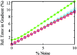
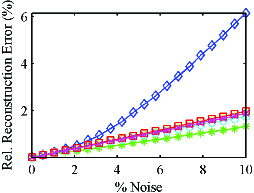
Figure 10: Reconstruction subject to covariant Gaussian noise, in which case weighted least squares is optimal. (TOP) Relative cost function residual (BOT) Relative Reconstruction Error. Legend: GLS ($\Box$), Spectral-Cosine ($\ast$), Tikhonov Standard Form ($\diamond$), Tikhonov Degree-2 ($\circ$), Weighted Least Squares ($\times$), Dirichlet Boundary Conditions ($+$).

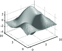
(a) Weighted Least Squares (WLS)

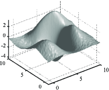
(b) Spectral-Cosine

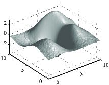
(c) Tikhonov Degree-1

Figure 11: Reconstructions at maximum noise for covariant Gaussian noise 11(a) the WLS solution 11(b) spectral cosine regularization with half the basis functions truncated 11(c) reconstruction with degree-1 Tikhonov regularization.

8.2.3 Gross Outliers

To demonstrate the functionality of the algorithms in the presence of outliers, a Monte-Carlo test was performed based on percentage of outliers. That is, for a given percentage of outliers, random pixels in the gradient were set to the maximum amplitude of the gradient component to simulate saturated image pixels; this simulates what can transpire in real photometric stereo when specular reflection occurs on the object surface. In this case, Tikhonov regularization in standard form (degree-0) algorithm is optimal, since the outliers create a low frequency systematic bias in the solution. Results of the Monte-Carlo simulation are shown in Figure (13), which shows the cost function residual and reconstruction error as a function of percentage of outliers. Clearly the cost function residuals do not follow the linear trend which is typical of a least squares solution subject to Gaussian noise. In the case of the reconstruction error, by far the best reconstruction is provided by the Dirichlet boundary conditions; clearly, if the value of the surface at the boundary is known, the reconstruction can be extremely robust to outliers. The reconstruction with Dirichlet boundary conditions is shown in Figure 12.

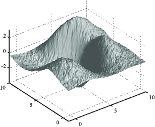
Figure 12: Dirichlet reconstruction with $10\%$ outliers. Given this is an outlandish amount of noise, the Dirichlet reconstruction is shown to be exceptionally robust to outliers.

In this case the low-pass spectral reconstruction is rather poor; however, a band-pass spectral reconstruction can be used to remove low-frequency components largely due to the outliers. The standard form Tikhonov regularization successfully suppresses much of the bias due to the presence of outliers. The reconstruction results at maximum noise (percent outliers) are shown in Figure 14 for low-pass spectral reconstruction, band-pass Spectral-Gram reconstruction, and degree-0 Tikhonov regularization. The large bias of the low-pass spectral reconstruction is evident; the “saturated” outliers induce a large DC component into the gradient, which integrates to a ramp function. However both the band-pass reconstruction (removing all linear polynomial components) and the Tikhonov regularization successfully remove systematic bias from the solution.

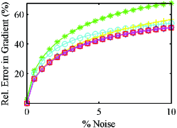
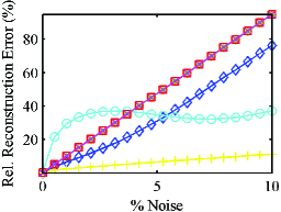
Figure 13: Reconstruction subject gross outliers (saturated gradient pixels). (TOP) Relative cost function residual (BOT) Relative Reconstruction Error. Legend: GLS ($\Box$), Spectral-Cosine ($\ast$), Tikhonov Standard Form ($\diamond$), Tikhonov Degree-2 ($\circ$), Weighted Least Squares ($\times$), Dirichlet Boundary Conditions ($+$).

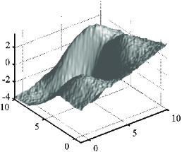
(a) Spectral-Cosine Low-Pass

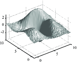
(b) Spectral-Gram Band-Pass

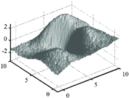
(c) Tikhonov Standard Form

Figure 14: Reconstructions at maximum noise for gross outliers 14(a) Spectral-Cosine with half the basis functions truncated 14(b) Spectral-Gram with half the basis functions truncated as well as the linear components 14(c) Tikhonov Standard form with $\lambda$ determined by the L-Curve.

8.3 Real Photometric Stereo

There are several test data sets in the literature for Photometric Stereo. They are usually photos taken of plaster casts, which are typically very good approximations to Lambertian surfaces. As a consequence, the Photometric Stereo technique yields good approximations to the gradient of the surface. Figure 15 shows the reconstruction results of the so-called “Mozart” data-set. The results presented in agrawal2006 for the same date set demonstrate that until now this data set could have been considered challenging. However, with the global least squares approach presented here this data set can be considered almost trivial due to the Lambertian nature of the test surface.

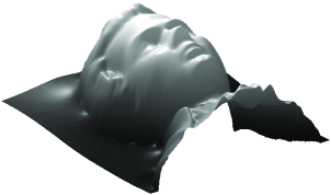
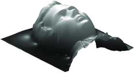
Figure 15: The “Mozart” data set reconstructed with (TOP) the GLS solution and (BELOW) reconstruction with homogeneous Dirichlet boundary conditions on three sides.

What is, however, far more difficult to reconstruct a surface which is non-Lambertian with various different surface textures. Figure 16 shows such a surface whose gradient has been measured via Photometric Stereo. The surface is metallic and has irregular textures such as rust. Thus, the Lambertian assumption will lead to systematic errors in the gradient computation. It is precisely for these such cases that regularization techniques such as Tikhonov Regularization have been developed – for so-called ill-posed problems.

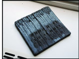
Figure 16: Surface whose gradient was measured via Photometric Stereo.

Figure 17 shows the reconstructions of the surface using the methods proposed in this paper. Figure 17(a) shows the GLS reconstruction, which exhibits a global bending due to inhomogeneities in lighting, among other sources of bias. In Figure 17(b), spectral reconstruction with a band-pass filter is used to remove this bending effect; specifically, all bi-cubic terms are removed from the reconstruction to remove the bending, and the high-frequency components are removed to suppress Gaussian-like noise. Similarly, Tikhonov regularization can be used for the same purpose; in Figure 17(c), Tikhonov regularization in standard form has been used, whilst selecting the regularization parameter, $\lambda_{1}$, using the L-curve method. To show the difficulty in determining the regularization parameter, the result using $\lambda_{2}=3\lambda_{1}$ is shown in Figure 17(d). Clearly this simple change produces a much stronger flattening effect, and the reconstruction appears to be much better in comparison to the original surface. The effects of the weighted least squares solution are more subtle; using an inverted Gaussian-bell like weighting function, the reconstruction errors in the centre of the image are considered more critical. The weighted solution in this case is shown in Figure 17(e), which exhibits systematic differences to the GLS reconstruction, and are more pronounced at the boundaries. Finally, the advantages of applying homogeneous Dirichlet boundary conditions to the reconstruction are shown in Figure 17(f); with the edges of the reconstructed surface essentially simply supported, the low-frequency bending of the surface is almost completely suppressed. Such a reconstruction can be highly effective if the end goal of reconstruction is to automatically read the code stamped on the steel block.

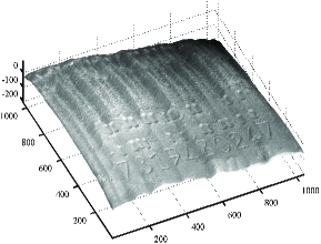
(a) Global Least Squares (GLS)

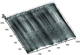
(b) Spectral-Gram Band Pass

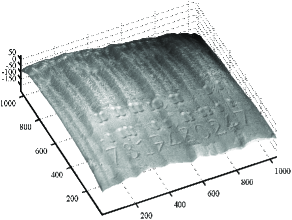
(c) Tikhonov Standard Form $\lambda^{*}$ from L-Curve

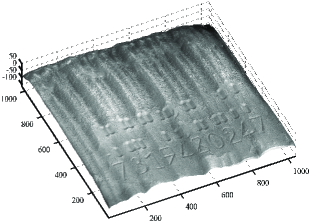
(d) Tikhonov Standard Form $\lambda=3\lambda^{*}$

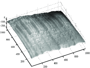
(e) Weighted Least Squares (WLS)

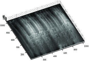
(f) Homogeneous Dirichlet Boundary Conditions

Figure 17: Reconstructions of a real data set obtained via Photometric Stereo 17(a) GLS solution 17(b) Spectral-Gram with all cubic terms removed, as well as the high-frequency half of the basis functions 17(c) Tikhonov Standard Form with $\lambda^{*}$ determined by the L-Curve 17(d) Tikhonov Standard Form but with $\lambda=3\lambda^{*}$ 17(e) Weighted Least Squares 17(f) reconstruction with Homogeneous Dirichlet boundary conditions.

9 Conclusion

This paper presented a framework based on the Sylvester Equation for direct surface reconstruction methods from gradient fields with state-of-the-art forms of regularization. The new algorithms are several orders of magnitudes faster than previous methods due to the efficient solution of Sylvester Equations. A trivial extension of the Framework, would be to combine the various forms of regularization, i.e., Spectral Methods combined with Tikhonov regularization (this has been omitted in the interest of conciseness). Future work will be to further accelerate the solution of the Sylvester Equations; clearly, these too are largely structured and/or sparse. It should also be noted that the Sylvester Equations presented here can be partially solved off-line, and hence may lead to real-time implementations. The methods presented here represent the first viable methods for real-time Photometric Stereo, where regularization is essential, such as in any Industrial Applications.

Appendix A Differentiation of a Frobenius Norm w.r.t. a Matrix

Used frequently throughout this paper is the derivative of the squared Frobenius norm of the general form,

$$f\left(\mathsf{X}\right)=\left\|\mathsf{A}\mathsf{X}\mathsf{B}-\mathsf{C}\right\|_{\textrm{F}}^{2},$$ (133)

with respect to the matrix $\mathsf{X}$. To obtain a formula for the derivative, we firstly define the derivative of the scalar valued function $f=f\left(\mathsf{X}\right)$ with respect to the $m\times n$ matrix $\mathsf{X}$ as the matrix of partial derivatives schoenemann1985 ,

$$\frac{\partial f}{\partial\mathsf{X}}=\left[\frac{\partial f}{\partial x_{ij}}\right].$$ (134)

That is, an $m\times n$ matrix whose $i$-$j$ entry is the partial derivative of $f\left(\mathsf{X}\right)$ with respect to the entries $x_{ij}$ of $\mathsf{X}$. The derivative of the Frobenius norm with respect to the matrix $\mathsf{X}$ is obtained by using the matrix trace definition of the Frobenius norm, i.e.,

$$f\left(\mathsf{X}\right)=\mathop{\mathrm{trace}}\left(\left(\mathsf{A}\mathsf{X}\mathsf{B}-\mathsf{C}\right)\left(\mathsf{A}\mathsf{X}\mathsf{B}-\mathsf{C}\right)^{\textrm{T}}\right)$$ (135)

whereupon expanding yields,

$$f\left(\mathsf{X}\right)=\mathop{\mathrm{trace}}\left(\mathsf{A}\mathsf{X}\mathsf{B}\mathsf{B}^{\textrm{T}}\mathsf{X}^{\textrm{T}}\mathsf{A}^{\textrm{T}}-\mathsf{C}\mathsf{B}^{\textrm{T}}\mathsf{X}^{\textrm{T}}\mathsf{A}^{\textrm{T}}-\mathsf{A}\mathsf{X}\mathsf{B}\mathsf{C}^{\textrm{T}}+\mathsf{C}\mathsf{C}^{\textrm{T}}\right).$$ (136)

Thus, noting that

$$\frac{\partial\mathsf{X}}{\partial x_{ij}}=\boldsymbol{e}_{i}\boldsymbol{e}^{\textrm{T}}_{j},$$ (137)

the derivative of the function with respect to the entry $x_{ij}$ is,

$$\frac{\partial f}{\partial x_{ij}} = \mathop{\mathrm{trace}}\left(\mathsf{A}\boldsymbol{e}_{i}\boldsymbol{e}^{\textrm{T}}_{j}\mathsf{B}\mathsf{B}^{\textrm{T}}\mathsf{X}^{\textrm{T}}\mathsf{A}^{\textrm{T}}+\mathsf{A}\mathsf{X}\mathsf{B}\mathsf{B}^{\textrm{T}}\boldsymbol{e}_{j}\boldsymbol{e}^{\textrm{T}}_{i}\mathsf{A}^{\textrm{T}}\right.$$ (138)

$$- \left.\mathsf{C}\mathsf{B}^{\textrm{T}}\boldsymbol{e}_{j}\boldsymbol{e}^{\textrm{T}}_{i}\mathsf{A}^{\textrm{T}}-\mathsf{A}\boldsymbol{e}_{i}\boldsymbol{e}^{\textrm{T}}_{j}\mathsf{B}\mathsf{C}^{\textrm{T}}\right).$$

Due to the definition of the trace, and the symmetry of its argument, we have,

$$\frac{\partial f}{\partial x_{ij}}=2\mathop{\mathrm{trace}}\left(\mathsf{A}\boldsymbol{e}_{i}\boldsymbol{e}^{\textrm{T}}_{j}\mathsf{B}\mathsf{B}^{\textrm{T}}\mathsf{X}^{\textrm{T}}\mathsf{A}^{\textrm{T}}-\mathsf{A}\boldsymbol{e}_{i}\boldsymbol{e}^{\textrm{T}}_{j}\mathsf{B}\mathsf{C}^{\textrm{T}}\right)$$ (139)

or more simply,

$$\frac{\partial f}{\partial x_{ij}}=2\mathop{\mathrm{trace}}\left(\mathsf{A}\boldsymbol{e}_{i}\boldsymbol{e}^{\textrm{T}}_{j}\mathsf{M}^{\textrm{T}}\right),$$ (140)

where the matrix $\mathsf{M}$ is the placeholder,

$$\mathsf{M}=\mathsf{A}\mathsf{X}\mathsf{B}\mathsf{B}^{\textrm{T}}-\mathsf{C}\mathsf{B}^{\textrm{T}}.$$ (141)

Thus by appropriately indexing the matrices $\mathsf{A}$ and $\mathsf{M}$ we have,

$$\frac{\partial f}{\partial x_{ij}}=2\sum_{k}a_{ki}m_{kj}.$$ (142)

The matrix whose $i$-$j$ entry is this expression is obtained from the rules of matrix multiplication, and hence,

$$\frac{\partial f}{\partial\mathsf{X}}=2\mathsf{A}^{\textrm{T}}\mathsf{M}.$$ (143)

By replacing $\mathsf{M}$ we obtain the desired formula for the derivative of the Frobenius norm,

$$\frac{\partial}{\partial\mathsf{X}}\left\|\mathsf{A}\mathsf{X}\mathsf{B}-\mathsf{C}\right\|_{\textrm{F}}^{2}=2\mathsf{A}^{\textrm{T}}\left(\mathsf{A}\mathsf{X}\mathsf{B}-\mathsf{C}\right)\mathsf{B}^{\textrm{T}}$$ (144)

This identity can be derived using the methods developed in Schönemann schoenemann1985 . All derivatives in this paper can be found using this identity with special cases such as $\mathsf{A}=\mathsf{I}$ or $\mathsf{B}=\mathsf{I}$.

References

- (1) Agrawal, A., Raskar, R., Chellappa, R.: What is the range of surface reconstruction from a gradient field? In: ECCV 2006, pp. 578–591. LNCS, Graz, Austria (2006)
- (2) Balzer, J.: A Gauss-Newton method for the integration of spatial normal fields in shape space. J. Math Imaging Vis 44(1), 65–79 (2011)
- (3) Balzer, J., Mörwald, T.: Isogeometric finite-elements methods and variational reconstruction tasks in vision – A perfect match. In: CVPR 2012, pp. 1624–1631. IEEE, Providence, RI (2012)
- (4) Bartels, R., Stewart, G.: Algorithm 432: Solution of the matrix equation AX + XB = C. Comm. ACM 15, 820–826 (1972)
- (5) Belge, M., Kilmer, M., Miller, E.: Efficient determination of multiple regularization parameters in a generalized L-curve framework. Inverse Problems 18, 1161–1183 (2002)
- (6) Bracewell, R.: The Fourier Transform and its Applications, second edn. McGraw-Hill (1986)
- (7) Burden, R., Faires, J.: Numerical Analysis, eighth edn. Thomson Learning, Inc. (2005)
- (8) Dorr, F.: The direct solution of the discrete Poisson equation on a rectangle. SIAM Rev. 12(2), 248–263 (1970)
- (9) Durou, J.D., Courteille, F.: Integration of a normal field without boundary condition. In: Proc. Workshop on PACV. Rio de Janeiro, Brazil (2007)
- (10) Engl, H., Hanke, M., Neubauer, A.: Regularization of Inverse Problems. Kluwer Academic Publishers, Dordrecht, NL (2000)
- (11) Frankot, R., Chellappa, R.: A method for enforcing integrability in shape from shading algorithms. IEEE PAMI 10(4), 439–451 (1988)
- (12) Golub, G., Meurant, G.: Matrices, Moments and Quadrature with Applications. Princeton University Press, Princeton (2010)
- (13) Golub, G., Nash, S., Van Loan, C.: A Hessenberg-Schur method for the problem AX+XB = C. IEEE Trans. on Automatic Control 24(6), 909–913 (1979)
- (14) Golub, G., Van Loan, C.: Matrix Computations, edn. The Johns Hopkins University Press, Baltimore (1996)
- (15) Gram, J.: Ueber die Entwickelung reeller Functionen in Reihen mittelst der Methode der kleinsten Quadrate. Journal für die reine und angewandte Mathematik 94(1), 41–73 (1883)
- (16) Haar, A.: Zur theorie der orthogonalen funktionensysteme. (erste mitteilung). Mathematische Annalen 69, 331–371 (1910)
- (17) Hansen, P., O’Leary, D.: The use of the L-curve in the regularization of discrete ill-posed problems. SIAM J. Sci. Comput. 14(6), 1487–1503 (1993)
- (18) Harker, M., O’Leary, P.: Least squares surface reconstruction from measured gradient fields. In: CVPR 2008, pp. 1–7. IEEE, Anchorage, AK (2008)
- (19) Harker, M., O’Leary, P.: Least squares surface reconstruction from gradients: Direct algebraic methods with spectral, Tikhonov, and constrained regularization. In: IEEE CVPR, pp. 2529–2536. IEEE, Colorado Springs, CO (2011)
- (20) Higham, N.: Accuracy and Stability of Numerical Algorithms, second edn. SIAM (2002)
- (21) Higham, N.: Computing the nearest correlation matrix – a problem from finance. IMA Journal of Numerical Analysis 22, 329–343 (2002)
- (22) Horn, B., Brooks, M.: The variational approach to shape from shading. Computer Vision, Graphics, and Image Processing 33, 174–208 (1986)
- (23) Horovitz, I., Kiryati, N.: Depth from gradient fields and control points: bias correction in photometric stereo. Image and Vision Computing 22, 681–694 (2004)
- (24) Jaindl, G.: Development of a photometric stereo measurement system. Diploma thesis, University of Leoben (2009)
- (25) Karaçalı B., Snyder, W.: Reconstructing discontinuous surfaces from a given gradient field using partial integrability. Comp. Vis. and Image Underst. 92, 78–111 (2003)
- (26) Karaçalı B., Snyder, W.: Noise reduction in surface reconstruction from a given gradient field. International Journal of Computer Vision 60(1), 25–44 (2004)
- (27) Klette, R., Schlüns, K., Koschan, A.: Computer Vision: Three-Dimensional Data from Images. Springer, Singapore (1998)
- (28) Koskulics, J., Englehardt, S., Long, S., Hu, Y., Stamnes, K.: Method of surface topography retrieval by direct solution of sparse weighted seminormal equations. Optics Express 20(2), 1714–1726 (2012)
- (29) Kovesi, P.: Shapelets correlated with surface normals produce surfaces. In: IEEE ICCV, pp. 994–1001. Beijing (2005)
- (30) Lapidus, L., Pinder, G.: Numerical Solution of Partial Differential Equations in Science and Engineering. John Wiley & Sons, Inc., New York (1999)
- (31) Lee, K., Kuo, C.C.: Surface reconstruction from photometric stereo images. J. Opt. Soc. Am. A 10(5), 855–868 (1993)
- (32) Marquardt, D.: An algorithm for least-squares estimation of nonlinear parameters. J. Soc. Indust. Appl. Math. 11(2), 431–441 (1963)
- (33) Ng, H.S., Wu, T.P., Tang, C.K.: Surface-from-gradients without discrete integrability enforcement: A Gaussian kernel approach. IEEE PAMI 32(11), 2085–2099 (2010)
- (34) O’Leary, P., Harker, M.: An algebraic framework for discrete basis functions in computer vision. In: 2008 ICVGIP, pp. 150–157. IEEE, Bhubaneswar, India (2008)
- (35) O’Leary, P., Harker, M., Neumayr, R.: Savitzky-Golay smoothing for multivariate cyclic measurement data. In: IEEE International Instrumentation and Measurement Technology Conference, pp. 1585–1590. IEEE, Austin, USA (2010)
- (36) Paige, C., Saunders, M.: LSQR: An algorithm for sparse linear equations and sparse least-squares. ACM Transactions on Mathematical Software 8(1), 43–71 (1982)
- (37) Robein, E.: Seismic Imaging: A Review of the Techniques, their Principles, Merits and Limitations. EAGE (2010)
- (38) Robles-Kelly, A., Hancock, E.: A graph-spectral method for surface height recovery. Pat. Rec. 38, 1167–1186 (2005)
- (39) Schönemann, P.: On the formal differentiation of traces and determinants. Multivariate Behavioral Research 20, 113–139 (1985)
- (40) Simchony, T., Chellappa, R., Shao, M.: Direct analytical methods for solving Poisson equations in computer vision. IEEE PAMI 12(5), 435–446 (1990)
- (41) Stewart, G.: Matrix Algorithms, vol. II: Eigensystems. SIAM, Philadelphia (2001)
- (42) Van Loan, C.: The ubiquitous Kronecker product. Journal of Computational and Applied Mathematics 123, 85–100 (2000)
- (43) Woodham, R.: Photometric method for determining surface orientation from multiple images. Optical Engineering 19(1), 139–144 (1980)
- (44) Wu, Z., Li, L.: A line integration based method for depth recovery from surface normals. In: IEEE ICPR, pp. 591–595. IEEE, Rome (1988)