Stability of Z₂ topological order in the presence of vacancy-induced impurity band

Abstract

Although topological insulators (TIs) are known to be robust against non-magnetic perturbations and exhibit edge or surface states as their distinct feature, experimentally it is known that vacancies often occur in these materials and impose strong perturbations. Here we investigate effects of vacancies on the stability of Z₂ topological order using the Kane-Mele (KM) model as a prototype of topological insulator. It is shown that even though a vacancy is not classified as a topological defect in KM model, it generally induces a pair of degenerate midgap states only in the TI phase. We show that these midgap states results from edge states that fit into vacancies and are characterized by the same Z₂ topological order. Furthermore, in the presence of many vacancies, an impurity band that is degenerate with edge states in energy is induced and mixes directly with edge states. However, the Z₂ topological order persists and edge states exist between the impurity band and perturbed bulk bands until a phase transition occurs when Dirac cones near Dirac points are depleted. Our analyses indicate that the same scenario holds for point vacancies or line of vacancies in 3D TIs as well.

I Introduction

Building low dimensional electronic systems has been a focus of intense interest since the discovery of low dimensional materials such as carbon nanotubes and graphene. Recent theoretical and experimental works on topological order of materials Kane ; Hasan ; TI have led to the discovery of a different route to construct low dimensional electronic systems through a new class of materials, called topological insulators (TIs). In these materials, surface states or edge states arise in the boundaries of bulk insulating materials and can host electrons in low dimensions. Depending on the dimension of the materials, a two-dimensional TI hosts one-dimensional gapless edge states while a three-dimensional TI hosts two-dimensional gapless Dirac Fermions. These low dimensional surface states or edges arise from Z₂ topological order of bulk states Kane and are protected by symmetries of bulk states.

Theoretically, the fundamental reason for the emergence of surface states or edge states in TI is due to underlying Z₂ topological structure in the bulk state. Since topological order is protected by associated symmetries symmetry , surface states and edge states in TIs are considered to be robust against bulk disorders that do not break the time-reversal symmetry that is associated with Z₂ topological order. The robustness against disorders is the key to potential technological applications and hence a great effort has been dedicated to understanding the behavior of the topological materials in the presence of disorders Sheng1 ; disorder1 ; disorder2 ; disorder3 ; 3Dstrong ; disorderShen ; Beenakker . Indeed, surface states or edge states are shown to persist in the presence of weak disorders Sheng1 . However, it is also found that in the presence of disorders, anomalous transmutation between TI and insulators with trivial topology may happen 3Dstrong ; disorderShen ; Beenakker . In particular, in computer simulations of a HgTe quantum well, it is discovered that an ordinary insulating state can be transformed into a topological insulator, called topological Anderson insulator disorderShen ; Prodan . The mechanism behind the transformation is shown to be related to the renormalization of Z₂ topological index by disorders near the Dirac points Beenakker and the transformation may also depend on type of disorders Xie . Hence while TI is robust against perturbations, the exact phase boundary for TI may subject to change in the presence of disorders.

Experimentally, it is found that strong perturbations such as lattice defects often occur in topological insulators exptvacancy . From the experience in other similar materials characterized by Dirac Hamiltonian, the presence of lattice defects often induces peculiar properties. In the case of graphene, it was found that vacancies can give rise to magnetic moments and turn graphene into a ferromagnet mou . For topological insulators, it is shown that lattice defects with non-trivial topology also induce bound states lattice . However, in the tetradymite semiconductor Bi₂Se₃ that has been most extensively investigated, the most common observed lattice defects are selenium vacancies, which are not topological defects. These vacancies are believed to give rise to electron doping and increase the conductivity of bulk states dramatically exptvacancy . Furthermore, there are also evidences that vacancies may induce an impurity band that affects current transportation Ando . Since vacancies do not break time-reversal symmetry, their presence is consistent with symmetries that are associated with Z₂ topological order. However, instead of being weak, vacancies are considered as strong perturbations and may change the topological structure of TI. It is therefore interesting and crucial to examine robustness of TI in the presence of vacancies.

In this paper, we will examine the stability of Z₂ topological order in the presence of vacancies using the Kane-Mele model. It is shown that even though vacancies are not classified as topological defects in the Kane-Mele model defect , the original Z₂ topological order insures that midgap bound states are induced only in topologically nontrivial phase. Based on Green’s function analysis of edge states mou1 , we show that these midgap bound states are remanent edge states and form an impurity band in the presence of many vacancies. We shall show that the impurity band coexists with edge states when the Z₂ topological order persists until the spectral weights of Dirac cones near Dirac points are depleted. Finally, we briefly extend our analyses to three dimensions and show that there must be midgap bound states associated with point vacancies or line of vacancies in 3D TIs as well.

II Theoretical formulation and midgap bound states near a vacancy

We start with the Kane-Mele model on a honeycomb lattice. The Hamiltonian is given by Kane

$$H = -t\sum_{<i,j>}c_{i}^{{\dagger}}c_{j}+i\frac{\lambda_{SO}}{3\sqrt{3}}\sum_{<<i,j>>}\nu_{ij}c_{i}^{{\dagger}}\sigma^{z}c_{j}$$ (1)

$$+ i\frac{2\lambda_{R}}{3}\sum_{<i,j>}c_{i}^{\dagger}(\mbox{{\boldmath$\sigma$}}\times{\hat{\mathbf{d}}}_{ij})_{z}c_{j}$$

$$+\lambda_{v}\sum_{i}\mu_{i}c_{i}^{{\dagger}}c_{i}+\sum_{i}V_{i}c_{i}^{{\dagger}}c_{i},$$

where $c_{i}^{{\dagger}}=(c_{i\uparrow}^{{\dagger}},c_{i\downarrow}^{{\dagger}})$ creates an electron at lattice site $i$. The first term accounts for nearest-neighbor hoppings. The second term is a spin-orbit interaction between next nearest neighbors, in which $\nu_{ij}=(2/\sqrt{3})(\hat{d_{1}}\times\hat{d_{2}})\cdot\hat{z}$ with $\hat{d_{1}}$ and $\hat{d_{2}}$ being two nearest-neighbor bonds that connect site $j$ to site $i$, and $\sigma$ are the Pauli matrices. The third term is the Rashba coupling. The fourth term characterizes the sublattice site energies with $\mu_{i}=+1$ $(-1)$ for $i\in A$ ($B$) sites. This term will be considered only in this section. The last term is the random disorder potential that models the impurities, where $V_{i}$ takes a nonvanishing value of $V$ only at impurity sites. In the usual treatment of disorder potential, it often assumes that $V_{i}$ is smooth and is characterized by its correlation function $\langle V_{i}V_{j}\rangle$. Here, however, by taking $V_{i}\rightarrow\infty$, $i$ site is excluded for electrons to visit and hence the limit $V_{i}\rightarrow\infty$ simulates a vacancy at $i$ site. As we shall see, the new ingredient of the lattice vacancy is the possibility of inducing bound states near a vacancy site, which can not be obtained perturbatively by using $\langle V_{i}V_{j}\rangle$. Note that vacancies can be also modeled by cutting all relevant couplings to sites of vacancies and it can be shown that this approach yields the same results in low energy sectors where energy bands occupy. In the following, all energies and lengths will be in units of $t$ and $a$ (lattice constant) respectively.

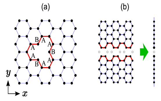
Figure 1: (a) A single vacancy locates at the origin $\vec{r}=(0,0)\equiv\mathbf{0}$, which belongs to $A$ sublattice. (b) A line of point vacancies that are marked by open circles cut an infinite honeycomb lattice into two semi-infinite honeycomb lattices with two edges marked by red lines. After partial Fourier transformation, for each Fourier mode, the system is dimensionally reduced to an effective vacancy in one dimension. Note that curving one of the edges can form a vacancy shown in (a), indicating that mid-gap bound states near a vacancy can be formed by suitable superposition of edge states.

We shall first consider the case of a single vacancy located at the origin $\vec{r}=(0,0)\equiv\mathbf{0}$ that is located at $A$ site. The configuration is shown in Fig. 1(a). According to the classification made Ref. defect , far from a vacancy in 2D, there is no non-trivial winding number associated with the hole introduced by a vacancy and hence a vacancy is not a topological defect. However, this does not imply that there is no midgap bound state associated with a vacancy. In fact, in the continuum limit for HgTe where the Dirac point is at $\Gamma$ point, by approximating a vacancy as a circular hole with radius $R$, it is found that midgap bound states survive with energies being half of the gap magnitude in the limit $R\rightarrow 0$ vacancyShen . In the continuum limit, electrons that occupy the midgap bound states can be viewed as Dirac fermions in a particular curved space Lee . Hence a midgap bound state in a single vacancy results from a superposition of edge states that are curved into the circular surrounding of the vacancy. However, for a vacancy in a honeycomb lattice, the situation is quite different. As shown in Fig. 1(a), a vacancy has a finite size and its surrounding is not in a circular shape. In addition, Dirac points are located at finite wave vectors for honeycomb lattices. It is necessary to examine whether there are midgap bound states associated with vacancies.

To clarify the issue of whether midgap bound states will be induced by a single vacancy, we resort to method of the Green’s function, which has the advantage of not being restricted by finite size effects. In the presence of impurities or vacancies, the Green’s function $G_{\alpha\beta}({\vec{r},\vec{r}^{\prime},E})$ that describes the amplitude for the electron of energy $E$ to propagate from $\vec{r}^{\prime}$ with spin component $\beta$ to the position $\vec{r}$ with spin component $\alpha$ satisfies

$$\left(E-H\right)G({\vec{r},\vec{r}^{\prime},E})=\delta_{\vec{r},\vec{r}^{\prime}},$$ (2)

where we have collectively represented $G_{\alpha\beta}$ by the $2\times 2$ matrix $G$. If we denote the Green’s function in the absence of vacancies by $g({\vec{r},\vec{r}^{\prime},E})$, we find that for a single impurity at $\vec{r}=\mathbf{0}$, $G$ satisfies

$$G({\vec{r},\vec{r}^{\prime},E}) = g({\vec{r},\vec{r}^{\prime},E})+g({\vec{r},\mathbf{0},E})VG({\mathbf{0},\vec{r}^{\prime},E})$$ (3)

$$= g({\vec{r},\vec{r}^{\prime},E})+g({\vec{r},\mathbf{0},E})Tg({\mathbf{0},\vec{r}^{\prime},E}),$$

where $T$ is the T-matrix for a single vacancy at $\vec{r}=\mathbf{0}$ and can be written as

$$T=V+VgV+VgVgV+\cdots=V\left(1-gV\right)^{-1}.$$ (4)

If $H$ supports midgap bound states, $G$ must contain energies of the midgap bound states as poles in $E$. Therefore, the energies of midgap bound states, $E_{0}$, are determined by mou

$$\left.\det\left(1-gV\right)\right|_{E=E_{0}}=0.$$ (5)

In the limit of $V\rightarrow\infty$, the impurity becomes a vacancy. Eq. (5) reduces to equations that determine $E_{0}$ for midgap bound states of vacancies

$$\det g(\mathbf{0},\mathbf{0},E_{0}) = g_{11}\left(\mathbf{0},\mathbf{0},E_{0}\right)g_{22}\left(\mathbf{0},\mathbf{0},E_{0}\right)$$ (6)

$$- g_{12}\left(\mathbf{0},\mathbf{0},E_{0}\right)g_{21}\left(\mathbf{0},\mathbf{0},E_{0}\right)=0,$$

where $1$ and $2$ represent spin up and down respectively. We shall show in below that the existence of a midgap bound state for a single vacancy results from the existence of edge states.

To connect edge states with midgap bound states of a single vacancy, we shall start from a system that is a $Z_{2}$ topological insulator. Hence there are helical edges states for any edges. Furthermore, the energy spectrum of edge states is a Dirac-like spectrum Kane . For a given edge along $\zeta$-direction, since it is translationally invariant along $\zeta$-direction, the system can be dimensionally reduced to one dimension by a partial Fourier transformation along $\zeta$-direction. Let the wave vector along $\zeta$ be $k_{\zeta}$. The existence of edge states thus implies that there are states with energies $E$ being inside the bulk energy gap and being in the form Kane

$$E=\mu_{\zeta}\pm v_{\zeta}k_{\zeta},$$ (7)

where $v_{\zeta}$ is the speed of helical edge states and $\mu_{\zeta}$ is the intersecting energy of two helical modes (energy of the Dirac point). Note that the effective Hamiltonian that gives rise to the helical spectrum of Eq. (7) is a Dirac Hamiltonian and can be written as Kane

$$H_{eff}=\left(\begin{array}[]{cc}\mu_{\zeta}&v_{\zeta}k_{\zeta}\\ v_{\zeta}k_{\zeta}&\mu_{\zeta}\end{array}\right),$$ (8)

where $H_{eff}$ is a $2\times 2$ matrix in the spin space. In the following, we shall show that a midgap bound state for a single vacancy is essentially a weighted superposition of edge states of all possible orientations (denoted by $\zeta$) characterized by Eq. (7).

We now consider creating edges by introducing a line of point vacancies in an infinite honeycomb lattice as illustrated in Fig. 1(b). The vacancy line cuts the infinite honeycomb lattice into two semi-infinite honeycomb lattices with two edges. As we shall show in below, after partial Fourier transformation on coordinates along the vacancy line, for each Fourier mode $k_{\zeta}$, the vacancy line becomes a point. That is, through dimensional reduction, the vacancy line and edge states that are associated with two edges reduce to an effective vacancy with midgap bound states in one dimension. The connection of midgap bound states for a single vacancy to edge states is thus established. From this point of view, we may assume that the vacancy line passes through $\vec{r}=\mathbf{0}$ and its direction is denoted as $\zeta$-direction. Hence the resulting edge for each semi-infinite honeycomb lattice is along $\zeta$-direction. For later usage, we denote the direction perpendicular to $\zeta$ by $\eta$ with the corresponding coordinate being denoted by $x_{\eta}$. In the example shown in Fig. 1(b), one has $\zeta=x$, $\eta=y$, and $k_{\zeta}=k_{x}$. After the partial Fourier transformation along $\zeta$-direction, the Hamiltonian of the whole system (two semi-infinite honeycomb lattices plus a vacancy line) is reduced to one-dimensional subsystems of different $k_{\zeta}$, hence the total Hamiltonian $H$ can be written as

$$H=\sum_{k_{\zeta}}h(k_{\zeta}).$$ (9)

Note that after the partial Fourier transformation, the vacancy line reduces to an effective vacancy for each $k_{\zeta}$, and each $h(k_{\zeta})$ contains a vacancy at the origin of A site, $x_{\eta}=0$. The associated Green’s function is a function of $k_{\zeta}$ and $x_{\eta}$ and can be written as $G_{\alpha\beta}({x_{\eta},x_{\eta}^{\prime},k_{\zeta},E})$. Clearly, following the derivation that leads to Eqs. (3) and (4), since there is a vacancy at $x_{\eta}=0$, we find that for a given $k_{\zeta}$, the T-matrix is given by

$$T(k_{\zeta},E)=V\left(1-g(x_{\eta}=0,x_{\eta}^{\prime}=0,k_{\zeta},E)V\right)^{-1}.$$ (10)

In the limit of $V\rightarrow\infty$, one gets

$$T=-\left[g(x_{\eta}=0,x_{\eta}^{\prime}=0,k_{\zeta},E)\right]^{-1}.$$ (11)

Since edge states are created by the vacancy line, according to Eq. (7), $\mu_{\zeta}\pm v_{\zeta}k_{\zeta}$ must be eigen-energies of $h(k_{\zeta})$ and hence these energies must appear as poles of the T-matrix. In addition, using the fact that edge states are described by the effective Hamiltonian given in Eq. (8) and their energies must be poles of $T$, it implies that

$$T\sim(E-H_{eff})^{-1}.$$ (12)

As a result, by combining Eqs. (11) and (12), we conclude that $g$ will take the following form

$$g(x_{\eta}=0,x^{\prime}_{\eta}=0,k_{\zeta},E)=w(k_{\zeta},E)\left(\begin{array}[]{cc}E-\mu_{\zeta}&v_{\zeta}k_{\zeta}\\ v_{\zeta}k_{\zeta}&E-\mu_{\zeta}\end{array}\right),$$ (13)

where the factor $w(k_{\zeta},E)$ is a proportional constant and accounts for the weight associated with $k_{\zeta}$ mode. Note that $w(k_{\zeta},E)$ is smooth, even in $k_{\zeta}$ and it has no zeros in $E$.

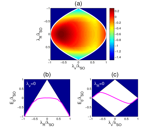
Figure 2: (Color online) Energies ($E_{0}$) of mid-gap bound states induced by a single vacancy. (a) Color map of $E_{0}/\lambda_{SO}$. Mid-gap bound states only appear inside the TI phase. The region outside the TI phase (enclosed by the white line) is marked as blue to indicate that there is no mid-gap bound state. (b) and (c) show energies of mid-gap bound states along axes at $\lambda_{v}=0$ and $\lambda_{R}=0$, respectively. Regions marked by blue are for band states. It is seen that energies of mid-gap bound states approach band edges when boundaries of the TI phase are approached.

Using Eq. (13), the origin of the vacancy state is made clear. We first note that the bulk Green’s function in Eq. (6) satisfies

$$g(\mathbf{0},\mathbf{0},E)=\sum_{k_{\zeta}}g(x_{\eta}=0,x_{\eta}^{\prime}=0,k_{\zeta},E).$$ (14)

Combining Eqs. (13) and (14), we find

$$g(\mathbf{0},\mathbf{0},E)=\left(\begin{array}[]{cc}w_{t}E-\mu_{t}&0\\ 0&w_{t}E-\mu_{t}\end{array}\right),$$ (15)

where $w_{t}=\sum_{k_{\zeta}}w$, $\mu_{t}=\sum_{k_{\zeta}}w\mu_{\zeta}$ and we have made use the fact that the summation $\sum wk_{\zeta}$ vanishes due to that $w(k_{\zeta},E)$ is an even function of $k_{\zeta}$. Eq. (15) then yields two midgap bound states with a degenerate energy at

$$E_{0}=\bar{\mu}_{\zeta}\equiv\frac{\sum_{k_{\zeta}}w\mu_{\zeta}}{\sum_{k_{\zeta}}w}.$$ (16)

Here $\bar{\mu}_{\zeta}$ is the weighted average of the intersecting energy for two helical modes and hence it must lie inside the gap

$$|\mu_{\zeta}|<\Delta_{\zeta},$$ (17)

where $\Delta_{\zeta}$ is the gap along $\zeta$-direction. In the TI phase, since there are edge states inside the energy gap for all orientations of edges, $E$ must satisfy Eq. (17) for all possible $\zeta$, including the minimum of $\Delta_{\zeta}$, which is the energy of the system. Hence one concludes that in consistent with the Kramers degeneracy theorem, there must be a pair of degenerate vacancy states inside the energy gap in the TI phase.

To verify the above conclusion, we evaluate energies of midgap bound states induced by a single vacancy through solving Eq. (6) numerically. Figure 2 shows energies of midgap bound states induced by a single vacancy. It is seen that generally the midgap bound energy $E_{0}$ is not fixed to zero and depends on values of parameters $\lambda_{R}$ and $\lambda_{SO}$. As one approaches boundaries of the TI phase, $E_{0}$ moves towards edges of band gap. In the trivial insulator phase, the midgap bound state merges into the bulk band and become a resonant state. Hence we conclude that only the TI phase supports midgap bound states.

III Impurity band and its effects on topological characterization

In this section, we investigate effects of vacancies on Z₂ topological order. For this purpose, we shall first investigate the distribution of states induced by vacancies. In Fig. 3(a), we show typical changes of density of states for the system in the presence of a single impurity when $V$ increases from $0$ to a very large magnitude. It is seen that two midgap bound states degenerate in energy emerge from the band edge and settles at a fixed energy inside the energy gap when $V$ approaches $\infty$. Furthermore, it is shown that whenever a midgap bound state is induced, a high energy state at $E\sim V$ is also induced at the same time. The high energy state is localized precisely at the impurity site and is pushed to infinity when $V$ goes to $\infty$. Therefore, each vacancy induces two midgap states degenerated at one midgap energy. When there are $M$ vacancies at random positions, $M$ midgap energies are induced. Figure 3(b) shows that as the number of vacancies increases, these midgap bound states start to form an impurity band inside the gap. The appearance of an impurity band is in agreement with the observation made in Ref. Ando . These midgap states are localized states. Note that since the system is composed by spin-1/2 electrons with time-reversal symmetry and without spin-rotation symmetry, disordered topological insulators belong to symplectic symmetry class Furusaki . The level statistics of midgap energies is thus characterized by the so-called Gaussian sympletic ensemble Mehta . In particular, for a Gaussian sympletic ensemble, the level-spacing distribution follows Wigner-Dyson type distribution Mehta . Hence for midgap energies in the impurity band, the distribution of level spacings also follows the Wigner-Dyson distribution.

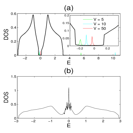
Figure 3: (Color online) Typical density of states for a single impurity (a) and for many vacancies (b). Here energies are in unit of $t$, $\lambda_{R}=0.075$, and $\lambda_{SO}=0.18\sqrt{3}$. The vacancy density in (b) is $1/9$. It is seen that an impurity band emerges for finite density of vacancies, in agreement with the observation of Ref. Ando .

From Fig. 3(a), we have the following counting for level distribution. In a honeycomb lattice with the number of unit cells being $N$, there are $2N$ lattice points and the total number of states is $4N$. If there are $M$ vacancies, the distribution of energies is as follows

$$\mathrm{{Level~{}~{}counting}\left\{\begin{array}[]{l}{valence~{}~{}band:~{}~{}}2N-M\\ {impurity~{}~{}band:~{}~{}}M\\ {conduction~{}~{}band:~{}~{}}2N-M\\ {high~{}~{}energy~{}~{}states:~{}~{}}M.\end{array}\right.}$$ (18)

By using the above level distribution, one can characterize the Z₂ topological index for each band. For this purpose, we first note that the defining property of the non-trivial Z₂ topological index is the Quantum spin Hall effect (QSHE). Therefore, the Z₂ topological index can be evaluated by computing quantum spin Hall conductance (QSHC). Computing the Z₂ index by evaluating QSHC is particularly useful when there is no translational invariance in the presence of vacancies and one can not define electronic Bloch states. To calculate QSHC, generally one imposes spin-dependent twisted boundary conditions Sheng107 as

$$c_{j+N_{x}\hat{x}}^{\alpha}=e^{i\theta_{x}^{\alpha}}c_{j}^{\alpha},$$

$$c_{j+N_{y}\hat{y}}^{\beta}=e^{i\theta_{y}^{\beta}}c_{j}^{\beta}.$$ (19)

Here $\alpha,\beta=\pm 1$ are the spin indices that represent the spin state of $\uparrow$ and $\downarrow$ respectively. $j$ specifies the site, $N_{x}$ and $N_{y}$ are numbers of sites along $x$ and $y$ directions respectively [refer to Fig. 1(a)], and $\theta_{x}^{\alpha}$ ($\theta_{y}^{\beta}$) are phases acquired whenever an electron with spin component $\alpha$ ($\beta$) goes across the boundary along $x$ ($y$) directions respectively. Both $\theta_{x}^{\alpha}$ and $\theta_{y}^{\beta}$ are in the range $[0,2\pi]$. Following Ref. Sheng107 , when the degeneracy between spin state $+1$ and $-1$ is lifted, the Hall conductances are generally represented as $\sigma_{xy}^{\alpha\beta}$ which characterizes the Hall voltage in the $x$ direction due to electrons of spins component $\alpha$ when the spin-polarized current with spin component $\beta$ flows in the $y$ direction. The topological Chern number that is associated with $\sigma_{xy}^{\alpha\beta}$ is thus defined as Sheng107

$$C_{\alpha\beta}=\frac{i}{4\pi}\int\int d\theta_{x}^{\alpha}d\theta_{y}^{\beta}\left[\langle\frac{\partial\psi}{\partial\theta_{x}^{\alpha}}|\frac{\partial\psi}{\partial\theta_{y}^{\beta}}\rangle-\langle\frac{\partial\psi}{\partial\theta_{y}^{\beta}}|\frac{\partial\psi}{\partial\theta_{x}^{\alpha}}\rangle\right],$$ (20)

where $\psi$ is the many-particle ground state wavefunction of the system. $C_{\alpha\beta}$ can be collectively represented as a $2\times 2$ matrix, representing the non-Abelian nature of the Hall conductance. For the quantum Hall effect (QHE), it is entirely due to charges. The Hall conductance of QHE is given by $\sigma_{H}=\sum_{\alpha,\beta}\sigma_{xy}^{\alpha\beta}$. Hence it is clear that $\sum_{\alpha,\beta}C_{\alpha\beta}$ is the corresponding Chern number associated with QHE. On the other hand, the QSHE is defined as the difference of Hall conductances between spin $\uparrow$ and $\downarrow$. The QSHC $\sigma_{sH}$ is then given by

$$\sigma_{sH}=\sum_{\beta}\sigma_{xy}^{+\beta}-\sum_{\beta}\sigma_{xy}^{-\beta}=\sum_{\alpha\beta}\alpha\sigma_{xy}^{\alpha\beta}.$$ (21)

As a result, the corresponding spin Chern number that is associated with QSHE is given by

$$C_{s}=\sum_{\alpha\beta}\alpha C_{\alpha\beta}.$$ (22)

From Eqs. (20) and (22), it is seen that the minus sign associated with down spin can be absorbed into the twisted phase $\theta_{x}^{\downarrow}$ so that one can set $\theta_{x}^{\downarrow}=-\theta_{x}^{\uparrow}$. Therefore, to focus on the spin Chern number, one sets $\theta_{y}^{\uparrow}=\theta_{y}^{\downarrow}=\theta_{y}$ and $\theta_{x}^{\uparrow}=-\theta_{x}^{\downarrow}=\theta_{x}$ and imposes the spin-dependent twisted boundary conditions Sheng107 ; Hatsugai2 as follows

$$c_{j+N_{x}\hat{x}}=e^{i\theta_{x}\sigma_{z}}c_{j},$$

$$c_{j+N_{y}\hat{y}}=e^{i\theta_{y}}c_{j},$$ (23)

where $\sigma_{z}$ is the $z$ component of the Pauli matrices and both $\theta_{x}$ and $\theta_{y}$ are in the range $[0,2\pi]$. The gauge potential $\Phi$ imposed by twisted boundary conditions is

$$\Phi(i_{x},i_{y})=\sigma_{z}\frac{\theta_{x}i_{x}}{N_{x}}+\frac{\theta_{y}i_{y}}{N_{y}}.$$ (24)

Due to the presence of $\sigma_{z}$, $\Phi$ does not commute with $H$, which reflects the non-Abelian nature of the problem. Note that the spin Chern number computed by the spin-dependent twisted boundary conditions has been rigorously shown to be equivalent to the Z₂ topological index Hatsugai2 ; Vanderbilt .

Following Refs. Hatsugai1 and Hatsugai2 , using the energy eigenkets of $H$ with spin-dependent twisted boundary conditions, one can compute the spin Chern number which yields the same classification as that of Z₂ topological order. For this purpose, we discretize the space $[0,2\pi]\times[0,2\pi]$ into $M\times M$ mesh points so that a general twisted boundary condition is represented by $\theta\equiv(\theta_{p},\theta_{q})$ with $\theta_{p}=2\pi p/M$, $\theta_{q}=2\pi q/M$ and $p,q=0,1,2,3,\cdots,M-1$. For each $\theta$, since hopping across boundaries depends on $\theta$, the Hamiltonian depends on $\theta$, $H(\theta)$, with eigenstates being $|n(\theta)\rangle$. For each bond that connects $\theta$ and $\theta+\delta\theta_{i}\hat{\imath}$ with $\delta\theta_{i}=2\pi/M$ and $i=x$ or $y$, a non-Abelian link variable $U_{i}(\theta)$ is defined as the overlap matrix

$$U_{i}(\theta)_{mn}=\langle m(\theta)|n(\theta+\delta\theta_{i}\hat{\imath})\rangle,$$ (25)

where $n$ and $m$ are indices of energy bands that are included for computing the spin Chern number. From the link variable $U_{i}(\theta)$, a U(1) link $u_{i}(\theta)$ can be formed

$$u_{i}(\theta)=\det U_{i}(\theta)/|\det U_{i}(\theta)|.$$ (26)

One can then find the lattice field strength $F_{xy}$ for each plaquette in the $(\theta_{x},\theta_{y})$ lattice by computing

$$F_{xy}(\theta) = \ln\left[u_{x}(\theta)u_{y}(\theta+\delta\theta_{x}\hat{x})\right.$$

$$\left.u_{x}^{-1}(\theta+\delta\theta_{x}\hat{x}+\delta\theta_{y}\hat{y})u_{y}^{-1}(\theta+\delta\theta_{y}\hat{y})\right],$$

where the principle branch of logarithm is taken. The spin Chern number is the summation of $F_{xy}$ over all plaquettes given by

$$C_{s}=\frac{1}{2\pi i}\sum_{\theta}F_{xy}(\theta).$$ (28)

The spin Chern number thus obtained is always an integer. Furthermore, it has the advantage of being accurate even when the computation is done with small sizes of honeycomb lattices Hatsugai1 ; Hatsugai2 .

To characterize TI with vacancies at random positions, we compute $C_{s}$ for valence band, impurity band and conduction band. For a given density of vacancies, it is found that depending on the configuration of positions for vacancies, the spin Chern number of each band can be either $2$ or $0$. As a result, one has to perform average of $C_{s}$ over configurations of vacancies. However, we find that as long as there is no overlap between these bands, $C_{s}$ of the impurity band always vanishes. Hence $C_{s}$ of the conduction band is always opposite to that of the valence band.

To confirm the validity of computed $C_{s}$ based on Eq. (28), for a given vacancy configuration, we examine the bulk-edge correspondence by computing the energy spectrum for honeycomb ribbons with the armchair edges. To this end, it is convenient to compute the spectral function $A(\vec{k},\omega)$ defined by

$$A(\vec{k},\omega)=-\frac{1}{N\pi}\rm{Im}\left\{\sum_{j=1}^{4}\sum_{n,m=1}^{4N}\frac{|\langle n|\psi(\vec{k},j,m)\rangle|^{2}}{(\omega-E_{n})+i\Gamma}\right\},$$ (29)

where $\Gamma$ is an energy scale characterizing energy resolution, $|n\rangle$ is the n-th energy eigenstate of the impure system with eigen-energy $E_{n}$, and $|\psi(\vec{k},j,m)\rangle$ is the energy eigenstate in the absence of vacancy with $\vec{k}$ being the wave vector after Fourier transformation. Figure 4 shows the spectral function $A$ of a honeycomb ribbon with armchair edges in the presence of vacancies for different vacancy densities. Here the listed spin Chern numbers are computed by using Eq.(28) based on twisted boundary conditions. The armchair edges are along the $x$ direction so we have the conserved wave vector $k_{x}$. It is seen that for small vacancy densities when $C_{s}$ does not vanish for both valence and conduction bands, edges states exist and coexist with the impurity band at the center. Furthermore, in consistent with the bulk-edge correspondence, edge states reside between the impurity band and the valence band or the conduction band. As the density of vacancies increases, the strength of the impurity band increases and eventually $C_{s}$ for all energy bands vanish. In this case, as shown in Fig. 4(c), edge states diminish as well.

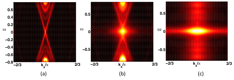
Figure 4: (Color online) Coexistence of edge states and the impurity band exhibited in the spectral function $A(k_{x},\omega)$ of a honeycomb ribbon with armchair edges for different vacancy densities: (a) 0% ($C_{s}=2$ for the valence band, $C_{s}=-2$ for the conduction band) (b) 3% ($C_{s}=2$ for valence band, $C_{s}=0$ for the impurity band, $C_{s}=-2$ for the conduction band) (c) 30% ($C_{s}=0$ for all energy bands). Here $k_{x}$ is the wave vector along armchair edges, $\Gamma=0.01$, $\lambda_{R}=0.075$, $\lambda_{SO}=0.18\sqrt{3}$, and the size of the honeycomb ribbon is $100\times 8$. Here the listed spin Chern numbers are computed by using Eq.(28) based on twisted boundary conditions.

As indicated in the above, to explore the nature of transition, it is necessary to compute the averaged spin Chern number. In Fig. 5, we show the averaged spin Chern number for the valence band of TIs in the presence vacancies which positions are only at A sites or distribute equally at A sites and B sites. The validity of computations based on Eq.(28) is also checked by direct computation of the corresponding systems with open boundaries. It is seen that a phase transition from TI to a trivial insulator occurs as density of vacancies increases. However, depending on positions of vacancies, the transition can be either first order when vacancies are randomly chosen at A sites or continuous when vacancies are randomly chosen equally at A sites or B sites. As we shall explore in the following, the mechanism that causes different transition behaviors lies in the speed of the Dirac cones being depleted. Since the formation of Dirac cones involves with both A sites and B sites, removing points in A sites and B sites simultaneously will start to deplete the Dirac cone and the depletion is proportional to the number of points being removed. As a result, the transition is continuous when vacancies are distributed equally at A sites and B sites. On the other hand, removing points solely at A sites does not deplete the Dirac cone immediately at first until when too many A points are removed, the bi-partite nature is destroyed. At that point, further increase of vacancies induces a discontinuous transition to a trivial insulator with $C_{s}=0$.

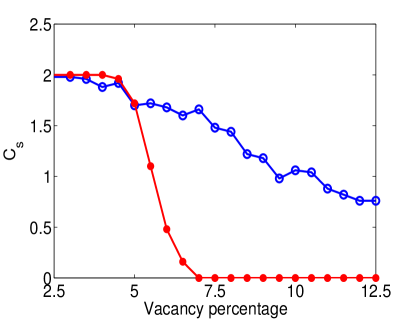
Figure 5: (Color online) Phase transition of TI to a trivial insulator due to the presence of vacancies at random positions. Here the averaged spin Chern number ($C_{s}$) is computed for the valence band with vacancies being located only at A sites (solid circle) or equally distributed at A sites and B sites (open circle). Parameters in the plot are $M=10$, $\lambda_{R}=0.075$, $\lambda_{SO}=0.18\sqrt{3}$, and the average is taken over $100$ vacancy configurations.

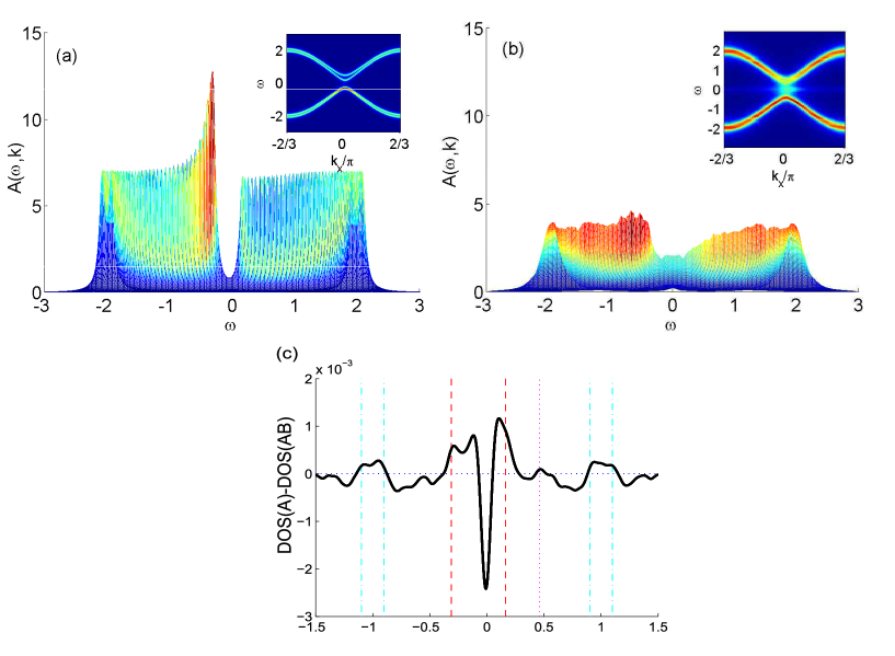
Figure 6: (Color online) Depletion of Dirac cones exhibited in $A(k,\omega)$ and the density of states. Here (a) and (b) show the side view of $A(k,\omega)$ along $\omega$ axis for a honeycomb lattice of size 100 $\times$ 8 with different number of vacancies: (a) 0% (b) 6.26%. A sharp peak at Dirac point is clearly revealed in (a) but is depleted quickly when vacancies are introduced, as shown in (b). (c) Difference of densities of states for 20 vacancies in a 50$\times$50 honeycomb lattice with vacancies being solely distributed at A sites, DOS(A), and vacancies being distributed equally at A sites and B sites, DOS(AB). Here $\lambda_{R}=0.075$, and $\lambda_{SO}=0.18\sqrt{3}$. Dashed and dotted lines indicate energy of gaps at Dirac points, while dot-dashed lines indicate energies at M points. It is seen that the Dirac cones are less depleted when vacancies are solely distributed at A sites.

To explore the mechanism of how Z₂ topological order is destroyed by vacancies, we first note that near the phase boundary when the energy gap vanishes, the dominant contribution of the spin Chern number is from $k$ points near the Dirac points due to the singularity induced by band touching of conduction and valence bands. It is known that the Dirac cones continue to dominate the contribution of Z₂ topological order even when the system is away from the phase boundary Ezawa . Therefore, it is essential to examine how Dirac cones evolve with the introduction of vacancies. For this purpose, we examine the spectral function $A(\vec{k},\omega)$ near Dirac cones using the periodic boundary conditions so that the spectral weight only reflects effects due to vacancies not due to edge states. In Fig. 6(a), we show side view of $A(\vec{k},\omega)$ of a honeycomb lattice in the TI phase with a size of 100$\times$8. A clear peak located right at the Dirac point is exhibited. The peak that reflects the spectral weight near Dirac cones is depleted quickly once vacancies are introduced, as shown in Fig. 6(b). Here the number of vacancies is 90, i.e., density of vacancies is 6.25%. Clearly, it shows that the diminishing of $C_{s}$ correlates with the depletion of Dirac cones. To further differentiate effects due to distribution of vacancies on different sub-lattices, we compute the density of states for 20 vacancies in a 50$\times$50 honeycomb lattice with vacancies being solely distributed at A sites, denoted by DOS(A), and vacancies be distributed equally at A sites and B sites, denoted as DOS(AB). The difference of densities of states is shown in Fig. 6(c). Clearly, the difference, DOS(A)-DOS(AB), is pronounced at several energies. Here dashed and dotted lines indicate energies of gaps at Dirac points (K point), while dot-dashed lines indicate energies at M points. It is seen that removing points solely at A sites tends to keep a higher spectral weight at symmetry points (K and M points) in $k$ space. As a result, the Dirac cones are less depleted when vacancies are distributed solely at A sites. The analyses shown here show that direct depletion of the Dirac cones is the main mechanism for transition from the TIs to trivial insulators for low concentrations of vacancies. For higher concentration of vacancies, as shown in Fig. 4, the impurity band starts to overlap with energy bands and destructs of Z2 topological order eventually.

IV Discussion and conclusion

In summary, we have shown that vacancies in the TI phase of the Kane-Mele model always induce midgap bound states. These midgap bound states result from curving edge states into the surroundings of vacancies. The same reasoning can be generalized to investigate point vacancies or line vacancies in 3D TIs. In this case, the T-matrix still obeys Eq. (4). By introducing a plane of vacancies passing through $\vec{r}=\mathbf{0}$ that cuts infinite 3D lattice into two semi-infinite 3D lattices and following similar considerations that lead to Eq. (14), one arrives at

$$g(\mathbf{0},\mathbf{0},E)=\sum_{k_{\alpha},k_{\beta}}g(x_{\gamma}=0,x_{\gamma}^{\prime}=0,k_{\alpha},k_{\beta},E),$$ (30)

where $k_{\alpha}$ and $k_{\beta}$ are wave vectors in two orthogonal directions of the plane with vacancies and $x_{\gamma}$ is the coordinate of the axis in perpendicular to the plane. For 3D TIs, since there are midgap surface states characterized by spectrum $\pm v_{\parallel}k_{\parallel}+\mu_{\parallel}$ with $k_{\parallel}=\sqrt{k_{\alpha}^{2}+k_{\beta}^{2}}$, the same reasoning leads to the conclusion that in the low energy sector, $g$ must take the following form

$$g(0_{\gamma},0_{\gamma},k_{\alpha},k_{\beta},E)=$$

$$w(k_{\alpha},k_{\beta},E)\left[\begin{array}[]{cc}E-\mu_{\parallel}&v_{\parallel}(k_{\alpha}-ik_{\beta})\\ v_{\parallel}(k_{\alpha}+ik_{\beta})&E-\mu_{\parallel}\end{array}\right],$$ (33)

where $v_{\parallel}$ is the speed of electrons in surface states, $\mu_{\parallel}$ is the energy of the Dirac point, and $w(k_{\alpha},k_{\beta},E)$ is the weight associated with $k_{\parallel}$ and is a smooth function of $E$. Hence we arrive at a conclusion similar to Eq. (17) with $\Delta_{\zeta}$ being replaced by the gap $\Delta_{\parallel}$ of $\vec{k}$ that lies in directions perpendicular to $\gamma$. As a result, one also concludes that there must be a pair of degenerated states inside the energy gap for a single vacancy in 3D topological insulators. This conclusion is in agreement with direct numerical simulations investigated in Ref. Balatsky . Similarly, for a singe line of vacancies along $\delta$ direction, performing a partial Fourier transform on the Hamiltonian along $\delta$ reduces the problem to a 2D problem with a point vacancy. Hence there must be a pair of degenerated states inside the energy gap for every $k_{\delta}$ mode along each line of vacancies in 3D TIs.

In addition to showing that midgap bound states must arise in the presence of a single vacancy, we also show that an impurity band emerges when the number of vacancies increases. The impurity band mixes directly with edge states. However, the impurity band always has trivial topological structure and the Z ₂ topological order persists in both the conduction band and the valence band. Hence edge states exist between the impurity band and perturbed conduction or valence band. The mechanism behind the transition from TI to a trivial insulator due to vacancies is shown to be resulted from the depletion of Dirac cones. Furthermore, due to different speeds of depleting Dirac cones, the transition can be either first order when vacancies are randomly chosen at A sites or continuous when vacancies are randomly chosen equally at A sites or B sites.

While so far in this work we only consider effects of vacancies, our results are not restricted to the limit $V\rightarrow\infty$. For finite and large $V$, Eq. (6) is modified with a correction of $O(1/V)$. Hence midgap bound states induced by vacancies are shifted by the order of $O(1/V)$, in agreement with results shown in Fig. 3. The phase boundary for midgap bound states shown in Fig. 2 then remains the same. As a result, the impurity band is also shifted by a similar amount. The majority of our results remains valid and provides useful characterization of electronic states induced by point defects in TIs.

- (1) C. L. Kane and E. J. Mele, Phys. Rev. Lett. 95, 146802 (2005); L. Fu, C. L. Kane, and E. J. Mele, ibid. 98, 106803 (2007).
- (2) M. Z. Hasan and C. L. Kane, Rev. Mod. Phys. 82, 3045 (2010).
- (3) See X. L. Qi and S.-C. Zhang, Rev. Mod. Phys. 83, 1057 (2011) and reference therein.
- (4) A. P. Schnyder, S. Ryu, A. Furusaki, and A. W. W. Ludwig, Phys. Rev. B 78, 195125 (2008).
- (5) D. N. Sheng, Z. Y. Weng, L. Sheng, and F. D. M. Haldane, Phys. Rev. Lett. 97, 036808 (2006).
- (6) M. Onoda, Y. Avishai, and N. Nagaosa, Phys. Rev. Lett. 98, 076802 (2007).
- (7) A. M. Essin and J. E. Moore, Phys. Rev. B 76, 165307 (2007).
- (8) H. Obuse, A. Furusaki, S. Ryu, and C. Mudry, Phys. Rev. B 76, 075301 (2007); H. Obuse, A. Furusaki, S. Ryu, and C. Mudry, ibid. 78, 115301 (2008).
- (9) G. Schubert, H. Fehske, L. Fritz, and M. Vojta, Phys. Rev. B 85, R201105, (2012).
- (10) J. Li, R. L. Chu, J. K. Jain, and S. Q. Shen, Phys. Rev. Lett. 102, 136806 (2009).
- (11) E. Prodan, Phys. Rev. B 83, 195119 (2011).
- (12) C. W. Groth, M. Wimmer, A. R. Akhmerov, J. Tworzydlo, and C. W. J. Beenakker, Phys. Rev. Lett. 103, 196805, (2009).
- (13) J. Song, H. Liu, H. Jiang, Q. F. Sun, and X. C. Xie, Phys. Rev. B 85, 19512, (2012).
- (14) Y. S. Hor et al., Phys. Rev. B 79, 195208 (2009); P. Cheng et al., Phys. Rev. Lett. 105, 076801 (2010).
- (15) B. L. Huang and C. Y. Mou, Europhys. Lett. 88, 68005, (2009); B. L. Huang, M. C. Chang, and C. Y. Mou, Phys. Rev. B 82, 155462 (2010).
- (16) A. Rüegg and C. Lin, Phys. Rev. Lett. 110, 046401 (2013); Y. Ran, arXive: 1006.5454; Y. Ran, Y. Zhang, and A. Vishwanath, Nature Phys. 5, 298 (2009).
- (17) Z. Ren, A. A. Taskin, S. Sasaki, K. Segawa, and Y. Ando, Phys. Rev. B 82, 241306(R) (2010).
- (18) J. C. Y. Teo, L. Fu, and C. L. Kane, Phys. Rev. B 78, 045426 (2008).
- (19) S. T. Wu and C. Y. Mou, Phys. Rev. B 66 012512 (2002); C. Y. Mou, R. Wortis, A. T. Dorsey, and D. A. Huse, Phys. Rev. B 51, 6575 (1995); S. T. Wu and C. Y. Mou, Phys. Rev. B 67, 024503 (2003).
- (20) W. Y. Shan, J. Lu, H. Z. Lu, and S. Q. Shen, Phys. Rev. B 84, 035307 (2011).
- (21) D. H. Lee, Phys. Rev. Lett. 103, 196804 (2009).
- (22) S. Ryu, C. Mudry, H. Obuse, and A. Furusaki, Phys. Rev. Lett. 99, 116601, (2007).
- (23) M. L. Mehta, Random Matrices, (Elsevier/Academic Press, San Diego, 2004).
- (24) D. N. Sheng, Z.Y. Weng, L. Sheng, and F.D.M. Haldane, Phys. Rev. Lett. 97, 036808 (2006); Y. Yang, Z. Xu, L. Sheng, B. Wang, D.Y. Xing, and D. N. Sheng, ibid. 107, 066602 (2011).
- (25) T. Fukui, Y. Hatsugai, and H. Suzuki, J. Phys. Soc. Jpn. 74, 1674 (2005).
- (26) T. Fukui and Y. Hatsugai, Phys. Rev. B 75, 121403(R) (2007).
- (27) A. A. Soluyanov and D. Vanderbilt, Phys. Rev. B 85, 115415 (2012).
- (28) M. Ezawa, Phys. Rev. Lett. 109, 055502 (2012).
- (29) A. M. Black-Schaffer and A. V. Balatsky, Phys. Rev. B 85, 121103(R) (2012); 86, 115433 (2012).