Majorana modes in smooth normal-superconductor nanowire junctions

Abstract

A numerical method to obtain the spectrum of smooth normal-superconductor junctions in nanowires, able to host Majorana zero modes, is presented. Softness in the potential and superconductor interfaces yields opposite effects on the protection of Majorana modes. While a soft potential is a hindrance for protection, a soft superconductor gap transition greatly favors it. Our method also points out the possibility of extended Majorana states when propagating modes are active far from the junction, although this requires equal incident fluxes in all open channels.

I Introduction

In 1936 Ettore Majorana theorized the existence of elementary particles, now called Majorana Fermions, that coincide with their own antiparticles.Majorana (1937) The implementation of quasiparticle excitations having a similar property, called Majorana states, is currently attracting much interest in condensed matter systems in general,Kitaev (2001); Wilceck (2009); Alicea (2012); Qi and Zhang (2011); Leijnse and Flensberg (2012); Beenakker (2013); Stanescu and Tewari (2013a); Fu and Kane (2008); Akhmerov et al. (2009); Tanaka et al. (2009); Law et al. (2009) and in nanowires in particular.Lutchyn et al. (2010); Oreg et al. (2010); Stanescu et al. (2011); Flensberg (2010); Potter and Lee (2010, 2011); Gangadharaiah et al. (2011); Egger et al. (2010); Zazunov et al. (2011); Klinovaja et al. (2012); Klinovaja and Loss (2012); Lim et al. (2012a, b, 2013) Interest has been further fueled by recent experimental evidences of these Majorana states in quantum wires.Mourik et al. (2012); Deng et al. (2012); Rokhinson et al. (2012); Das et al. (2012); Finck et al. (2013) They are also known as Majorana zero modes (MZM) and, in essence, they are topological zero-energy states living close to the system edges or interfaces. The existence of an energy gap between the MZM and nearby excitations protects the former from decoherence. These properties make MZM’s interesting not only for their exotic fundamental physics but also for their potential use in future topological quantum-computing applications.Pachos (2012); Nayak et al. (2008)

Majorana modes can be implemented in a superconductor wire by the combined action of superconductivity, Rashba spin-orbit coupling and Zeeman magnetic effect. In a superconductor, nanowire electrons play the role of particles, while holes of opposite charge and spin perform the role of antiparticles. Superconductivity leads to a charge symmetry breaking and allows quasiparticles without a good isospin number. On the other hand, the Rashba effect is a direct result of an inversion asymmetry caused by an electric field in a direction perpendicular to the propagation while the Zeeman magnetic field breaks the spin rotation symmetry of the system. The combined action of both couplings can create effective spinless Majorana states.

It is known that in semiconductor nanowires having a region of induced superconductivity Majorana edge states are formed in the junction between the superconductor and the normal side of the nanowire. This work addresses the physics of soft-edge junctions, where both superconductivity and potential barrier characterizing the edge vary smoothly as one moves from the normal to the superconductor side. Previous works on nanowire Majorana physics assumed abrupt transitions, with the exception of Ref. Kells et al., 2012 that considered a linear potential edge in a constant superconductivity. Our work generalizes Ref. Kells et al., 2012 by allowing also a diffuse superconductivity edge placed either at the same or at different position of the potential barrier. We find a strong influence of the superconductivity smoothness on the finite-energy Andreev states occurring inbetween potential and superconductivity edges. This is relevant for the protection of MZM’s as it is affected in opposite ways by the smoothness in potential and superconductivity: protection is hindered by a smooth potential (also discussed in Ref. Kells et al., 2012) and, remarkably, it is favored by a smooth superconductivity.

This work is divided in six sections. In Sec. II the physical system is introduced and in Sec. III the numerical method is explained. Section IV contains different results for bound and resonant states in different kinds of junctions, in absence of any input flux. Section V is devoted to an extension for junctions under an input flux, demonstrating that in this case extended MZM’s are possible, as opposed to the localized ones of preceding sections. The conclusions are drawn in Sec. VI.

II Physical system

We consider a purely 1D nanowire model with spin orbit interaction inside an homogenous Zeeman magnetic field as in Ref. Serra, 2013. The system is described by a Hamiltonian of the Bogoliubov-deGennes kind,

$$\mathcal{H}_{\it BdG} = \left(\frac{p_{x}^{2}}{2m}+V(x)-\mu\right)\tau_{z}+\Delta_{B}\,\vec{\sigma}\cdot\hat{n}$$ (1)

$$+ \Delta(x)\,\tau_{x}+\frac{\alpha}{h}\,p_{x}\sigma_{y}\tau_{z}\;,$$

where the Pauli operator for spin is represented by $\vec{\sigma}$ while the operator for isospin (electron/hole charge) is represented by $\vec{\tau}$. The successive energy contributions in Eq. (1) are (in left to right order): kinetic, electric potential, chemical potential, Zeeman, superconduction and Rashba term. The latter arises from the self interaction between an electron (or hole) spin with its own motion due to the presence of a transverse electric field, perceived as an effective magnetic field in the rest frame of the quasiparticle. On the other hand, the Zeeman effect is the band splitting caused by the application of an external magnetic field. Rashba spin orbit and Zeeman effects depend on the parameters $\alpha$ and $\Delta_{B}$ respectively. Since we consider a nanowire made of an homogenous material inside a constant magnetic field these parameters are assumed homogenous. The magnetic field points in the $\hat{x}$ direction, parallel to the propagation direction and perpendicular to the spin orbit effective magnetic field direction $\hat{y}$. The superconduction term arises from a mean field approximation over the phonon assisted attractive interaction between electrons. This leads to the coupling of the opposite states of charge of the base and the creation of Cooper pairs whose breaking energy is the energy gap $\Delta(x)$. The remaining terms in Eq. (1) are the potential term $V(x)$ created by the presence of a metallic gate over the nanowire and the chemical potential term $\mu$.

The nanowire smooth junction is sketched in Fig. 1, with left ($x<x_{L}$) and right ($x>x_{R}$) contacts corresponding to the normal and superconductive sides, respectively. The normal contact is characterized by a bulk potential $V_{0}$ and the superconducting one by a gap $\Delta_{0}$. Superconduction in a semiconductor nanowire region is achieved by maintaining that region in contact with a 3D superconductor. In the junction region between the two asymptotic behaviors, $x_{L}<x<x_{R}$, a smooth transition is described by the potential $V(x)$ and gap $\Delta(x)$ functions of the position $x$.

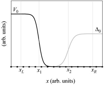
Figure 1: NS junction of an infinite nanowire. The black curve is the potential $V(x)$ created by a gate in contact with the nanowire while the gray curve is the superconductor gap induced by proximity with an s-wave superconductor. The normal contact ($x<x_{L}$) is characterized by potential $V_{0}$ and the superconductor one ($x>x_{R}$) by a gap $\Delta_{0}$. A smooth variation of $V(x)$ and $\Delta(x)$ occurs at transition points $x_{1}$ and $x_{2}$, respectively. A Zeeman magnetic field is applied homogenously along the entire nanowire pointing in $x$-direction while the Rashba SOI effective magnetic field points perpendicularly in $y$-direction. The numerical method uses a grid as indicated schematically by the dots on the $x$ axis.

The transitions between bulk values in $V(x)$ and $\Delta(x)$ are modeled with two soft Fermi functions centered at $x_{1}$ and $x_{2}$, respectively. Their softness is controlled with parameters $s_{1}$ and $s_{2}$. A zero softness means a step interface, while a high value implies a smooth one. These two functions read

$$V(x) = \frac{V_{0}}{1+e^{(x-x_{1})/s_{1}}}\;,$$ (2)

$$\Delta(x) = \Delta_{0}\left(1-\frac{1}{1+e^{(x-x_{2})/s_{2}}}\right)\;.$$ (3)

III Numerical method

The energy eigenstates fulfill the time independent Schrödinger equation with the Bolgoliubov-deGennes Hamiltonian,

$$\left(\mathcal{H}_{BdG}-E\right)\,\Psi(x,\eta_{\sigma},\eta_{\tau})=0\;,$$ (4)

where the wave function variables are the spatial coordinate $x\in(-\infty,\infty)$, the spin $\eta_{\sigma}\in\{\uparrow,\downarrow\}$ and the isospin $\eta_{\tau}\in\{\Uparrow,\Downarrow\}$. The basis projection for spin and isospin is taken in $\hat{z}$ orientation, with isospin up and down representing electron and hole quasiparticles, respectively. We expand next the wave function in spin and isospin spinors

$$\Psi(x,\eta_{\sigma},\eta_{\tau})=\sum_{s_{\sigma}s_{\tau}}{\Psi_{s_{\sigma}s_{\tau}}(x)\,\chi_{s_{\sigma}}(\eta_{\sigma})\,\chi_{s_{\tau}}(\eta_{\tau})}\;,$$ (5)

with the quantum numbers $s_{\sigma}=\pm$ and $s_{\tau}=\pm$. The spin and isospin states fulfill

$$\vec{\sigma}\cdot\hat{n}\,\chi_{s_{\sigma}}(\eta_{\sigma}) = s_{\sigma}\chi_{s_{\sigma}}(\eta_{\sigma})\,,$$ (6)

$$\tau_{z}\,\chi_{s_{\sigma}}(\eta_{\sigma}) = s_{\tau}\chi_{s_{\tau}}(\eta_{\tau})\,.$$ (7)

We numerically obtain the wave function amplitudes $\Psi_{s_{\sigma}s_{\tau}}(x)$ on the set of $N$ grid points, qualitatively sketched in Fig. 1 ($N$ is actually much larger than shown in the figure). In our approach, the energy $E$ is given and we determine whether a physical solution exists or not for that energy. In particular, MZM’s will be found for values of $E$ equal to zero. Using $n$-point finite difference formulas for the $x$-derivatives, Eq. (4) transforms on the grid into a matrix linear equation of homogenous type.

The solution must be compatible with the bulk boundary conditions for grid points in the normal $(x<x_{L})$ and superconductor contacts $(x>x_{R})$. In these asymptotic regions the solutions, at the desired energy $E$, are given by a linear combination of bulk eigensolutions $\Phi_{k}^{(c)}(x,\eta_{\sigma},\eta_{\tau})$, each one characterized by a wave number $k$ and $c=L,R$ being a generic label for the contact,

$$\Psi(x,\eta_{\sigma},\eta_{\tau})=\sum_{k}{C_{k}^{(c)}\,\Phi_{k}^{(c)}(x,\eta_{\sigma},\eta_{\tau})}\,.$$ (8)

The bulk eigensolutions are expressed in terms of exponentials

$$\Phi_{k}^{(c)}(x,\eta_{\sigma},\eta_{\tau})=\sum_{s_{\sigma}s_{\tau}}{\Phi_{ks_{\sigma}s_{\tau}}^{(c)}e^{ik(x-x_{c})}\chi_{s_{\sigma}}(\eta_{\sigma})\chi_{s_{\tau}}(\eta_{\tau})}\,.$$ (9)

The set of wave numbers and state coefficients $\{k,\Phi_{ks_{\sigma}s_{\tau}}^{(c)}\}$ characterizing the solutions in contact $c$ must be known in advance in order to proceed with the numerical calculations. These coefficients can be obtained for the homogenous and infinite problem either analytically or by means of additional numerical methods.Oreg et al. (2010); Serra (2013) Equation (8) must be fulfilled in replacement of Eq. (4) for grid points in the asymptotic regions. Notice that they are local relations in $x$ and, therefore, do not involve wave function amplitudes on points located further to the left or right of the grid ends.

Due to symmetries, there are always four bulk wave numbers per contact in outward direction. By outward direction we mean either exponentially decaying from the junction, in case of evanescent modes, or moving away from it in case of propagating modes. Notice that for propagating modes the flux direction is parallel and antiparallel to the corresponding real $k$ for quasiparticles of electron and hole type, respectively. A closed linear system for the set of $4N+4+4$ unknowns $\{\Psi_{s_{\sigma}s_{\tau}}(x),C^{(L)}_{k},C^{(R)}_{k}\}$ is easily obtained from Eqs. (4) and (8). A final complication, however, is found in the homogenous character of this linear system mathematically admitting the trivial solution of all unknowns equal to zero.

We discard the trivial solution by introducing an arbitrary matching point $x_{m}$ as well as a specific pair of spin-isospin components $(s,t)$. Assuming $\Psi_{st}(x_{m})$ does not identically vanish we can arbitrarily impose

$$\Psi_{st}(x_{m}) = 1\;,$$ (10)

$$\!\!\!\!\!\!\!\!\!\!\!\left(\frac{d^{(L)}}{dx}-\frac{d^{(R)}}{dx}\right)\Psi_{s_{\sigma}s_{\tau}}(x_{m}) = 0\;,\quad(s_{\sigma},s_{\tau})\neq(s,t)\,.$$ (11)

Equations (10) and (11) are four equations that we require at $x_{m}$ in place of the Bogoliubov-deGennes one. Thanks to Eq. (10) the resulting system is no longer homogenous. In Eq. (11), $d^{(L)}/dx$ and $d^{(R)}/dx$ indicate grid derivatives using only left or right grid neighbors. Crossing the matching point is actually avoided using non centered finite difference formulas. With this substitution of one equation the resulting linear system admits a nontrivial solution, robust with respect to changes in the arbitrary choices: $x_{m}$, $(s,t)$.

By means of Eq. (11) our algorithm ensures the continuity at the matching point of the first derivative for all spin-isospin components, with the exception of the arbitrarily chosen $(s,t)$. This relaxation of one condition makes the algorithm numerically robust and free from singularities. The mathematical solutions can be discriminated by defining the physical measure

$$\mathcal{F}=\left|\left(\frac{d^{(L)}}{dx}-\frac{d^{(R)}}{dx}\right)\Psi_{st}(x_{m})\right|^{2}\,.$$ (12)

Only those results with ${\cal F}=0$ are true physical solutions but this can be tested afterwards, at the end of the algorithm. Varying the energy $E$ or the Hamiltonian parameters the method allows the exploration of the topological phases.

The resulting system of equation is solved with a sparse-matrix linear algebra package.Har As in Refs. Oreg et al., 2010 and Serra, 2013 the numerical algorithm works in adimensional units, using the Rashba spin-orbit interaction (SOI) as a reference. The corresponding length and energy units read

$$L_{\it so} = \frac{\hbar^{2}}{\alpha m}\,,$$ (13)

$$E_{\it so} = \frac{\alpha^{2}m}{\hbar^{2}}\,.$$ (14)

IV Results without input flux

We study first the physics of the junction in absence of any input fluxes. Physically, this situation occurs when propagating modes in both contacts are either not active or, at most, they carry flux only in outwards direction from the junction. This behavior is expected in presence of purely absorbing (reflectionless) contacts. It is well known that in absence of propagating modes bounded MZM’s may exist in some cases. The allowed asymptotic wave numbers have an imaginary component causing the wave functions to decay away from the junction. As a consequence the main characteristic of these bounded MZM’s is that they are confined in a particular region of space. We will first check our method comparing with the analytical limits of Klinovaja and Loss,Klinovaja and Loss (2012) extending later the analysis to other results not obtainable analytically. These results range from the formation of Majorana modes in soft edge junctions of different kinds, to the influence of the edge on the MZM localization and protection.

IV.1 Comparison with analytical expressions

Reference Klinovaja and Loss, 2012 provides analytical expressions for MZM’s in a sharp NS junction, in a semi-infinite system. They are approximations valid deep into the topological phase $\Delta_{B}\gg\sqrt{\Delta_{o}^{2}+\mu^{2}}$. The approximations are done for both strong SOI ($E_{so}>>\Delta_{B}$) and weak SOI ($E_{so}<<\Delta_{B}$) regimes. In the strong SOI regime the Rashba spin orbit effect is the dominating term while the magnetic field and the superconductivity are treated as small perturbations. On the other hand, in the weak SOI regime the magnetic field term dominates. In Fig. 2 density distributions for NS junctions in a semi-infinite nanowire are shown for the strong and weak SOI regimes, as well as for an intermediate situation. The strong and weak regime numerical solutions (in dark-blue) are compared with their analytical counterparts (in light-green). The exclusion effect on the hard edge on the left is achieved in the numerical method by putting a very high sharp potential step at $x=-L$, while the sharp superconductor interface is located at $x=0$.

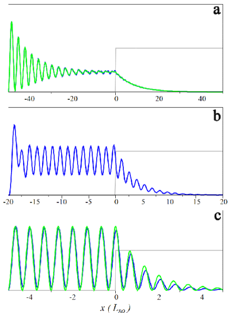
Figure 2: (Color online) Density distributions of MZM’s obtained with our numerical method (dark gray or blue) and with analytical approximations (light gray or green).Klinovaja and Loss (2012) a) Strong SOI regime $E_{so}>>\Delta_{B}$: $\Delta_{B}=0.09E_{so}$, $\Delta_{0}=0.06E_{so}$ and $L=50L_{so}$. b) Intermediate regime $E_{so}=\Delta_{B}$: $\Delta_{0}=0.2E_{so}$, $L=20L_{so}$. In this case the analytical result is not known. c) Weak SOI regime $E_{so}<<\Delta_{B}$: $\Delta_{B}=10E_{so}$, $\Delta_{0}=4E_{so}$ and $L=5L_{so}$.

The strong SOI Majorana density function is characterized by the combination of an oscillatory behavior modulated by exponential bounds in the normal side of the junction while, on the other hand, the weak SOI density is characterized by constant oscillations up to the NS interface. Entering the superconductor contact both densities decay, although in a more oscillatory way for the weak SOI. Note also that the intermediate regime $E_{so}\approx\Delta_{B}$ represents a sort of mixed situation with a first density peak near the $x=-L$ edge followed by regular oscillations of constant amplitude up to the NS junction. The theoretical and numerical results agree well in their corresponding regimes (but for some fine effects). However, the analytical solutions are not applicable out of their regimes of approximation. Therefore a numerical approach is potentially very useful in order to predict MZM’s density distributions in many realistic physical realizations that can be out of the strong and weak regimes in a varying degree.

IV.2 Soft edge junction results

Assume now the normal side contains a soft potential step characterized by a finite $V_{0}$, allowing some penetration. As can be seen in Fig. 3, this implies the appearance of a maximum in the density distribution near the potential edge followed by regular oscillations of decreasing amplitude. The density starts decaying exponentially in the superconductor interface until it vanishes well inside the superconductor side of the system.

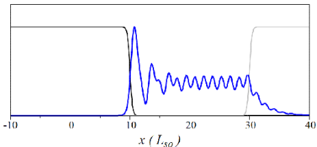
Figure 3: (Color online) MZM density (thick curve) in arbitrary scale when the potential interface is located at $x_{1}=10L_{so}$ with a softness parameter $s_{1}=0.2L_{so}$ and the superconductor gap interface is located at $x_{2}=30L_{so}$ with softness $s_{2}=0.2L_{so}$. The rest of parameters are $V_{o}=2E_{so}$, $\Delta_{o}=0.25E_{so}$, $\Delta_{B}=0.4E_{so}$ and $\mu=0.1E_{so}$. The position dependent potential and superconductor gap are shown by the thin black and gray curves, respectively.

The present method allows us to obtain the solutions not only for $E=0$ but for any arbitrary value of $E$. Figure 4 shows the location of the eigenstates in a $\Delta_{B}$-$E$ plane. They are signaled by the zeros of the function $\mathcal{F}$ [cf. Eq. (12)], represented here in a color (gray scale) plot. Black and white curves in Fig. 4 inform us on the presence of propagating modes in the superconductor and normal sides, respectively. That is, for energies above the curve propagating modes are possible in the superconductor (black) and normal (white) contacts. When propagating modes become possible asymptotically, the zeros of $\mathcal{F}$ no longer represent bounded states, but purely outgoing resonances created by the junction. In this case there is no violation of charge conservation since outgoing electron and hole equal fluxes imply zero currents.

For Zeeman energies lower than the critical value $\Delta_{B}^{(c)}\equiv\sqrt{\Delta_{0}^{2}+\mu^{2}}$ no MZM exists but, instead, finite energy subgap fermions may be found. Only those at positive energies are shown in Fig. 4, but the spectrum is exactly symmetrical for negative energies. When the magnetic field energy equals $\Delta_{B}^{(c)}$ the gap closes in the superconductor side. This is hinted in Fig. 4 by the presence of propagating modes in the superconductor side of the junction even at zero energies for this specific magnetic field. For higher fields the gap immediately reopens in the supercoductor region and the junction enters the topological phase with an $E=0$ solution, a MZM. In this phase finite energy resonant Andreev states can be found as well. The energy difference between the MZM and the finite energy states is a measure of the protection of the MZM. The greater the energy difference the greater the protection of the Majorana. Increasing further the magnetic field the MZM is finally destroyed due to the closing of the gap in the normal side of the junction. This is signaled by the appearance of propagating modes in this side of the junction even at zero energy. When the state at zero energy becomes propagating the bounded Majorana zero modes can not exist. All these results are in agreement with the present knowledge on MZM’s and represent a further check on our numerical method.

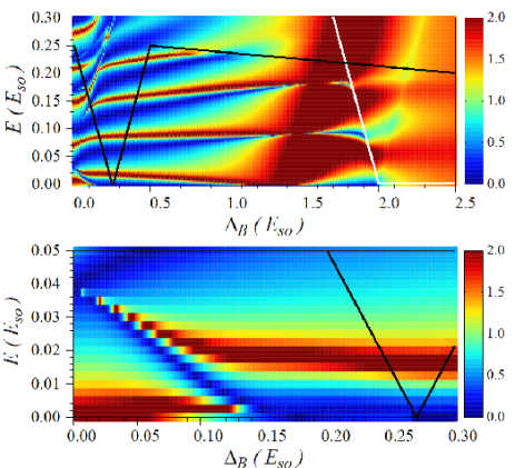
Figure 4: (Color online) a) Junction spectrum for different values of the magnetic field. The same parameters of Fig. 3 have been used. The colors represent the values of the function $\mathcal{F}$. Note that a solution exists when $\mathcal{F}=0$ (in dark-blue). Above the black line propagating modes exist in the superconductor side of the junction while above the white line the propagating modes exist in the normal side. b) Zoom of the spectrum showing the formation of the Majorana zero mode when the magnetic field becomes high enough for the system to perform a transition to the topological phase. $\Delta_{B}=0.27E_{so}$ is the topological critical value of the Zeeman field.

IV.3 Softness effects

This section is devoted to study the effects that changes in the softness parameter of the potential and superconductor interfaces cause on the Majorana density function and on the junction spectrum. In general, the shape of the density function is robust to moderate changes in the softness of the superconductor gap interface (see Fig. 5a). If we replace the sharp superconductor interface by a region of a gradually increasing superconductivity the Majorana wave function is not greatly affected. However, if we assume a very soft (almost linear) increase in superconductivity it is possible to see how the density tail of the MZM adapts to the appearance of the superconductivity (see Fig. 5b).

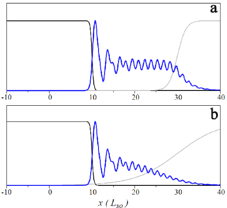
Figure 5: (Color online) a) Same as in Fig. 3 but with a softer superconductivity interface $s_{2}=L_{so}$. b) Same as in Fig. 2 and a) but with an even softer, almost linear, superconductivity interface $s_{2}=5L_{so}$.

The MZM is also robust with changes of the potential interface softness (see Fig. 6a). Again, only with an almost linear decrease of the junction potential a sizeable reduction of the density tail towards the supercoductor side can be seen with respect to the result for an abrupt potential. We also notice a slight increase in the width of the density peak as well as a change in the peak position (see Fig. 6b). Combining the two effects, if the softness of both potential and superconducting interfaces is high enough a MZM with a well localized density peak is found (see Fig. 8a).

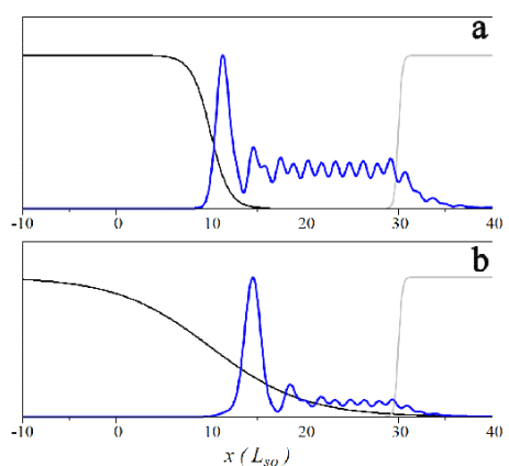
Figure 6: (Color online) a) Same as in Fig. 3 but with a potential softness parameter $s_{1}=L_{so}$ while the superconductor gap interface has a softness parameter $s_{2}=0.2L_{so}$. b) Same as a) but with a potential softness parameter $s_{1}=5L_{so}$.

A similar robustness against softness is found in the junction energy spectrum. Figure 7a shows the spectrum of eigenenergies, containing the MZM at zero energy and its closest excited bound and resonant states at finite energies. As before, the location of the eigenenergies is signaled by the zeros of the function $\mathcal{F}$ (in black). Note that although the function $\mathcal{F}$ is not symmetrical with respect to $E=0$, the position of the zeros indeed is. The particular shape of $\mathcal{F}$ is actually irrelevant and only the position of its zeros bears a physical meaning. The blue staircase curve informs us about the number of propagating modes in the superconductor side of the junction. The protection of the MZM, proportional to the energy gap with its nearby eigenenergies, does not change significantly for moderate values of the softness of the superconductor and potential interfaces. On the other hand, for high enough values of the softness interesting results arise.

For high values of the superconductor interface softness, shown in Fig. 7b, the protection of the MZM is increased since its neighboring eigenenergies are repelled from zero. In this case, the finite energy modes get closer to the activation energy of the propagating modes, i.e., to the energy gap on the superconductor side of the junction. On the contrary, the increase of the potential softness introduces more excited states inside the superconductor energy gap, thus getting closer to the MZM energy (see Fig. 7c). The appearance of low energy states in a soft potential interface is in agreement with the results of Ref. Kells et al., 2012. The characteristic features of these low energy states in tunneling conductance experiments were discussed in Ref. Stanescu and Tewari, 2013b.

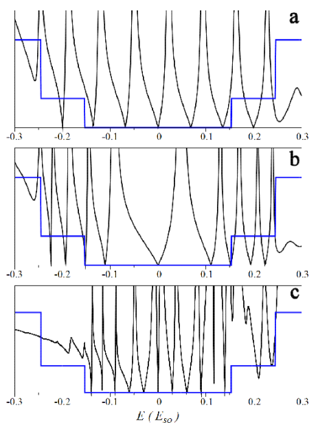
Figure 7: (Color online) a) Junction spectrum when the potential interface is located at $x_{1}=10L_{so}$ while the superconductor gap interface is located at $x_{2}=30L_{so}$ both with softness parameters $s_{1}=s_{2}=0.2L_{so}$. The rest of parameters are $V_{0}=2E_{so}$, $\Delta_{o}=0.25E_{so}$, $\Delta_{B}=0.4E_{so}$ and $\mu=0$. The function $\mathcal{F}$ is shown in black while the number of propagating modes in the superconductor side of the junction is shown in blue-gray. Each step corresponds to the activation of a propagating mode. The zeros of $\mathcal{F}$ indicate the existence of a solution with the corresponding energy $E$. b) Same as a) but with a superconductor gap interface softness $s_{2}=10L_{so}$ while the potential softness is $s_{1}=0.2L_{so}$. c) same as a) and b) but this time with a potential interface softness $s_{1}=10L_{so}$ and a superconductor gap interface softness $s_{2}=0.2L_{so}$.

When both interfaces are made soft the two effects on the spectrum we have just discussed compete. That is, the higher softness of the potential introduces more bound states inside the superconductor energy gap, while the softness of the superconducting interface tries to push them apart from the MZM. The result is that many excited states get densely packed near the superconducting gap energy (see Fig. 8b).

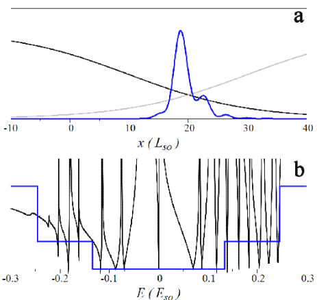
Figure 8: (Color online) a) MZM density when the potential interface is located at $x_{1}=10L_{so}$ while the superconductor interface is located at $x_{2}=30L_{so}$, both with a softness parameter $s_{1}=s_{2}=10L_{so}$. The rest of parameters are $V_{o}=2E_{so}$, $\Delta_{o}=0.25E_{so}$, $\Delta_{B}=0.4E_{so}$ and $\mu=0.1E_{so}$. b) Energy spectrum of the junction in a). As before the function $\mathcal{F}$ is shown in black while the number of propagating modes in the superconductor side of the junction is shown in blue-gray. Zeros in $\mathcal{F}$ indicate the existence of a solution with the corresponding energy $E$.

IV.4 MZM’s in different kinds of junctions

Up to this point it has been assumed that the position of the potential interface $x_{1}$ and the superconduction interface $x_{2}$ are such that $x_{1}<x_{2}$, i.e., they do not overlap. In this subsection we consider a more general situation, defining two kind of junctions: type I junctions without overlapping region ($x_{1}<x_{2}$) and type II junctions in the opposite case ($x_{1}>x_{2}$). Figure 9 shows a comparison between both types, as well as the limiting intermediate situation. In type I junctions the MZM density behaves as in previous sections, with a density peak localized on the potential edge followed by regular oscillations and a decaying behavior inside the superconductor region. On the other hand, type II junctions just show an oscillatory density whose amplitude decays as the function penetrates the superconductor region. The limiting case $x_{1}=x_{2}$ behaves similarly to the type II junction.

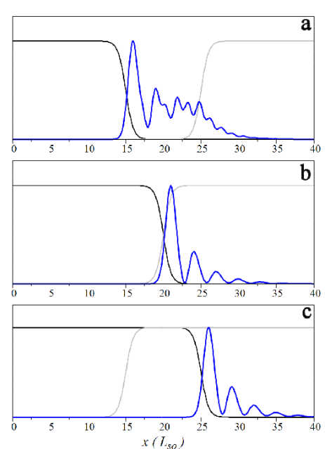
Figure 9: (Color online) Different kinds of soft NS junctions in an infinite nanowire. The used parameters are $V_{o}=2E_{so}$, $\Delta_{o}=0.25E_{so}$, $\Delta_{B}=0.4E_{so}$ and $\mu=0.1E_{so}$. Panel a) is for a type I junction, with non overlapping high potential and superconductivity regions. Panel c), for a type II junction, is just the opposite. Panel b) is the limiting case between the two when the potential and superconductor interfaces are located at the same point.

We also notice from Fig. 9 that the density peak is always found close to the potential interface. That is, the MZM is located on the potential step and not on the superconductivity interface. Superconductivity is a necessary ingredient for the formation of the MZM but, in practice, its maximum probability can be located quite far from the superconductor interface.

As shown in Fig. 7a, bounded states are found in type I junctions at energies different from zero. We believe these states are Andreev resonant states formed in the region between the two interfaces. This statement is confirmed by means of a change in the superconductor bulk value $\Delta_{0}$. As shown in Fig. 10, out of the topological regime the MZM splits into two subgap Fermionic states but the Andreev resonant states remain almost with the same eigenenergies. Notice also that the number of Andreev states is larger and their energies are closer to zero in type I junctions with a large non overlapping region, i.e., large $d=x_{2}-x_{1}$ (see Fig. 11a). On the contrary, if $d$ is diminished the number of Andreev resonant states diminishes an their energies fall apart from zero. In the limiting case when $d$ is zero the Andreev resonant states disappear and the protection of the MZM is determined by the amplitude of the gap on the superconductor side of the junction as shown in Fig 11b. The same happens for type II junctions with $d<0$. Furthermore, in this case ($d\leq 0$) the junction spectrum is even more resilient to changes in the softness of the interfaces, being almost insensitive to them.

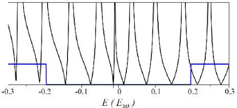
Figure 10: (Color online) Junction spectrum out of the topological phase. In this regime the MZM is split into two subgap fermions. The used parameters are $V_{o}=2E_{so}$, $\Delta_{o}=0.6E_{so}$, $\Delta_{B}=0.4E_{so}$ and $\mu=0$.

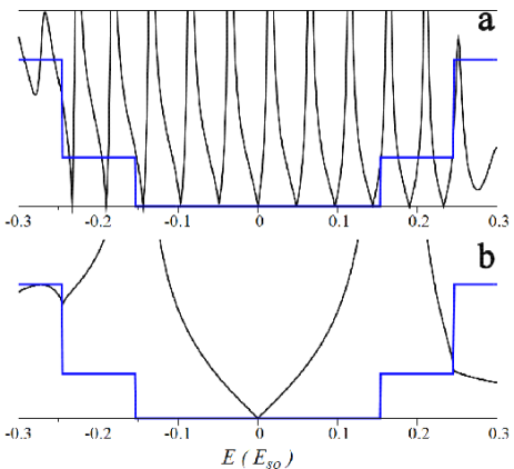
Figure 11: (Color online) Spectra for different kinds of junctions. The used parameters are $V_{o}=2E_{so}$, $\Delta_{o}=0.25E_{so}$, $\Delta_{B}=0.4E_{so}$ and $\mu=0$. Panel a) is for a type I junction with a long separation between potential and superconductor interfaces ($d=30L_{so}$) while panel b) corresponds to the limiting case between type I and type II junctions when both interfaces are located on the same position ($d=0$). Like in preceding figures the zeros of $\mathcal{F}$ indicate the existence of a solution with the corresponding energy $E$.

V Results with input flux

Decreasing the potential $V_{0}$, for a fixed $\Delta_{B}$, $\Delta_{0}$, and zero energy, wave functions characterized by real wave numbers arise in the bulk normal side of the junction. When this occurs, bounded MZM’s no longer exist due to their coupling with propagating modes. In the preceding section we assumed that if propagating modes were present they only carried outgoing flux. In this section we explore the influence of incident fluxes on the junction. The same numerical method explained above can be used here, disregarding the use of the matching point and just fixing the coefficients $C_{k}$ of the input modes as this already yields a non homogenous linear system. We only consider input modes from the normal side of the junction, given by electron states of positive $k$ and hole states of negative $k$. Furthermore, it is also assumed that all propagating input modes impinge on the junction with exactly the same flux.

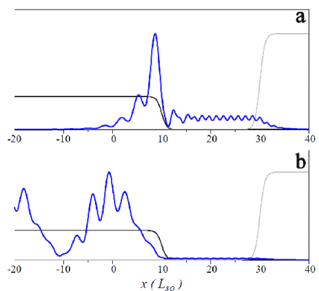
Figure 12: (Color online) a) Majorana bounded state found for $V_{o}=0.69E_{so}$, $\Delta_{o}=0.25E_{so}$, $\Delta_{B}=0.4E_{so}$ and $\mu=0.1E_{so}$. Potential and superconductor interfaces are located at $x_{1}=10L_{so}$ and $x_{2}=30L_{so}$ respectively and their softness parameters are $s_{1}=s_{2}=0.5L_{so}$. b) Zero energy non Majorana extended state. The figure is shown for the same parameters as in a) but with $V_{0}=0.67E_{so}$.

Following the sequence from high to low values of $V_{0}$, the system evolves from no propagating modes at high $V_{0}$ to four input modes (with two different $k$’s) for moderately low values of the potential $V_{0}$. In this case, the resulting zero mode density is characterized by a beating pattern of a large wave length modulated by a smaller one (see Fig. 12b). For $\Delta_{0}=0.25E_{so}$ and $\Delta_{B}=0.4E_{so}$ this regime ranges from $V_{0}=0.68E_{so}$, where the propagating modes arise, down to $V_{0}=0.50E_{so}$. Above $V_{0}=0.68E_{so}$ only evanescent modes are possible (see Fig. 12a). The zero mode solution obtained in this range does not represent a MZM since its wave function components do not fulfill the requirement

$$\Psi_{s_{\sigma}s_{\tau}}(x)=(-1)^{\frac{s_{\sigma}-s_{\tau}}{2}}\,\Psi_{-s_{\sigma}-s_{\tau}}^{*}(x)\;.$$ (15)

For $V_{0}<0.50E_{so}$ half of the normal side allowed wave numbers become purely imaginary, thus leading to an evanescent contribution to the boundary condition. As a consequence, there are only two modes (with the same $k$) and the resulting density has a single period of oscillation (see Fig. 13b). In this case the wave function represents a MZM since it fulfills Eq. (15). This example of extended MZM’s demonstrates that their existence is not limited to bounded states. For these extended states the assumption of equal incident flux in electron and hole channels is crucial. If the input is prepared in a specific electron or hole state of a given spin, the MZM condition Eq. (15) is lost for low values of the bulk potential. Therefore, propagating MZM’s are possible albeit for a particular superposition of input states only.

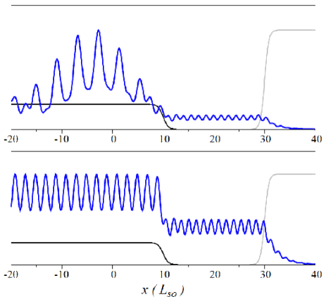
Figure 13: (Color online) a) Non Majorana bounded state found for $V_{0}=0.51E_{so}$, $\Delta_{o}=0.25E_{so}$, $\Delta_{B}=0.4E_{so}$ and $\mu=0.1E_{so}$. Excluding $V_{0}$ these are the same parameters as in Figs. 12a and 12b. b) Density for a MZM extended state. The figure is shown for the same parameters as in a) but with $V_{0}=0.49E_{so}$.

VI Conclusions

A numerical method to calculate the wave function of MZM’s in presence of a soft normal-superconductor junction has been developed. This method is able to detect whether a particular energy $E$ is an eigenenergy or not of the junction and, when it is the case, obtain the corresponding wave function. The junction is described by smooth functions of position in a 1D nanowire with Rashba spin orbit interaction, a Zeeman magnetic field and superconductivity. It has been applied to a semi-infinite abrupt nanowire junction in order to compare its results with those obtained analytically, as well as to infinite soft junctions in order to study the dependence to different parameters of the MZM density and its protection from energetically alike excited states.

We have proven the resilience of the MZM density to the softness parameters and studied the dependence of its localization with the potential interface position. This latter feature hints the possibility of manipulating the position of the Majorana modes in order to perform topological quantum operations. We have found the remarkable result of an increase in the protection of the MZM for high values of the softness of the superconductor gap interface, while high values of the softness of the potential interface have an opposite effect. Finally, we have shown the existence of extended MZM’s, albeit limited to feed the junction with a particular set of propagating input states. This result demonstrates that MZM’s are not always restricted to bounded states.