A Multivariate Functional Limit Theorem in Weak $M_{1}$ Topology

Abstract

We show a new functional limit theorem for weakly dependent regularly varying sequences of random vectors. As it turns out, the convergence takes place in the space of $\mathbb{R}^{d}$ valued càdlàg functions endowed with the so-called weak $M_{1}$ topology. The theory is illustrated on two examples. In particular, we demonstrate why such an extension of Skorohod’s $M_{1}$ topology is actually necessary for the limit theorem to hold.

1 Introduction

Literature in theoretical probability and statistics abounds with studies of the limiting behaviour of partials sums, mostly in the case of stationary sequences with so-called light tails. On the other hand, many applied probabilistic models, in teletraffic and insurance modelling for instance, frequently produce distributions with heavy tails and even infinite variance. Regularly varying distributions underlying some of these models fit various data sets particularly well (see Embrechts et al. [14] for examples of financial/actuarial data fitting such a hypothesis).

We consider a stationary sequence of $\mathbb{R}^{d}$ valued random vectors $(X_{n})_{n\geqslant 1}$ and its accompanying sequence of partial sums $S_{n}=X_{1}+\cdots+X_{n},\ {n\geqslant 1}$. If the $X_{n}$ are i.i.d. and regularly varying with index $\alpha\in(0,2)$, then

$$\frac{S_{n}-b_{n}^{\prime}}{a_{n}^{\prime}}\xrightarrow{d}S_{\alpha}\quad\textrm{in}\ \mathbb{R}^{d},$$ (1.1)

for some sequences $a_{n}^{\prime}>0$ and $b_{n}^{\prime}$ and some non-degenerate $\alpha$–stable random vector $S_{\alpha}$, see Rvačeva [27] (the univariate result goes back to Gnedenko and Kolmogorov). Weakly dependent sequences, satisfying strong mixing condition for instance, can exhibit a very similar behavior. From the large literature on this phenomenon we refer here to Durrett and Resnick [13], Davis [9], Denker and Jakubowski [12], Avram and Taqqu [1], Davis and Hsing [10] and Bartkiewicz et al. [2] in the one-dimensional case, and Phillip [23], [24], Jakubowski and Kobus [17] and Davis and Mikosch [11] in the multi-dimensional case.

In this paper we are interested in the functional generalization of (1.1). For infinite variance i.i.d. regularly varying sequences $(X_{n})$ in the one-dimensional case functional limit theorem was established in Skorohod [29]. A very readable proof of this result in the multivariate case can be found in Resnick [26] using Skorohod’s $J_{1}$ topology on $D([0,1],\mathbb{R}^{d})$. Tyran-Kamińska [30] recently studied the problem for a more general class of weakly dependent stationary sequences using the same topology. However, this choice of topology excludes many processes used in applications. To study such models we are forced to use a weaker topology.

Our main theorem extends the main result in Basrak et al. [5] to the multivariate setting. In [5] a functional limit theorem has been obtained for stationary, regularly varying sequence of dependent random variables for which clusters of high-threshold excesses can be broken down into asymptotically independent blocks, using the Skorohod’s $M_{1}$ topology. Direct generalization of this result to random vectors fails in standard $M_{1}$ topology, as illustrated by an example in Section 4. It turns out that the limit theorem still holds but in the weak $M_{1}$ topology. This topology is strictly weaker than the standard $M_{1}$ topology on $D([0,1],\mathbb{R}^{d})$ for $d\geqslant 2$ (cf. Whitt [31]). Our main result seems to be the first generic functional limit theorem which holds in weak $M_{1}$ topology, but fails in other more frequently used topologies on $D([0,1],\mathbb{R}^{d})$.

2 Assumptions

2.1 Regular variation

Denote $\mathbb{E}=[-\infty,\infty]^{d}\setminus\{0\}$. The space $\mathbb{E}$ is equipped with the topology in which a set $B\subset\mathbb{E}$ has compact closure if and only if it is bounded away from zero, that is, if there exists $u>0$ such that $B\subset\mathbb{E}_{u}=\{x\in\mathbb{E}:\|x\|>u\}$. Denote by $C_{K}^{+}(\mathbb{E})$ the class of all nonnegative, continuous functions on $\mathbb{E}$ with compact support.

We say that a strictly stationary process $(X_{n})_{n\in\mathbb{Z}}$ is (jointly) regularly varying with index $\alpha\in(0,\infty)$ if for any nonnegative integer $k$ the $kd$-dimensional random vector $X=(X_{1},\ldots,X_{k})$ is multivariate regularly varying with index $\alpha$, i.e. there exists a random vector $\Theta$ on the unit sphere $\mathbb{S}^{kd-1}=\{x\in\mathbb{R}^{kd}:\|x\|=1\}$ such that for every $u\in(0,\infty)$ and as $x\to\infty$,

$$\frac{\operatorname{P}(\|X\|>ux,\,X/\|X\|\in\cdot\,)}{\operatorname{P}(\|X\|>x)}\xrightarrow{w}u^{-\alpha}\operatorname{P}(\Theta\in\cdot\,),$$ (2.1)

the arrow “$\xrightarrow{w}$” denoting weak convergence of finite measures.

Theorem 2.1 in Basrak and Segers [6] provides a convenient characterization of joint regular variation: it is necessary and sufficient that there exists a process $(Y_{n})_{n\in\mathbb{Z}}$ with $\operatorname{P}(\|Y_{0}\|>y)=y^{-\alpha}$ for $y\geqslant 1$ such that as $x\to\infty$,

$$\bigl{(}(x^{-1}\ X_{n})_{n\in\mathbb{Z}}\,\big{|}\,\|X_{0}\|>x\bigr{)}\xrightarrow{\text{fidi}}(Y_{n})_{n\in\mathbb{Z}},$$ (2.2)

where “$\xrightarrow{\text{fidi}}$” denotes convergence of finite-dimensional distributions. The process $(Y_{n})_{n\in\mathbb{Z}}$ is called the tail process of $(X_{n})_{n\in\mathbb{Z}}$. Writing $\Theta_{n}=Y_{n}/\|Y_{0}\|$ for $n\in\mathbb{Z}$, we also have

$$\bigl{(}(\|X_{0}\|^{-1}X_{n})_{n\in\mathbb{Z}}\,\big{|}\,\|X_{0}\|>x\bigr{)}\xrightarrow{\text{fidi}}(\Theta_{n})_{n\in\mathbb{Z}},$$ (2.3)

see Corollary 3.2 in [6]. The process $(\Theta_{n})_{n\in\mathbb{Z}}$ is independent of $\|Y_{0}\|$ and is called the spectral (tail) process of $(X_{n})_{n\in\mathbb{Z}}$. The law of $\Theta_{0}=Y_{0}/\|Y_{0}\|\in\mathbb{S}^{d-1}$ is the spectral measure of the common distribution of the random vectors $X_{i}$. Regular variation of this distribution can be expressed in terms of vague convergence of measures on $\mathbb{E}$ as follows: for $a_{n}$ as such that

$$n\operatorname{P}(\|X_{1}\|>a_{n})\to 1,$$ (2.4)

as $n\to\infty$,

$$n\operatorname{P}(a_{n}^{-1}X_{i}\in\cdot\,)\xrightarrow{v}\mu(\,\cdot\,),$$ (2.5)

where the limit $\mu$ is a nonzero Radon measure on $\mathbb{E}$ that satisfies $\mu([-\infty,\infty]^{d}\setminus\mathbb{R}^{d})=0$. Further, the measure $\mu$ satisfies the following scaling property

$$\mu(u\,\cdot\,)=u^{-\alpha}\mu(\,\cdot\,),$$ (2.6)

for every $u>0$, where $\alpha$ is the same sa in relation (2.1).

2.2 Point processes and dependence conditions

We define the time-space point processes

$$N_{n}=\sum_{i=1}^{n}\delta_{(i/n,\,X_{i}/a_{n})}\qquad\text{ for all $n\in\mathbb{N}$,}$$ (2.7)

with $a_{n}$ as in (2.4). In this section we find a limit in distribution for the sequence $(N_{n})_{n}$ in the state space $[0,1]\times\mathbb{E}_{u}$ for $u>0$ under appropriate dependence assumptions. The limit process is a Poisson superposition of cluster processes, whose distribution is determined by the law of the tail process $(Y_{i})_{i\in\mathbb{Z}}$.

To control the dependence in the sequence $(X_{n})_{n\in\mathbb{Z}}$ we first have to assume that clusters of large values of $\|X_{n}\|$ have finite mean size, roughly speaking.

Condition 2.1

There exists a positive integer sequence $(r_{n})_{n\in\mathbb{N}}$ such that $r_{n}\to\infty$ and $r_{n}/n\to 0$ as $n\to\infty$ and such that for every $u>0$,

$$\lim_{m\to\infty}\limsup_{n\to\infty}\operatorname{P}\biggl{(}\max_{m\leqslant|i|\leqslant r_{n}}\|X_{i}\|>ua_{n}\,\bigg{|}\,\|X_{0}\|>ua_{n}\biggr{)}=0.$$ (2.8)

Put $M_{1,n}=\max\{\|X_{i}\|:i=1,\ldots,n\}$ for $n\in\mathbb{N}$. In Proposition 4.2 in [6], it has been shown that under Condition 2.1 the following holds

$$\theta = \lim_{r\to\infty}\lim_{x\to\infty}\operatorname{P}\bigl{(}M_{1,r}\leqslant x\,\big{|}\,\|X_{0}\|>x\bigr{)}$$ (2.9)

$$= \operatorname{P}({\textstyle\sup_{i\geqslant 1}}\|Y_{i}\|\leqslant 1)=\operatorname{P}({\textstyle\sup_{i\leqslant-1}}\|Y_{i}\|\leqslant 1)>0.$$

By Remark 4.7 in [6], alternative expressions for $\theta$ in (2.9) are

$$\theta = \int_{1}^{\infty}\operatorname{P}\biggl{(}\sup_{i\geqslant 1}\|\Theta_{i}\|^{\alpha}\leqslant y^{-\alpha}\biggr{)}\,\mathrm{d}(-y^{-\alpha})$$

$$= \operatorname{E}\biggl{[}\max\biggl{(}1-\sup_{i\geqslant 1}\|\Theta_{i}\|^{\alpha},0\biggr{)}\biggr{]}=\operatorname{E}\biggl{[}\sup_{i\geqslant 0}\|\Theta_{i}\|^{\alpha}-\sup_{i\geqslant 1}\|\Theta_{i}\|^{\alpha}\biggr{]}.$$

Moreover we have $\operatorname{P}(\lim_{|n|\to\infty}\|Y_{n}\|=0)=1$. Also, for every $u\in(0,\infty)$

$$\operatorname{P}(M_{1,r_{n}}\leqslant a_{n}u\mid\|X_{0}\|>a_{n}u)=\frac{\operatorname{P}(M_{1,r_{n}}>a_{n}u)}{r_{n}\operatorname{P}(\|X_{0}\|>a_{n}u)}+o(1)\to\theta$$ (2.10)

as $n\to\infty$.

In the sequel, the point processes

$$\sum_{i=1}^{r_{n}}\delta_{(a_{n}u)^{-1}X_{i}}\quad\text{conditionally on}\quad M_{1,r_{n}}>a_{n}u\,,$$

are called cluster processes. We use them to describe a cluster of extremes occurring in a relatively short time span. Theorem 4.3 in [6] yields the weak convergence of the sequence of cluster processes in the state space $\mathbb{E}$:

$$\biggl{(}\sum_{i=1}^{r_{n}}\delta_{(a_{n}u)^{-1}X_{i}}\,\bigg{|}\,M_{1,r_{n}}>a_{n}u\biggr{)}\xrightarrow{d}\biggl{(}\sum_{j\in\mathbb{Z}}\delta_{Y_{j}}\,\bigg{|}\,\sup_{i\leqslant-1}\|Y_{i}\|\leqslant 1\biggr{)}.$$ (2.11)

Note that since $\|Y_{n}\|\to 0$ almost surely as $|n|\to\infty$, the point process $\sum_{n}\delta_{Y_{n}}$ is well-defined in $\mathbb{E}$. By (2.9), the probability of the conditioning event on the right-hand side of (2.11) is nonzero.

To establish convergence of $N_{n}$ in (2.7), we need to impose a certain mixing condition called $\mathcal{A}^{\prime}(a_{n})$ which is slightly stronger than the condition $\mathcal{A}(a_{n})$ introduced in Davis and Hsing [10] and Davis and Mikosch [11].

Condition 2.2 ($\mathcal{A}^{\prime}(a_{n})$)

There exists a sequence of positive integers $(r_{n})_{n}$ such that $r_{n}\to\infty$ and $r_{n}/n\to 0$ as $n\to\infty$ and such that for every $f\in C_{K}^{+}([0,1]\times\mathbb{E})$, denoting $k_{n}=\lfloor n/r_{n}\rfloor$, as $n\to\infty$,

$$\operatorname{E}\biggl{[}\exp\biggl{\{}-\sum_{i=1}^{n}f\biggl{(}\frac{i}{n},\frac{X_{i}}{a_{n}}\biggr{)}\biggr{\}}\biggr{]}-\prod_{k=1}^{k_{n}}\operatorname{E}\biggl{[}\exp\biggl{\{}-\sum_{i=1}^{r_{n}}f\biggl{(}\frac{kr_{n}}{n},\frac{X_{i}}{a_{n}}\biggr{)}\biggr{\}}\biggr{]}\to 0.$$ (2.12)

It can be shown that Condition 2.2 is implied by the strong mixing property, see Krizmanić [20].

The proof of Theorem 2.3 in Basrak et al. [5] carries over to the multivariate case with some straightforward adjustments. Hence, we obtain the following result describing exceedences in the sequence $(X_{n})$ outside of the ball of radius $u$ around the origin.

Theorem 2.3

Assume that Conditions 2.1 and 2.2 hold for the same sequence $(r_{n})$, then for every $u\in(0,\infty)$ and as $n\to\infty$,

$$N_{n}\bigg{|}_{[0,1]\times\mathbb{E}_{u}}\,\xrightarrow{d}N^{(u)}=\sum_{i}\sum_{j}\delta_{(T^{(u)}_{i},uZ_{ij})}\bigg{|}_{[0,1]\times\mathbb{E}_{u}}\,,$$

in $[0,1]\times\mathbb{E}_{u}$ and

1. $\sum_{i}\delta_{T^{(u)}_{i}}$ is a homogeneous Poisson process on $[0,1]$ with intensity $\theta u^{-\alpha}$,

2. $(\sum_{j}\delta_{Z_{ij}})_{i}$ is an i.i.d. sequence of point processes in $\mathbb{E}$, independent of $\sum_{i}\delta_{T^{(u)}_{i}}$, and with common distribution equal to the weak limit in (2.11).

3 Functional limit theorem

In the main result in the article, we show the convergence of the partial sum process $V_{n}$ to a stable Lévy process in the space $D([0,1],\mathbb{R}^{d})$ equipped with Skorohod’s weak $M_{1}$ topology. As in the one dimensional case (cf. Basrak et al. [5]) we first represent the partial sum process $V_{n}$ as the image of the time-space point process $N_{n}$ in (2.7) under a certain summation functional. Then, since this summation functional enjoys the right continuity properties, by an application of the continuous mapping theorem we transfer the weak convergence of $N_{n}$ in Theorem 2.3 to weak convergence of $V_{n}$.

3.1 The weak $M_{1}$ topology

For $a=(a^{1},\ldots,a^{d}),b=(b^{1},\ldots,b^{d})\in\mathbb{R}^{d}$, let $[[a,b]]$ be the product segment, i.e.

$$[[a,b]]=[a^{1},b^{1}]\times[a^{2},b^{2}]\times\dots\times[a^{d},b^{d}].$$

For $x\in D([0,1],\mathbb{R}^{d})$ the completed graph of $x$ is the set

$$G_{x}=\{(t,z)\in[0,1]\times\mathbb{R}^{d}:z\in[[x(t-),x(t)]]\},$$

where $x(t-)$ is the left limit of $x$ at $t$. We define an order on the graph $G_{x}$ by saying that $(t_{1},z_{1})\leqslant(t_{2},z_{2})$ if either (i) $t_{1}<t_{2}$ or (ii) $t_{1}=t_{2}$ and $|x^{j}(t_{1}-)-z^{j}_{1}|\leqslant|x^{j}(t_{2}-)-z^{j}_{2}|$ for all $j=1,\ldots,d$. Clearly, the relation $\leqslant$ induces only a partial order on the graph $G_{x}$. A weak parametric representation of the graph $G_{x}$ is a continuous nondecreasing function $(r,u)$ mapping $[0,1]$ into $G_{x}$, with $r\in C([0,1],[0,1])$ being the time component and $u=(u^{1},\ldots,u^{d})\in C([0,1],\mathbb{R}^{d})$ being the spatial component, such that $r(0)=0,r(1)=1$ and $u(1)=x(1)$. Let $\Pi_{w}(x)$ denote the set of weak parametric representations of the graph $G_{x}$. For $x_{1},x_{2}\in D([0,1],\mathbb{R}^{d})$ define

$$d_{w}(x_{1},x_{2})=\inf\{\|r_{1}-r_{2}\|_{[0,1]}\vee\|u_{1}-u_{2}\|_{[0,1]}:(r_{i},u_{i})\in\Pi_{w}(x_{i}),i=1,2\},$$

where $\|x\|_{[0,1]}=\sup\{\|x(t)\|:t\in[0,1]\}$. Now we say that $x_{n}\to x$ in $D([0,1],\mathbb{R}^{d})$ for a sequence $(x_{n})$ in the weak Skorohod’s $M_{1}$ (or shortly $WM_{1}$) topology if $d_{w}(x_{n},x)\to 0$ as $n\to\infty$. The $WM_{1}$ topology is weaker than the standard $M_{1}$ topology on $D([0,1],\mathbb{R}^{d})$. Note, however that for $d=1$ two topologies coincide. The $WM_{1}$ topology coincides with the topology induced by the metric

$$d_{p}(x_{1},x_{2})=\max\{d_{M_{1}}(x_{1}^{j},x_{2}^{j}):j=1,\ldots,d\}$$

for $x_{i}=(x_{i}^{1},\ldots,x_{i}^{d})\in D([0,1],\mathbb{R}^{d})$ and $i=1,2$ (here $d_{M_{1}}$ denotes the standard Skorohod’s $M_{1}$ metric on $D([0,1],\mathbb{R})$). The metric $d_{p}$ induces the product topology on $D([0,1],\mathbb{R}^{d})$. For detailed discussion of the weak $M_{1}$ topology we refer to Whitt [31].

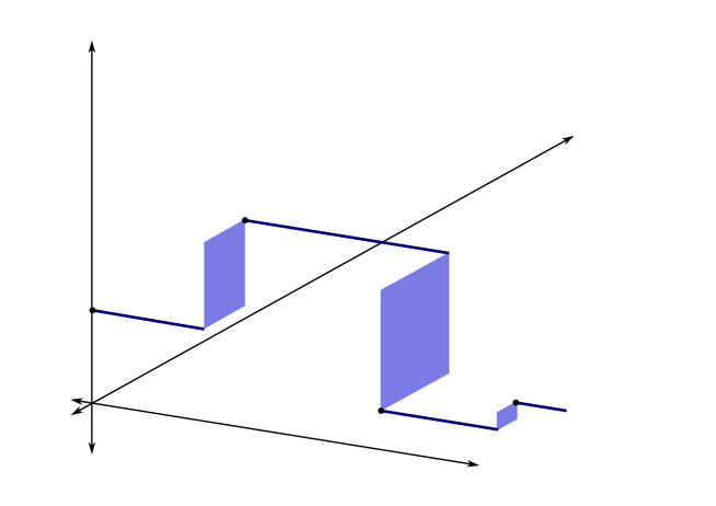
Figure 1: Completed graph of a cádlág function in $\mathbb{R}^{2}$.

3.2 Continuity of summation functional

Fix $0<v<u<\infty$. The proof of our main theorem depends on the continuity properties of the summation functional

$$\psi^{(u)}\colon\mathbf{M}_{p}([0,1]\times\mathbb{E}_{v})\to D([0,1],\mathbb{R}^{d})$$

defined by

$$\psi^{(u)}\bigl{(}{\textstyle\sum}_{i}\delta_{(t_{i},\,(x_{i}^{1},\ldots,x_{i}^{d}))}\bigr{)}(t)=\Big{(}\sum_{t_{i}\leqslant t}x_{i}^{j}\,1_{\{u<|x_{i}^{j}|<\infty\}}\Big{)}_{j=1,\ldots,d},\qquad t\in[0,1].$$

Observe that $\psi^{(u)}$ is well defined because $[0,1]\times\mathbb{E}_{u}$ is a relatively compact subset of $[0,1]\times\mathbb{E}_{v}$. The space $\mathbf{M}_{p}$ of Radon point measures is equipped with the vague topology and $D([0,1],\mathbb{R}^{d})$ is equipped with the weak $M_{1}$ topology.

We will show that $\psi^{(u)}$ is continuous on the set $\Lambda=\Lambda_{1}\cap\Lambda_{2}$, where

$$\Lambda_{1}=\{\eta\in\mathbf{M}_{p}([0,1]\times\mathbb{E}_{v}):\eta(\{0,1\}\times\mathbb{E}_{u})=0\ \textrm{and}\\[3.00003pt] \eta([0,1]\times\{x=(x^{1},\ldots,x^{d}):|x^{i}|\in\{u,\infty\}\ \textrm{for some}\ i\})=0\},\\[10.00002pt] \Lambda_{2}=\{\eta\in\mathbf{M}_{p}([0,1]\times\mathbb{E}_{v}):\text{for all $t\in[0,1]$},\ \eta(\{t\}\times\prod_{j=1}^{d}A_{j})=0\ \textrm{for all except}\\[3.00003pt] \textrm{at most one set}\ \prod_{j=1}^{d}A_{j}\ \textrm{where}\ A_{j}=(0,+\infty]\ \textrm{or}\ A_{j}=[-\infty,0)\}.$$

Lemma 3.1

Assume that with probability one, the tail process $(Y_{i})_{i\in\mathbb{Z}}$ in (2.2) satisfies the property that for every $j=1,\ldots,d$, $(Y_{i}^{j})_{i\in\mathbb{Z}}$ has no two values of the opposite sign. Then $\operatorname{P}(N^{(v)}\in\Lambda)=1$.

Proof 1

Recall that we can write $Y_{i}^{j}=\|Y_{0}\|\,\Theta_{i}^{j}$ for all indices $i$ and coordinates $j$, see (2.3). Observe that random variable $\|Y_{0}\|$ is continuous and independent of all $\Theta_{i}^{j}$’s to obtain

$$\operatorname{P}(|Y_{i}^{j}|=u/v\ \textrm{for some}\ j=1,\ldots,d)=0.$$

Therefore, in light of Theorem 2.3 it holds that

$$\operatorname{P}\Big{(}\sum_{j}\delta_{vZ_{ij}}(\{x=(x^{1},\ldots,x^{d}):|x^{k}|=u\ \textrm{for some}\ k\})=0\Big{)}$$

$$= \operatorname{P}\Big{(}\sum_{j}\delta_{Z_{ij}}(\{x:|x^{k}|=u/v\ \textrm{for some}\ k\}\Big{)}=0)$$

$$= \operatorname{P}\Big{(}\sum_{j}\delta_{Y_{j}}(\{x=(x^{1},\ldots,x^{d}):|x^{k}|=u/v\ \textrm{for some}\ k\})=0\,\Big{|}\,\sup_{i}\|Y_{i}\|\leqslant-1\Big{)}$$

$$= 1.$$

Hence

$$\operatorname{P}(N^{v}([0,1]\times\{x=(x^{1},\ldots,x^{d}):|x^{k}|=u\ \textrm{for some}\ k\})=0)=1.$$

We obtain the same result if above we replace $u$ by $+\infty$, and this together with the fact that $\operatorname{P}(\sum_{i}\delta_{T_{i}^{(v)}}(\{0,1\})=0)=1$ implies $\operatorname{P}(N^{(v)}\in\Lambda_{1})=1$.

Second, the assumption that with probability one $(Y_{i}^{j})_{i\in\mathbb{Z}}$ has no two values of the opposite sign for every $j=1,\ldots,d$ yields $\operatorname{P}(N^{(v)}\in\Lambda_{2})=1$.

Lemma 3.2

The summation functional $\psi^{(u)}\colon\mathbf{M}_{p}([0,1]\times\mathbb{E}_{v})\to D([0,1],\mathbb{R}^{d})$ is continuous on the set $\Lambda$, when $D([0,1],\mathbb{R}^{d})$ is endowed with Skorohod’s weak $M_{1}$ topology.

Proof 2

Suppose that $\eta_{n}\xrightarrow{v}\eta$ in $\mathbf{M}_{p}([0,1]\times\mathbb{E}_{v})$ for some $\eta\in\Lambda$. We need to show that $\psi^{(u)}(\eta_{n})\to\psi^{(u)}(\eta)$ in $D([0,1],\mathbb{R}^{d})$ according to the $WM_{1}$ topology. By Theorem 12.5.2 in Whitt [31], it suffices to prove that, as $n\to\infty$,

$$d_{p}(\psi^{(u)}(\eta_{n}),\psi^{(u)}(\eta))=\max_{j=1,\ldots,d}d_{M_{1}}(\psi^{(u)\,j}(\eta_{n}),\psi^{(u)\,j}(\eta))\to 0,$$

where $\psi^{(u)}(\xi)=(\psi^{(u)\,j}(\xi))_{j=1,\ldots,d}$ for $\xi\in\mathbf{M}_{p}([0,1]\times\mathbb{E}_{v})$.

Now one can follow, with small modifications, the lines in the proof of Lemma 3.2 in Basrak et al. [5] to obtain $d_{M_{1}}(\psi^{(u)\,j}(\eta_{n}),\psi^{(u)\,j}(\eta))\to 0$ as $n\to\infty$. Therefore $d_{p}(\psi^{(u)}(\eta_{n}),\psi^{(u)}(\eta))\to 0$ as $n\to\infty$, and we conclude that $\psi^{(u)}$ is continuous at $\eta$.

3.3 Main theorem

Let $(X_{n})_{n}$ be a strictly stationary sequence of random vectors, jointly regularly varying with index $\alpha\in(0,2)$ and tail process $(Y_{i})_{i\in\mathbb{Z}}$. The main theorem gives conditions under which its partial sum process satisfies a nonstandard functional limit theorem with a non-Gaussian $\alpha$–stable Lévy process as a limit. Recall that the distribution of a Lévy process $V(\,\cdot\,)$ is characterized by its characteristic triple, i.e. the characteristic triple of the infinitely divisible distribution of $V(1)$. The characteristic function of $V(1)$ and the characteristic triple $(A,\nu,b)$ are related in the following way:

$$\operatorname{E}[e^{i\langle z,V(1)\rangle}]=\exp\biggl{(}-\frac{1}{2}\langle z,Az\rangle+i\langle b,z\rangle+\int_{\mathbb{R}^{d}}\bigl{(}e^{i\langle z,x\rangle}-1-i\langle z,x\rangle 1_{\{\|x\|_{2}\leqslant 1\}}\bigr{)}\,\nu(\mathrm{d}x)\biggr{)}$$

for $z\in\mathbb{R}^{d}$, where $\langle x,y\rangle=\sum_{i=1}^{d}x^{i}y^{i}$ and $\|x\|_{2}=\sqrt{\sum_{i=1}^{d}(x^{i})^{2}}$ for $x=(x^{1},\ldots,x^{d}),\,y=(y^{1},\ldots,y^{d})\in\mathbb{R}^{d}$. Here $A$ is a symmetric nonnegative-definite $d\times d$ matrix, $\nu$ is a measure on $\mathbb{R}^{d}$ satisfying

$$\nu(\{0\})=0\qquad\text{and}\qquad\int_{\mathbb{R}^{d}}(\|x\|_{2}^{2}\wedge 1)\,\nu(\mathrm{d}x)<\infty,$$

(that is, $\nu$ is a Lévy measure), and $b\in\mathbb{R}^{d}$. For a textbook treatment of Lévy processes we refer to Bertoin [7] and Sato [28]. The description of the characteristic triple of the limit process will be in terms of the measures $\nu^{(u)}$ ($u>0$) on $\mathbb{E}$ defined by

$$\begin{array}[]{rl}\nu^{(u)}((x,y])&=\displaystyle u^{-\alpha}\,\operatorname{P}\biggl{(}u\sum_{i\geqslant 0}\big{(}Y_{i}^{j}\,1_{\{|Y_{i}^{j}|>1\}}\big{)}_{j=1,\ldots,d}\in(x,y],\,\sup_{i\leqslant-1}\|Y_{i}\|\leqslant 1\biggr{)},\end{array}$$ (3.1)

for $x=(x^{1},\ldots,x^{d}),\,y=(y^{1},\ldots,y^{d})\in\mathbb{E}$ such that $(x,y]=(x^{1},y^{1}]\times\dots\times(x^{d},y^{d}]$ is bounded away from zero.

Our main result considers the limiting behavior of the partial sum stochastic process

$$V_{n}(t)=\sum_{k=1}^{\lfloor nt\rfloor}\frac{X_{k}}{a_{n}}-\lfloor nt\rfloor\operatorname{E}\bigg{(}\bigg{(}\frac{X_{1}^{j}}{a_{n}}1_{\big{\{}\frac{|X_{1}^{j}|}{a_{n}}\leqslant 1\big{\}}}\bigg{)}_{j=1,\ldots,d}\bigg{)},\quad t\in[0,1],$$ (3.2)

It turns out that in the case $\alpha\in[1,2)$, we need to assume that the contributions of the smaller increments to this partial sum process is close to their expectation.

Condition 3.3

For all $\delta>0$,

$$\lim_{u\downarrow 0}\limsup_{n\to\infty}\operatorname{P}\bigg{[}\max_{1\leqslant k\leqslant n}\bigg{\|}\sum_{i=1}^{k}\bigg{(}\frac{X_{i}^{j}}{a_{n}}1_{\big{\{}\frac{|X_{i}^{j}|}{a_{n}}\leqslant u\big{\}}}-\operatorname{E}\bigg{(}\frac{X_{i}^{j}}{a_{n}}1_{\big{\{}\frac{|X_{i}^{j}|}{a_{n}}\leqslant u\big{\}}}\bigg{)}\bigg{)}_{j=1,\ldots,d}\bigg{\|}>\delta\bigg{]}=0.$$

Theorem 3.4

Let $(X_{n})_{n\in\mathbb{N}}$ be a strictly stationary sequence of random vectors, jointly regularly varying with index $\alpha\in(0,2)$, and such that the conditions of Theorem 2.3 and Lemma 3.1 hold. If $1\leqslant\alpha<2$, suppose further that Condition 3.3 holds. Then

$$V_{n}\xrightarrow{d}V,\qquad n\to\infty,$$

in $D([0,1],\mathbb{R}^{d})$ endowed with the weak $M_{1}$ topology, where $V(\,\cdot\,)$ is an $\alpha$–stable Lévy process.

Remark 3.5

The condition about the tail sequence in Lemma 3.1 and Theorem 3.4 although restrictive, holds trivially for all random vectors with nonnegative components. In such a case, random variables $(Y_{i}^{j})_{i\in\mathbb{Z}}$ are all nonnegative a.s. as well. Therefore, they cannot have values with the opposite sign for any $j=1,\ldots,d$. This means that the limit theorem applies directly for many sequences appearing in applications, such as claim or file sizes in insurance or teletraffic modelling for instance.

Remark 3.6

In general technical Condition 3.3 is particularly difficult to check. One sufficient condition for condition 3.3 to hold can be given using the notion of $\rho$-mixing. Recall that a strictly stationary sequence $(Z_{i})_{i\in\mathbb{Z}}$ is $\rho$-mixing if

$$\rho_{n}=\sup\{|\operatorname{corr}(U,V)|:U\in L^{2}(\mathcal{F}_{-\infty}^{0}),\,V\in L^{2}(\mathcal{F}_{n}^{\infty})\}\to 0\quad\textrm{as}\ n\to 0.$$

Note that $\rho$-mixing implies strong mixing, whereas the converse in general does not hold, see Bradley [8]. Using a slight modification of the proof of Lemma 4.8 in Tyran-Kamińska [30] (see also Corollary 2.1 in Peligrad [22]) one can show the following: For a strictly stationary sequence $(X_{n})_{n}$ of regularly varying random vectors with index $\alpha\in[1,2)$, and a sequence $(a_{n})$ satisfying $(\ref{e:niz})$, Condition 3.3 holds if $(X_{n})_{n}$ is $\rho$-mixing with

$$\sum_{j\geqslant 0}\rho_{2^{j}}<\infty.$$

This further means that for an $m$–dependent sequence of random vectors, Condition 3.3 always holds.

Remark 3.7

The characteristic Lévy triple $(0,\nu,b)$ of the limiting process $V$ in the theorem is given by the limits in

$$\nu^{(u)} \xrightarrow{v}\nu, \ \ \bigg{(}\int_{x:u<\|x\|\leqslant 1}x^{j}\,\nu^{(u)}(\mathrm{d}x)-\int_{x:u<|x^{j}|\leqslant 1}x^{j}\,\mu(\mathrm{d}x)\bigg{)}_{j=1,\ldots,d} \to b$$

as $u\downarrow 0$, with $\nu^{(u)}$ as in (3.1) and $\mu$ as in (2.5).

Proof 3 (Theorem 3.4)

Note that from Theorem 2.3 and the fact that $\|Y_{n}\|\to 0$ almost surely as $|n|\to\infty$, the random vectors

$$u\sum_{j}\Big{(}Z_{ij}^{k}1_{\{|Z_{ij}^{k}|>1\}}\Big{)}_{k=1,\ldots,d}$$

are i.i.d. and almost surely finite. Define

$$\widehat{N}^{(u)}=\sum_{i}\delta_{(T_{i}^{(u)},\,u\sum_{j}(Z_{ij}^{k}1_{\{|Z_{ij}^{k}|>1\}})_{k=1,\ldots,d})}.$$

Then by Proposition 5.3 in Resnick [26], $\widehat{N}^{(u)}$ is a Poisson process (or a Poisson random measure) with mean measure

$$\theta u^{-\alpha}\lambda\times F^{(u)},$$ (3.3)

where $\lambda$ is the Lebesgue measure and $F^{(u)}$ is the distribution of the random vector $u\sum_{j}(Z_{1j}^{k}1_{\{|Z_{1j}^{k}|>1\}})_{k=1,\ldots,d}$. But for $0\leqslant s<t\leqslant 1$ and $x,y\in\mathbb{E}$ such that $(x,y]$ is bounded away from zero, using the fact that the distribution of $\sum_{j}\delta_{Z_{1j}}$ is equal to the one of $\sum_{j}\delta_{Y_{j}}$ conditionally on the event $\{\sup_{i\leqslant-1}\|Y_{i}\|\leqslant 1\}$, after standard calculations we obtain

$$\theta u^{-\alpha}\lambda\times F^{(u)}([s,t]\times(x,y])=\lambda\times\nu^{(u)}([s,t]\times(x,y]).$$

Thus the mean measure in (3.3) is equal to $\lambda\times\nu^{(u)}$.

Consider now $0<v<u$ and

$$\psi^{(u)}(N_{n}\,|\,_{[0,1]\times\mathbb{E}_{u}})(\,\cdot\,)=\psi^{(u)}(N_{n}\,|\,_{[0,1]\times\mathbb{E}_{v}})(\,\cdot\,)=\sum_{i/n\leqslant\,\cdot}\Big{(}\frac{X_{i}^{k}}{a_{n}}1_{\big{\{}\frac{|X_{i}^{k}|}{a_{n}}>u\big{\}}}\Big{)}_{k=1,\ldots,d},$$

which by Lemma 3.2 converges in distribution in $D[0,1]$ under the $WM_{1}$ topology to

$$\psi^{(u)}(N^{(v)})(\,\cdot\,)\stackrel{{\scriptstyle d}}{{=}}\psi^{(u)}(N^{(v)}\,|\,_{[0,1]\times\mathbb{E}_{u}})(\,\cdot\,).$$

However, by the definition of the process $N^{(u)}$ in Theorem 2.3 it holds that

$$N^{(u)}\stackrel{{\scriptstyle d}}{{=}}N^{(v)}\bigg{|}_{[0,1]\times\mathbb{E}_{u}}\,,$$

for every $v\in(0,u)$. Therefore the last expression above is equal in distribution to

$$\psi^{(u)}(N^{(u)})(\,\cdot\,)=\sum_{T_{i}^{(u)}\leqslant\,\cdot}\sum_{j}u(Z_{ij}^{k}1_{\{|Z_{ij}^{k}|>1\}})_{k=1,\ldots,d}.$$

But since $\psi^{(u)}(N^{(u)})=\psi^{(u)}(\widehat{N}^{(u)})\,\stackrel{{\scriptstyle d}}{{=}}\,\psi^{(u)}(\widetilde{N}^{(u)})$, where

$$\widetilde{N}^{(u)}=\sum_{i}\delta_{(T_{i},\,K_{i}^{(u)})}$$

is a Poisson process with mean measure $\lambda\times\nu^{(u)}$, we obtain

$$\sum_{i=1}^{\lfloor n\,\cdot\,\rfloor}\Big{(}\frac{X_{i}^{k}}{a_{n}}1_{\big{\{}\frac{|X_{i}^{k}|}{a_{n}}>u\big{\}}}\Big{)}_{k=1,\ldots,d}\xrightarrow{d}\sum_{T_{i}\leqslant\,\cdot}K_{i}^{(u)},\quad\text{as}\ n\to\infty,$$

in $D([0,1],\mathbb{R}^{d})$ under the $WM_{1}$ topology. From (2.5) we have, for any $t\in[0,1]$, as $n\to\infty$,

$$\lfloor nt\rfloor\operatorname{E}\bigg{(}\bigg{(}\frac{X_{1}^{k}}{a_{n}}\,1_{\big{\{}u<\frac{|X_{1}^{k}|}{a_{n}}\leqslant 1\big{\}}}\bigg{)}_{k=1,\ldots,d}\bigg{)}$$

$$= \frac{\lfloor nt\rfloor}{n}\bigg{(}\int_{\{x\,:\,u<|x^{k}|\leqslant 1\}}x^{k}n\operatorname{P}\bigg{(}\frac{X_{1}}{a_{n}}\in\mathrm{d}x\bigg{)}\bigg{)}_{k=1,\ldots,d}$$

$$\to t\,\bigg{(}\int_{\{x\,:\,u<|x^{k}|\leqslant 1\}}x^{k}\,\mu(\mathrm{d}x)\bigg{)}_{k=1,\ldots,d}.$$

This convergence is uniform in $t$ and hence

$$\lfloor n\,\cdot\,\rfloor\operatorname{E}\bigg{(}\bigg{(}\frac{X_{1}^{k}}{a_{n}}1_{\big{\{}u<\frac{|X_{1}^{k}|}{a_{n}}\leqslant 1\big{\}}}\bigg{)}_{k=1,\ldots,d}\bigg{)}\to(\,\cdot\,)\bigg{(}\int_{\{x\,:\,u<|x^{k}|\leqslant 1\}}x^{k}\,\mu(\mathrm{d}x)\bigg{)}_{k=1,\ldots,d}$$

in $D([0,1],\mathbb{R}^{d})$. Since the latter function is continuous, applying an analogue of Corollary 12.7.1 in Whitt [31] but for the metric $d_{p}$, we obtain, as $n\to\infty$,

$$V_{n}^{(u)}(\,\cdot\,)=\sum_{i=1}^{\lfloor n\,\cdot\,\rfloor}\bigg{(}\frac{X_{i}^{k}}{a_{n}}1_{\bigl{\{}\frac{|X_{i}^{k}|}{a_{n}}>u\bigr{\}}}\bigg{)}_{k=1,\ldots,d}-\lfloor n\,\cdot\,\rfloor\operatorname{E}\biggl{(}\bigg{(}\frac{X_{1}^{k}}{a_{n}}1_{\bigl{\{}u<\frac{|X_{1}^{k}|}{a_{n}}\leqslant 1\bigr{\}}}\bigg{)}_{k=1,\ldots,d}\biggr{)}\\[8.00003pt] \xrightarrow{d}V^{(u)}(\,\cdot\,):=\sum_{T_{i}\leqslant\,\cdot}K_{i}^{(u)}-(\,\cdot\,)\bigg{(}\int_{\{x\,:\,u<|x^{k}|\leqslant 1\}}x^{k}\,\mu(\mathrm{d}x)\bigg{)}_{k=1,\ldots,d}.$$ (3.4)

The limit (3.4) can be rewritten as

$$\sum_{T_{i}\leqslant\,\cdot}K_{i}^{(u)}-(\,\cdot\,)\bigg{(}\int_{\{x\,:\,u<\|x\|\leqslant 1\}}x^{k}\,\nu^{(u)}(\mathrm{d}x)\bigg{)}_{k=1,\ldots,d}\\ +(\,\cdot\,)\biggl{(}\int_{\{x\,:\,u<\|x\|\leqslant 1\}}x^{k}\,\nu^{(u)}(\mathrm{d}x)-\int_{\{x\,:\,u<|x^{k}|\leqslant 1\}}x^{k}\,\mu(\mathrm{d}x)\biggr{)}_{k=1,\ldots,d}.$$

Note that the first two terms, since $\nu^{(u)}(\{x:\|x\|\leqslant u\})=0$, represent a Lévy–Ito representation of the Lévy process with characteristic triple $(0,\nu^{(u)},0)$, see Resnick [26, p. 150]. The remaining term is just a linear function of the form $t\mapsto t\,b_{u}$. As a consequence, the process $V^{(u)}$ is a Lévy process for each $u<1$, with characteristic triple $(0,\nu^{(u)},b_{u})$, where

$$b_{u}=\bigg{(}\int_{\{x\,:\,u<\|x\|\leqslant 1\}}x^{k}\,\nu^{(u)}(\mathrm{d}x)-\int_{\{x\,:\,u<|x^{k}|\leqslant 1\}}x^{k}\,\mu(\mathrm{d}x)\bigg{)}_{k=1,\ldots,d}.$$

By Proposition 3.3 in Davis and Mikosch [11], for $t=1$, $V^{(u)}(1)$ converges to an $\alpha$–stable random vector. Hence by Theorem 13.17 in Kallenberg [18], there is a Lévy process $V(\,\cdot\,)$ such that, as $u\to 0$,

$$V^{(u)}(\,\cdot\,)\xrightarrow{d}V(\,\cdot\,)$$

in $D([0,1],\mathbb{R}^{d})$ with the $WM_{1}$ topology. It has characteristic triple $(0,\nu,b)$, where $\nu$ is the vague limit of $\nu^{(u)}$ as $u\to 0$ and $b=\lim_{u\to 0}b_{u}$, see Theorem 13.14 in [18]. Since the random vector $V(1)$ has an $\alpha$–stable distribution, it follows that the process $V(\,\cdot\,)$ is $\alpha$–stable.

If we show that

$$\lim_{u\downarrow 0}\limsup_{n\to\infty}\operatorname{P}[d_{p}(V_{n}^{(u)},V_{n})>\delta]=0$$

for any $\delta>0$, then by Theorem 3.5 in Resnick [26] we will have, as $n\to\infty$,

$$V_{n}\xrightarrow{d}V$$

in $D([0,1],\mathbb{R}^{d})$ with the $WM_{1}$ topology. Since the metric $d_{p}$ on $D([0,1],\mathbb{R}^{d})$ is bounded above by the uniform metric on $D([0,1],\mathbb{R}^{d})$ (see Theorem 12.10.3 in Whitt [31]), it suffices to show that

$$\lim_{u\downarrow 0}\limsup_{n\to\infty}\operatorname{P}\biggl{(}\sup_{0\leqslant t\leqslant 1}\|V_{n}^{(u)}(t)-V_{n}(t)\|>\delta\biggr{)}=0.$$

Recalling the definitions, we have

$$\begin{split}\lim_{u\downarrow 0}&\limsup_{n\to\infty}\operatorname{P}\bigg{(}\sup_{0\leqslant t\leqslant 1}\|V_{n}^{(u)}(t)-V_{n}(t)\|>\delta\bigg{)}\\ &=\lim_{u\downarrow 0}\limsup_{n\to\infty}\operatorname{P}\bigg{[}\max_{1\leqslant k\leqslant n}\bigg{\|}\sum_{i=1}^{k}\bigg{(}\frac{X_{i}^{j}}{a_{n}}1_{\big{\{}\frac{|X_{i}^{j}|}{a_{n}}\leqslant u\big{\}}}-\operatorname{E}\bigg{(}\frac{X_{i}^{j}}{a_{n}}1_{\big{\{}\frac{|X_{i}^{j}|}{a_{n}}\leqslant u\big{\}}}\bigg{)}\bigg{)}_{j=1,\ldots,d}\bigg{\|}>\delta\bigg{]}.\end{split}$$

Therefore we have to show

$$\lim_{u\downarrow 0}\limsup_{n\to\infty}\operatorname{P}\bigg{[}\max_{1\leqslant k\leqslant n}\bigg{\|}\sum_{i=1}^{k}\bigg{(}\frac{X_{i}^{j}}{a_{n}}1_{\big{\{}\frac{|X_{i}^{j}|}{a_{n}}\leqslant u\big{\}}}-\operatorname{E}\bigg{(}\frac{X_{i}^{j}}{a_{n}}1_{\big{\{}\frac{|X_{i}^{j}|}{a_{n}}\leqslant u\big{\}}}\bigg{)}\bigg{)}_{j=1,\ldots,d}\bigg{\|}>\delta\bigg{]}=0.$$ (3.5)

For $\alpha\in[1,2)$ this relation is simply Condition 3.3. Therefore it remains to show (3.5) for the case when $\alpha\in(0,1)$. Hence assume $\alpha\in(0,1)$. For an arbitrary (and fixed) $\delta>0$ define

$$I(u,n)=\operatorname{P}\bigg{[}\max_{1\leqslant k\leqslant n}\bigg{\|}\sum_{i=1}^{k}\bigg{(}\frac{X_{i}^{j}}{a_{n}}\,1_{\big{\{}\frac{|X_{i}^{j}|}{a_{n}}\leqslant u\big{\}}}-\operatorname{E}\bigg{(}\frac{X_{i}^{j}}{a_{n}}\,1_{\big{\{}\frac{|X_{i}^{j}|}{a_{n}}\leqslant u\big{\}}}\bigg{)}\bigg{)}_{j=1,\ldots,d}\bigg{\|}>\delta\bigg{]}.$$

Using stationarity, Chebyshev’s inequality and the fact that $|x^{j}|\leqslant\|(x^{1},\ldots,x^{d})\|\leqslant\sum_{j=1}^{d}|x^{j}|$ we get the bound

$$I(u,\,n) \leqslant \operatorname{P}\bigg{[}\sum_{i=1}^{n}\bigg{\|}\bigg{(}\frac{X_{i}^{j}}{a_{n}}\,1_{\big{\{}\frac{|X_{i}^{j}|}{a_{n}}\leqslant u\big{\}}}-\operatorname{E}\bigg{(}\frac{X_{i}^{j}}{a_{n}}\,1_{\big{\{}\frac{|X_{i}^{j}|}{a_{n}}\leqslant u\big{\}}}\bigg{)}\bigg{)}_{j=1,\ldots,d}\bigg{\|}>\delta\bigg{]}$$

$$= \delta^{-1}n\operatorname{E}\bigg{[}\bigg{\|}\bigg{(}\frac{X_{1}^{j}}{a_{n}}\,1_{\big{\{}\frac{|X_{1}^{j}|}{a_{n}}\leqslant u\big{\}}}-\operatorname{E}\bigg{(}\frac{X_{1}^{j}}{a_{n}}\,1_{\big{\{}\frac{|X_{1}^{j}|}{a_{n}}\leqslant u\big{\}}}\bigg{)}\bigg{)}_{j=1,\ldots,d}\bigg{\|}\bigg{]}$$

$$\leqslant 2\delta^{-1}n\sum_{j=1}^{d}\operatorname{E}\bigg{(}\frac{|X_{1}^{j}|}{a_{n}}\,1_{\big{\{}\frac{|X_{1}^{j}|}{a_{n}}\leqslant u\big{\}}}\bigg{)}$$

$$= \frac{2n}{\delta}\sum_{j=1}^{d}\bigg{[}\operatorname{E}\bigg{(}\frac{|X_{1}^{j}|}{a_{n}}\,1_{\big{\{}\frac{|X_{1}^{j}|}{a_{n}}\leqslant u,\frac{\|X_{1}\|}{a_{n}}>u\big{\}}}\bigg{)}+\operatorname{E}\bigg{(}\frac{|X_{1}^{j}|}{a_{n}}\,1_{\big{\{}\frac{|X_{1}^{j}|}{a_{n}}\leqslant u,\frac{\|X_{1}\|}{a_{n}}\leqslant u\big{\}}}\bigg{)}\bigg{]}$$

$$\leqslant \frac{2n}{\delta}\sum_{j=1}^{d}\bigg{[}u\operatorname{P}\bigg{(}\frac{\|X_{1}\|}{a_{n}}>u\bigg{)}+\operatorname{E}\bigg{(}\frac{\|X_{1}\|}{a_{n}}\,1_{\frac{\|X_{1}\|}{a_{n}}\leqslant u\big{\}}}\bigg{)}\bigg{]}$$

$$= \frac{2du}{\delta}\cdot n\operatorname{P}(\|X_{1}\|>a_{n})\cdot\frac{\operatorname{P}(\|X_{1}\|>ua_{n})}{\operatorname{P}(\|X_{1}\|>a_{n})}\cdot\bigg{[}1+\frac{\operatorname{E}(\|X_{1}\|\,1_{\{\|X_{1}\|\leqslant ua_{n}\}})}{ua_{n}\operatorname{P}(\|X_{1}\|>ua_{n})}\bigg{]}.$$

Since $X_{1}$ is a regularly varying random variable with index $\alpha$, it follows immediately that

$$\frac{\operatorname{P}(\|X_{1}\|>ua_{n})}{\operatorname{P}(\|X_{1}\|>a_{n})}\to u^{-\alpha},$$

as $n\to\infty$. By Karamata’s theorem

$$\lim_{n\to\infty}\frac{\operatorname{E}(\|X_{1}\|\,1_{\{\|X_{1}\|\leqslant ua_{n}\}})}{ua_{n}\operatorname{P}(\|X_{1}\|>ua_{n})}=\frac{\alpha}{1-\alpha}.$$

Thus from (3), taking into account relation (2.4), we get

$$\limsup_{n\to\infty}I(u,\,n)\leqslant 2d\delta^{-1}u^{1-\alpha}\Big{(}1+\frac{\alpha}{1-\alpha}\Big{)}.$$

Letting $u\to 0$, since $1-\alpha>0$, we finally obtain

$$\lim_{u\downarrow 0}\limsup_{n\to\infty}I(u,\,n)=0,$$

and relation (3.5) holds. Therefore $V_{n}\xrightarrow{d}V$ as $n\to\infty$ in $D([0,1],\mathbb{R}^{d})$ endowed with the weak $M_{1}$ topology.

4 Two examples

Example 4.1

(A $q$-dependent process). Consider an i.i.d. sequence $(Z_{t})_{t\in\mathbb{Z}}$ of regularly varying random variables with index $\alpha\in(0,2)$, and construct a lagged process

$$X_{t}^{(q)}=(Z_{t},\ldots,Z_{t-q}),\ {t\in\mathbb{Z}}\,,$$

for some fixed $q\in\mathbb{N}$. Take a sequence of positive real numbers $(a_{n})$ such that

$$n\operatorname{P}(|Z_{1}|>a_{n})\to 1\qquad\textrm{as}\ n\to\infty.$$

By an application of Proposition 5.1 in Basrak et al. [4] it can be seen that the random process $(X_{t})$ is jointly regularly varying. Since the sequence $(X_{t}^{(q)})$ is $q$–dependent, it is also strongly mixing, and therefore Condition 2.2 holds for any positive integer sequence $(r_{n})_{n\in\mathbb{N}}$ such that $r_{n}\to\infty$ and $r_{n}/n\to 0$ as $n\to\infty$. By the same property using Remark 3.6 one can easily see that Conditions 2.1 and  3.3 hold.

It is not much more difficult to check the condition on the tail process $(Y_{i})_{i\in\mathbb{Z}}$ given in the statement of Theorem 3.4. Fix $j\in\{1,\ldots,q+1\}$, $k,l\in\mathbb{Z},\,k\neq l$, and arbitrary $r>0$. From relation (2.2), using a standard regular variation argument, we obtain

$$\operatorname{P}(Y_{k}^{j}>r,Y_{l}^{j}<-r) = \lim_{n\to\infty}\operatorname{P}\bigg{(}\frac{X_{k}^{(q)\,j}}{a_{n}}>r,\frac{X_{l}^{(q)\,j}}{a_{n}}<-r\,\bigg{|}\,\|X_{0}\|>a_{n}\bigg{)}$$

$$= \lim_{n\to\infty}\operatorname{P}\bigg{(}\frac{Z_{k+1-j}}{a_{n}}>r,\frac{Z_{l+1-j}}{a_{n}}<-r\,\bigg{|}\,\|X_{0}\|>a_{n}\bigg{)}$$

$$\leqslant \liminf_{n\to\infty}\frac{\operatorname{P}(Z_{k+1-j}>ra_{n},Z_{l+1-j}<-ra_{n})}{\operatorname{P}(\|X_{0}\|>a_{n})}$$

$$= \liminf_{n\to\infty}\frac{n\operatorname{P}(Z_{k+1-j}>ra_{n})\operatorname{P}(Z_{l+1-j}<-ra_{n})}{n\operatorname{P}(\|X_{0}\|>a_{n})}$$

$$= 0.$$

Since $r>0$ was arbitrary, it holds that $\operatorname{P}(Y_{k}^{j}>0,Y_{l}^{j}<0)=0$, i.e. $(Y_{i}^{j})_{i\in\mathbb{Z}}$ almost surely has no two values of the opposite sign.

Thus, $(X_{t}^{(q)})$ satisfies all the conditions of Theorem 3.4, and the corresponding partial sum processes $V_{n}(\,\cdot\,)$ converge in distribution to an $\alpha$–stable Lévy process $V(\,\cdot\,)$ under the weak $M_{1}$ topology.

Since the sequence $(X_{t}^{(q)\,j})_{t\in\mathbb{Z}}=(Z_{t+1-j})_{t\in\mathbb{Z}}$ consists of i.i.d. random variables, by the univariate functional limit theorem (see Basrak et al. [5]), for every $j=1,\ldots,q+1$, the univariate partial sum processes

$$V_{n}^{j}(t)=\sum_{k=1}^{\lfloor nt\rfloor}\frac{Z_{k+1-j}}{a_{n}}-\lfloor nt\rfloor\operatorname{E}\bigg{(}\frac{Z_{1}}{a_{n}}1_{\big{\{}\frac{|Z_{1}|}{a_{n}}\leqslant 1\big{\}}}\bigg{)},\quad t\in[0,1],$$

converge in distribution as $n\to\infty$, in $D[0,1]$ under the $M_{1}$ topology, to an $\alpha$–stable Lévy process with characteristic triple $(0,\mu,0)$ where the measure $\mu$ is the vague limit of $n\operatorname{P}(Z_{1}/a_{n}\in\cdot)$ as $n\to\infty$. The last convergence holds also in the $J_{1}$ sense.

Next we show that $V_{n}(\,\cdot\,)$ does not converge in distribution under the standard (or strong) $M_{1}$ topology on $D([0,1],\mathbb{R}^{q+1})$. For simplicity take $q=1$. Then $X_{t}^{(1)}=(Z_{t},Z_{t-1})$ and $V_{n}(t)=(V_{n}^{1}(t),V_{n}^{2}(t))$ where

$$V_{n}^{1}(t)=\sum_{k=1}^{\lfloor nt\rfloor}\frac{Z_{k}}{a_{n}}-\lfloor nt\rfloor\operatorname{E}\bigg{(}\frac{Z_{1}}{a_{n}}1_{\big{\{}\frac{|Z_{1}|}{a_{n}}\leqslant 1\big{\}}}\bigg{)}$$

and

$$V_{n}^{2}(t)=\sum_{k=1}^{\lfloor nt\rfloor}\frac{Z_{k-1}}{a_{n}}-\lfloor nt\rfloor\operatorname{E}\bigg{(}\frac{Z_{1}}{a_{n}}1_{\big{\{}\frac{|Z_{1}|}{a_{n}}\leqslant 1\big{\}}}\bigg{)}.$$

Observe

$$(V_{n}^{1}-V_{n}^{2})(\,\cdot\,)=\sum_{k=1}^{\lfloor n\,\cdot\rfloor}\frac{Z_{k}-Z_{k-1}}{a_{n}}=\frac{Z_{\lfloor n\,\cdot\rfloor}-Z_{0}}{a_{n}}\xrightarrow{\text{fidi}}0,$$

as $n\to\infty$, but this convergence can not be replaced by the convergence in the $M_{1}$ topology on $D([0,1],\mathbb{R})$, since as it is known, $\sup_{t\in[0,1]}Z_{\lfloor nt\rfloor}/a_{n}$ converges in distribution to a nonzero limit, and $\sup_{t\in[0,1]}$ is a continuous functional in the $M_{1}$ topology. Therefore $V_{n}^{1}-V_{n}^{2}$ does not converge in distribution in $D([0,1],\mathbb{R})$ endowed with the $M_{1}$ topology.

However, if $V_{n}$ would converge in distribution to some $V$ in the standard $M_{1}$ topology, then using the fact that linear combinations of the coordinates are continuous in the same topology (see Theorem 12.7.1 in Whitt [31]) and the continuous mapping theorem, we would obtain that $V_{n}^{1}-V_{n}^{2}$ converges to $V^{1}-V^{2}$ in $D([0,1],\mathbb{R})$ endowed with the $M_{1}$ topology, which is impossible.

Our example shows that the standard $M_{1}$ convergence in the multivariate functional limit theorem excludes some very basic models. The difference with the weak $M_{1}$ convergence in this example can be explained by different behavior of linear functions of the coordinates in the two topologies: they are continuous in the standard $M_{1}$ topology, but not in the weak $M_{1}$ topology. One can also show that Lemma 3.2 does not hold if the weak $M_{1}$ topology is replaced by the standard $M_{1}$ topology.

Example 4.2

(Stochastic recurrence equation). Another standard class of processes satisfying our main theorem is a class of multivariate stationary solutions to stochastic recurrence equations. Here, we suppose that a $d$–dimensional random process $(X_{t})$ satisfies a stochastic recurrence equation

$$X_{t}=A_{t}X_{t-1}+B_{t},\qquad t\in\mathbb{Z},$$ (4.1)

for some i.i.d. sequence $((A_{t},B_{t}))$ of random $d\times d$ matrices $A_{t}$ and $d$–dimensional vectors $B_{t}$. One can view $(X_{t})$ as a multivariate random coefficient AR(1) processes. For simplicity, we assume that components of $(X_{t}),(A_{t})$ and $(B_{t})$ are all nonnegative. For instance, the process of conditional factor variances of a factor GARCH model considered in Hafner and Preminger [15] satisfies (4.1) (cf. also Basrak and Segers [6]). It is known by the work of Kesten [19], see also Basrak et al. [4], Theorem 2.4, that under relatively general conditions there exists a stationary causal solution $(X_{t})$ to the stochastic recurrence equation (4.1) which satisfies the multivariate regular variation condition. It is known further (cf. [4]) that such a process $(X_{t})$ is jointly regularly varying and satisfies Condition 2.1. If we assume that the process $(X_{t})$ is $\mu$–irreducible, then according to Theorem 16.1.5 in Meyn and Tweedie [21], it is also strongly mixing with geometric rate (cf. Theorem 2.8 in Basrak et al. [4]). Consider now time series of this form for which the index of regular variation $\alpha\in(0,2)$. Since the components of $X_{t}$ are assumed to be nonnegative, it trivially holds that the tail process $(Y_{i})$ of $(X_{t})$ satisfies the condition that $(Y_{i}^{j})_{i}$ has no two values of the opposite sign for every $j=1,\ldots,d$. Therefore, if additionally Condition 3.3 holds when $\alpha\in[1,2)$, then by Theorem 3.4 the partial sum stochastic process

$$V_{n}(t)=\sum_{k=1}^{\lfloor nt\rfloor}\frac{X_{k}}{a_{n}}-\lfloor nt\rfloor\operatorname{E}\bigg{(}\bigg{(}\frac{X_{1}^{j}}{a_{n}}1_{\big{\{}\frac{|X_{1}^{j}|}{a_{n}}\leqslant 1\big{\}}}\bigg{)}_{j=1,\ldots,d}\bigg{)},\quad t\in[0,1],$$

converges in $D([0,1],\mathbb{R}^{d})$ with the weak $M_{1}$ topology to an $\alpha$–stable Lévy process $V(\,\cdot\,)$.

References

- [1] Avram, F. and Taqqu, M. (1992) Weak convergence of sums of moving averages in the –stable domain of attraction. Ann. Probab. 20, 483–503.
- [2] Bartkiewicz, K., Jakubowski, A., Mikosch, T. and Wintenberger, O. (2011) Stable limits for sums of dependent infinite variance random variables. Probab. Theory Relat. Fields 150, 337–372.
- [3] Basrak, B., Davis, R.A. and Mikosch, T. (2002) A characterization of multivariate regular variation. Ann. Appl. Probab. 12, 908–920.
- [4] Basrak, B., Davis, R.A. and Mikosch, T (2002) Regular variation of GARCH processes. Stoch. Process. Appl. 99, 95–115.
- [5] Basrak, B., Krizmanić, D. and Segers, J. (2012) A functional limit theorem for partial sums of dependent random variables with infinite variance. Ann. Probab. 40, 2008–2033.
- [6] Basrak, B. and Segers, J. (2009) Regularly varying multivariate time series. Stoch. Process. Appl. 119, 1055–1080.
- [7] Bertoin, J. (1996) Lévy Processes. Cambridge Tracts in Mathematics Vol. 121, Cambridge University Press, Cambridge.
- [8] Bradley, R.C. (2005) Basic Properties of Strong Mixing Conditions. A Survey and Some Open Questions. Probab. Surv., Vol.2, 107–144.
- [9] Davis, R.A. (1983) Stable limits for partial sums of dependent random variables. Ann. Probab. 11, 262–269.
- [10] Davis, R.A. and Hsing, T. (1995) Point process and partial sum convergence for weakly dependent random variables with infinite variance. Ann. Probab. 23, 879–917.
- [11] Davis, R.A. and Mikosch, T. (1998) The sample autocorrelations of heavy-tailed processes with applications to ARCH. Ann. Statist. 26, 2049–2080.
- [12] Denker, M. and Jakubowski, A. (1989) Stable limit distributions for strongly mixing sequences. Stat. Probab. Lett. 8, 477–483.
- [13] Durrett, R. and Resnick, S.I. (1978) Functional limit theorems for dependent variables. Ann. Probab. 6, 829–846.
- [14] Embrechts, P., Klüppelberg, C. and Mikosch, T. (1997) Modelling Extremal Events. Springer-Verlag, Berlin.
- [15] Hafner, C.M. and Preminger, A. (2009) Asymptotic theory for a factor GARCH model. Economet. Theor. 25, 336–363.
- [16] Hult, H. and Lindskog, F. (2006) On Kesten’s counterexample to the Cramér-Wold device for regular variation. Bernoulli 12, 133–142.
- [17] Jakubowski, A. and Kobus, M. (1989) –stable limit theorems for sums of dependent random vectors. J. Multivariate Anal. 29, 219-251.
- [18] Kallenberg, O. (1997) Foundations of Modern Probability. Springer-Verlag, New York.
- [19] Kesten, H. (1973) Random difference equations and renewal theory for products of random matrices. Acta Math. 131, 207–248.
- [20] Krizmanić, D. (2010) Functional limit theorems for weakly dependent regularly varying time series. Ph.D. thesis. http://www.math.uniri.hr/dkrizmanic/DKthesis.pdf. Accessed 14 June 2012.
- [21] Meyn, S.P. and Tweedie, R.L. (1993) Markov Chains and Stochastic Stability. Springer, London.
- [22] Peligrad, M. (1999) Convergence of stopped sums of weakly dependent random variables. Electron. J. Probab. 4, 1–13.
- [23] Phillip, W. (1980) Weak and -invariance principles for sums of -valued random variables. Ann. Probab. 8, 68–82.
- [24] Phillip, W. (1986) Correction to ”Weak and -invariance principles for sums of -valued random variables”. Ann. Probab. 14, 1095–1101.
- [25] Resnick, S.I. (1986) Point processes, regular variation and weak convergence. Adv. Appl. Probab. 18, 66–138.
- [26] Resnick, S.I. (2007) Heavy-Tail Phenomena: Probabilistic nad Statistical Modeling. Springer Science+Business Media LLC, New York.
- [27] Rvačeva, E.L. (1962) On domains of attraction of multi-dimensional distributions. In: Select. Transl. Math. Statist. and Probability, Vol. 2, pp. 183–205. Am. Math. Soc., Providence.
- [28] Sato, K. (1999) Lévy Processes and Infinitely Divisible Distributions. Cambridge Studies in Advanced Mathematics, Vol. 68. Cambridge University Press, Cambridge.
- [29] Skorohod, A.V. (1957) Limit theorems for stochastic processes with independent increments. Theory Probab. Appl. 2, 138–171.
- [30] Tyran-Kamińska, M. (2010) Convergence to Léy stable processes under some weak dependence conditions. Stoch. Process. Appl. 120, 1629–1650.
- [31] Whitt, W. (2002) Stochastic-Process Limits. Springer-Verlag LLC, New York.