Estimating or Propagating Gradients Through Stochastic Neurons for Conditional Computation

Abstract

Stochastic neurons and hard non-linearities can be useful for a number of reasons in deep learning models, but in many cases they pose a challenging problem: how to estimate the gradient of a loss function with respect to the input of such stochastic or non-smooth neurons? I.e., can we “back-propagate” through these stochastic neurons? We examine this question, existing approaches, and compare four families of solutions, applicable in different settings. One of them is the minimum variance unbiased gradient estimator for stochatic binary neurons (a special case of the REINFORCE algorithm). A second approach, introduced here, decomposes the operation of a binary stochastic neuron into a stochastic binary part and a smooth differentiable part, which approximates the expected effect of the pure stochatic binary neuron to first order. A third approach involves the injection of additive or multiplicative noise in a computational graph that is otherwise differentiable. A fourth approach heuristically copies the gradient with respect to the stochastic output directly as an estimator of the gradient with respect to the sigmoid argument (we call this the straight-through estimator). To explore a context where these estimators are useful, we consider a small-scale version of conditional computation, where sparse stochastic units form a distributed representation of gaters that can turn off in combinatorially many ways large chunks of the computation performed in the rest of the neural network. In this case, it is important that the gating units produce an actual 0 most of the time. The resulting sparsity can be potentially be exploited to greatly reduce the computational cost of large deep networks for which conditional computation would be useful.

1 Introduction and Background

Many learning algorithms and in particular those based on neural networks or deep learning rely on gradient-based learning. To compute exact gradients, it is better if the relationship between parameters and the training objective is continuous and generally smooth. If it is only constant by parts, i.e., mostly flat, then gradient-based learning is impractical. This was what motivated the move from neural networks based on so-called formal neurons, with a hard threshold output, to neural networks whose units are based on a sigmoidal non-linearity, and the well-known back-propagation algorithm to compute the gradients (Rumelhart et al., 1986).

We call the computational graph or flow graph the graph that relates inputs and parameters to outputs and training criterion. Although it had been taken for granted by most researchers that smoothness of this graph was a necessary condition for exact gradient-based training methods to work well, recent successes of deep networks with rectifiers and other “non-smooth” non-linearities (Glorot et al., 2011; Krizhevsky et al., 2012a; Goodfellow et al., 2013) clearly question that belief: see Section 2 for a deeper discussion.

In principle, even if there are hard decisions (such as the treshold function typically found in formal neurons) in the computational graph, it is possible to obtain estimated gradients by introducing perturbations in the system and observing the effects. Although finite-difference approximations of the gradient appear hopelessly inefficient (because independently perturbing each of $N$ parameters to estimate its gradient would be $N$ times more expensive than ordinary back-propagation), another option is to introduce random perturbations, and this idea has been pushed far (and experimented on neural networks for control) by Spall (1992) with the Simultaneous Perturbation Stochastic Approximation (SPSA) algorithm.

As discussed here (Section 2), non-smooth non-linearities and stochastic perturbations can be combined to obtain reasonably low-variance estimators of the gradient, and a good example of that success is with the recent advances with dropout (Hinton et al., 2012; Krizhevsky et al., 2012b; Goodfellow et al., 2013). The idea is to multiply the output of a non-linear unit by independent binomial noise. This noise injection is useful as a regularizer and it does slow down training a bit, but not apparently by a lot (maybe 2-fold), which is very encouraging. The symmetry-breaking and induced sparsity may also compensate for the extra variance and possibly help to reduce ill-conditioning, as hypothesized by Bengio (2013).

However, it is appealing to consider noise whose amplitude can be modulated by the signals computed in the computational graph, such as with stochastic binary neurons, which output a 1 or a 0 according to a sigmoid probability. Short of computing an average over an exponential number of configurations, it would seem that computing the exact gradient (with respect to the average of the loss over all possible binary samplings of all the stochastic neurons in the neural network) is impossible in such neural networks. The question is whether good estimators (which might have bias and variance) or similar alternatives can be computed and yield effective training. We discuss and compare here four reasonable solutions to this problem, present theoretical results about them, and small-scale experiments to validate that training can be effective, in the context where one wants to use such stochastic units to gate computation. The motivation, described further below, is to exploit such sparse stochastic gating units for conditional computation, i.e., avoiding to visit every parameter for every example, thus allowing to train potentially much larger models for the same computational cost.

1.1 More Motivations and Conditional Computation

One motivation for studying stochastic neurons is that stochastic behavior may be a required ingredient in modeling biological neurons. The apparent noise in neuronal spike trains could come from an actual noise source or simply from the hard to reproduce changes in the set of input spikes entering a neuron’s dendrites. Until this question is resolved by biological observations, it is interesting to study how such noise – which has motivated the Boltzmann machine (Hinton et al., 1984) – may impact computation and learning in neural networks.

Stochastic neurons with binary outputs are also interesting because they can easily give rise to sparse representations (that have many zeros), a form of regularization that has been used in many representation learning algorithms (Bengio et al., 2013). Sparsity of the representation corresponds to the prior that, for a given input scene, most of the explanatory factors are irrelevant (and that would be represented by many zeros in the representation).

As argued by Bengio (2013), sparse representations may be a useful ingredient of conditional computation, by which only a small subset of the model parameters are “activated” (and need to be visited) for any particular example, thereby greatly reducing the number of computations needed per example. Sparse gating units may be trained to select which part of the model actually need to be computed for a given example.

Binary representations are also useful as keys for a hash table, as in the semantic hashing algorithm (Salakhutdinov and Hinton, 2009). Trainable stochastic neurons would also be useful inside recurrent networks to take hard stochastic decisions about temporal events at different time scales. This would be useful to train multi-scale temporal hierarchies such that back-propagated gradients could quickly flow through the slower time scales. Multi-scale temporal hierarchies for recurrent nets have already been proposed and involved exponential moving averages of different time constants (El Hihi and Bengio, 1996), where each unit is still updated after each time step. Instead, identifying key events at a high level of abstraction would allow these high-level units to only be updated when needed (asynchronously), creating a fast track (short path) for gradient propagation through time.

1.2 Prior Work

The idea of having stochastic neuron models is of course very old, with one of the major family of algorithms relying on such neurons being the Boltzmann machine (Hinton et al., 1984). Another biologically motivated proposal for synaptic strength learning was proposed by Fiete and Seung (2006). It is based on small zero-mean i.i.d. perturbations applied at each stochastic neuron potential (prior to a non-linearity) and a Taylor expansion of the expected reward as a function of these variations. Fiete and Seung (2006) end up proposing a gradient estimator that looks like a correlation between the reward and the perturbation, very similar to that presented in Section 3, and which is a special case of the REINFORCE (Williams, 1992) algorithm. However, unlike REINFORCE, their estimator is only unbiased in the limit of small perturbations.

Gradient estimators based on stochastic perturbations have long been shown to be much more efficient than standard finite-difference approximations (Spall, 1992). Consider $N$ quantities $u_{i}$ to be adjusted in order to minimize an expected loss $L(u)$. A finite difference approximation is based on measuring separately the effect of changing each one of the parameters, e.g., through $\frac{L(u)-L(u-\epsilon e_{i})}{\epsilon}$, or even better, through $\frac{L(u+\epsilon e_{i})-L(u-\epsilon e_{i})}{2\epsilon}$, where $e_{i}=(0,0,\cdots,1,0,0,\cdots,0)$ where the 1 is at position $i$. With $N$ quantities (and typically $O(N)$ computations to calculate $L(u)$), the computational cost of the gradient estimator is $O(N^{2})$. Instead, a perturbation-based estimator such as found in Simultaneous Perturbation Stochastic Approximation (SPSA) (Spall, 1992) chooses a random perturbation vector $z$ (e.g., isotropic Gaussian noise of variance $\sigma^{2}$) and estimates the gradient of the expected loss with respect to $u_{i}$ through $\frac{L(u+z)-L(u-z)}{2z_{i}}$. So long as the perturbation does not put too much probability around 0, this estimator is as efficient as the finite-difference estimator but requires $O(N)$ less computation. However, like the algorithm proposed by Fiete and Seung (2006) this estimator becomes unbiased only as the perturbations go towards 0. When we want to consider all-or-none perturbations (like a neuron sending a spike or not), it is not clear if these assumptions are appropriate. An advantage of the approaches proposed here is that they do not require that the perturbations be small to be valid.

2 Non-Smooth Stochastic Neurons

One way to achieve gradient-based learning in networks of stochastic neurons is to build an architecture in which noise is injected so that gradients can sometimes flow into the neuron and can then adjust it (and its predecessors in the computational graph) appropriately.

In general, we can consider the output $h_{i}$ of a stochastic neuron as the application of a deterministic function that depends on some noise source $z_{i}$ and on some differentiable transformation $a_{i}$ of its inputs (typically, a vector containing the outputs of other neurons) and internal parameters (typically the bias and incoming weights of the neuron):

$$h_{i}=f(a_{i},z_{i})$$ (1)

So long as $f(a_{i},z_{i})$ in the above equation has a non-zero gradient with respect to $a_{i}$, gradient-based learning (with back-propagation to compute gradients) can proceed. In this paper, we consider the usual affine transformation $a_{i}=b_{i}+\sum_{j}W_{ij}x_{ij}$, where $x_{i}$ is the vector of inputs into neuron $i$.

For example, if the noise $z_{i}$ is added or multiplied somewhere in the computation of $h_{i}$, gradients can be computed as usual. Dropout noise (Hinton et al., 2012) and masking noise (in denoising auto-encoders (Vincent et al., 2008)) is multiplied (just after the neuron non-linearity), while in semantic hashing (Salakhutdinov and Hinton, 2009) noise is added (just before the non-linearity). For example, that noise can be binomial (dropout, masking noise) or Gaussian (semantic hashing).

However, if we want $h_{i}$ to be binary (like in stochastic binary neurons), then $f$ will have derivatives that are 0 almost everywhere (and infinite at the threshold), so that gradients can never flow.

There is an intermediate option that we put forward here: choose $f$ so that it has two main kinds of behavior, with zero derivatives in some regions, and with significantly non-zero derivatives in other regions. We call these two states of the neuron respectively the insensitive state and the sensitive state.

2.1 Noisy Rectifier

A special case is when the insensitive state corresponds to $h_{i}=0$ and we have sparsely activated neurons. The prototypical example of that situation is the rectifier unit (Nair and Hinton, 2010; Glorot et al., 2011), whose non-linearity is simply $\max(0,{\rm arg})$, i.e.,

$$h_{i}=\max(0,z_{i}+a_{i})$$

where $z_{i}$ is a zero-mean noise. Although in practice Gaussian noise is appropriate, interesting properties can be shown for $z_{i}$ sampled from the logistic density $p(z)={\rm sigm}(z)(1-{\rm sigm}(z))$, where ${\rm sigm}(\cdot)$ represents the logistic sigmoid function.

In that case, we can prove nice properties of the noisy rectifier.

Proposition 1.

The noisy rectifier with logistic noise has the following properties: (a) $P(h_{i}>0)={\rm sigm}(a_{i})$, (b) $E[h_{i}]={\rm s}_{+}(a_{i})$, where ${\rm s}_{+}(x)=\log(1+\exp(x))$ is the softplus function and the random variable is $z_{i}$ (given a fixed $a_{i}$).

Proof.

$$P(h_{i}>0) = P(z_{i}>-a_{i})=1-{\rm sigm}(-a_{i})$$

$$= 1-\frac{1}{1+e^{a_{i}}}=\frac{1}{1+e^{-a_{i}}}={\rm sigm}(a_{i})$$

which proves (a). For (b), we use the facts $\frac{d\,{\rm sigm}(x)}{dx}={\rm sigm}(x)(1-{\rm sigm}(x))$, ${\rm s}_{+}(u)\rightarrow u$ as $u\rightarrow\infty$, change of variable $x=a_{i}+z_{i}$ and integrate by parts:

$$E[h_{i}] = \lim_{t\rightarrow\infty}\int_{z_{i}>-a_{i}}^{t}(a_{i}+z_{i}){\rm sigm}(z_{i})(1-{\rm sigm}(z_{i})dz_{i}$$

$$= \lim_{t\rightarrow\infty}\left(\left[x\,{\rm sigm}(x-a_{i})\right]_{0}^{t}-\int_{0}^{t}{\rm sigm}(x-a)dx\right)$$

$$= \lim_{t\rightarrow\infty}\left[x\,{\rm sigm}(x-a_{i})-{\rm s}_{+}(x-a_{i})\right]_{0}^{t}$$

$$= a_{i}+{\rm s}_{+}(-a_{i})={\rm s}_{+}(a_{i})$$

∎

Let us now consider two cases:

1. If $f(a_{i},0)>0$, the basic state is active, the unit is generally sensitive and non-zero, but sometimes it is shut off (e.g., when $z_{i}$ is sufficiently negative to push the argument of the rectifier below 0). In that case gradients will flow in most cases (samples of $z_{i}$). If the rest of the system sends the signal that $h_{i}$ should have been smaller, then gradients will push it towards being more often in the insensitive state.

2. If $f(a_{i},0)=0$, the basic state is inactive, the unit is generally insensitive and zero, but sometimes turned on (e.g., when $z_{i}$ is sufficiently positive to push the argument of the rectifier above 0). In that case gradients will not flow in most cases, but when they do, the signal will either push the weighted sum lower (if being active was not actually a good thing for that unit in that context) and reduce the chances of being active again, or it will push the weight sum higher (if being active was actually a good thing for that unit in that context) and increase the chances of being active again.

So it appears that even though the gradient does not always flow (as it would with sigmoid or tanh units), it might flow sufficiently often to provide the appropriate training information. The important thing to notice is that even when the basic state (second case, above) is for the unit to be insensitive and zero, there will be an occasional gradient signal that can draw it out of there.

One concern with this approach is that one can see an asymmetry between the number of times that a unit with an active state can get a chance to receive a signal telling it to become inactive, versus the number of times that a unit with an inactive state can get a signal telling it to become active.

Another potential and related concern is that some of these units will “die” (become useless) if their basic state is inactive in the vast majority of cases (for example, because their weights pushed them into that regime due to random fluctations). Because of the above asymmetry, dead units would stay dead for very long before getting a chance of being born again, while live units would sometimes get into the death zone by chance and then get stuck there. What we propose here is a simple mechanism to adjust the bias of each unit so that in average its “firing rate” (fraction of the time spent in the active state) reaches some pre-defined target. For example, if the moving average of being non-zero falls below a threshold, the bias is pushed up until that average comes back above the threshold.

2.2 STS Units: Stochastic Times Smooth

We propose here a novel form of stochastic unit that is related to the noisy rectifier and to the stochastic binary unit, but that can be trained by ordinary gradient descent with the gradient obtained by back-propagation in a computational graph. We call it the STS unit (Stochastic Times Smooth). With $a_{i}$ the activation before the stochastic non-linearity, the output of the STS unit is

$$p_{i}= \;{\rm sigm}(a_{i})$$

$$b_{i}\sim \;{\rm Binomial}(\sqrt{p_{i}})$$

$$h_{i}= \;b_{i}\sqrt{p_{i}}$$ (2)

Proposition 2.

The STS unit benefits from the following properties: (a) $E[h_{i}]=p_{i}$, (b) $P(h_{i}>0)=\sqrt{{\rm sigm}(a_{i})}$, (c) for any differentiable function $f$ of $h_{i}$, we have

$$E[f(h_{i})]=f(p_{i})+o(\sqrt{p_{i}})$$

as $p_{i}\rightarrow 0$, and where the expectations and probability are over the injected noise $b_{i}$, given $a_{i}$.

Proof.

Statements (a) and (b) are immediately derived from the definitions in Eq. 2.2 by noting that $E[b_{i}]=P(b_{i}>0)=P(h_{i}>0)=\sqrt{p_{i}}$. Statement (c) is obtained by first writing out the expectation,

$$E[f(h_{i})]=\sqrt{p_{i}}f(\sqrt{p_{i}})+(1-\sqrt{p_{i}})f(0)$$

and then performing a Taylor expansion of $f$ around $p_{i}$ as $p_{i}\rightarrow 0$):

$$f(\sqrt{p_{i}}) = f(p_{i})+f^{\prime}(p_{i})(\sqrt{p_{i}}-p_{i})+o(\sqrt{p_{i}}-p_{i})$$

$$f(0) = f(p_{i})+f^{\prime}(p_{i})(-p_{i})+o(p_{i})$$

where $\frac{o(x)}{x}\rightarrow 0$ as $x\rightarrow 0$, so we obtain

$$E[f(h_{i})] = \sqrt{p_{i}}(f(p_{i})+f^{\prime}(p_{i})(\sqrt{p_{i}}-p_{i}))+(1-\sqrt{p_{i}})(f(p_{i})+f^{\prime}(p_{i})(-p_{i}))+o(\sqrt{p_{i}})$$

$$= \sqrt{p_{i}}f(p_{i})+f^{\prime}(p_{i})(p_{i}-p_{i}\sqrt{p_{i}})+f(p_{i})(1-\sqrt{p_{i}})-f^{\prime}(p_{i})(p_{i}-p_{i}\sqrt{p_{i}})+o(\sqrt{p_{i}})$$

$$= f(p_{i})+o(\sqrt{p_{i}})$$

using the fact that $\sqrt{p_{i}}>p_{i}$, $o(p_{i})$ can be replaced by $o(\sqrt{p_{i}})$. ∎

Note that this derivation can be generalized to an expansion around $f(x)$ for any $x\leq\sqrt{p_{i}}$, yielding

$$E[f(h_{i})]=f(x)+(x-p_{i})f^{\prime}(x)+o(\sqrt{p_{i}})$$

where the effect of the first derivative is canceled out when we choose $x=p_{i}$. It is also a reasonable choice to expand around $p_{i}$ because $E[h_{i}]=p_{i}$.

3 Unbiased Estimator of Gradient for Stochastic Binary Neurons

The above proposals cannot deal with non-linearities like the indicator function that have a derivative of 0 almost everywhere. Let us consider this case now, where we want some component of our model to take a hard binary decision but allow this decision to be stochastic, with a probability that is a continuous function of some quantities, through parameters that we wish to learn. We will also assume that many such decisions can be taken in parallel with independent noise sources $z_{i}$ driving the stochastic samples. Without loss of generality, we consider here a set of binary decisions, i.e., the setup corresponds to having a set of stochastic binary neurons, whose output $h_{i}$ influences an observed future loss $L$. In the framework of Eq. 1, we could have for example

$$h_{i}=f(a_{i},z_{i})=\mathbf{1}_{z_{i}>{\rm sigm}(a_{i})}$$ (3)

where $z_{i}\sim U[0,1]$ is uniform and ${\rm sigm}(u)=1/(1+\exp(-u))$ is the sigmoid function. We would ideally like to estimate how a change in $a_{i}$ would impact $L$ in average over the noise sources, so as to be able to propagate this estimated gradients into parameters and inputs of the stochastic neuron.

Theorem 1.

Let $h_{i}$ be defined as in Eq. 3, with $L=L(h_{i},c_{i},c_{-i})$ a loss that depends stochastically on $h_{i}$, $c_{i}$ the noise sources that influence $a_{i}$, and $c_{-i}$ those that do not influence $a_{i}$, then $\hat{g}_{i}=(h_{i}-{\rm sigm}(a_{i}))\times L$ is an unbiased estimator of $g_{i}=\frac{\partial E_{z_{i},c_{-i}}[L|c_{i}]}{\partial a_{i}}$ where the expectation is over $z_{i}$ and $c_{-i}$, conditioned on the set of noise sources $c_{i}$ that influence $a_{i}$.

Proof.

We will compute the expected value of the estimator and verify that it equals the desired derivative. The set of all noise sources in the system is $\{z_{i}\}\cup c_{i}\cup c_{-i}$. We can consider $L$ to be an implicit deterministic function of all the noise sources $(z_{i},c_{i},c_{-i})$, $E_{v_{z}}[\cdot]$ denotes the expectation over variable $v_{z}$, while $E[\cdot|v_{z}]$ denotes the expectation over all the other random variables besides $v_{z}$, i.e., conditioned on $v_{Z}$.

$$E[L|c_{i}] =E_{c_{-i}}[E_{z_{i}}[L(h_{i},c_{i},c_{-i})]]$$

$$=E_{c_{-i}}[E_{z_{i}}[h_{i}L(1,c_{i},c_{-i})+(1-h_{i})L(0,c_{i},c_{-i})]]$$

$$=E_{c_{-i}}[P(h_{i}=1|a_{i})L(1,c_{i},c_{-i})+P(h_{i}=0|a_{i})L(0,c_{i},c_{-i})]$$

$$=E_{c_{-i}}[{\rm sigm}(a_{i})L(1,c_{i},c_{-i})+(1-{\rm sigm}(a_{i}))L(0,c_{i},c_{-i})]$$ (4)

Since $a_{i}$ does not influence $P(c_{-i})$, differentiating with respect to $a_{i}$ gives

$$g_{i}\stackrel{{\scriptstyle\text{def}}}{{=}}\frac{\partial E[L|c_{i}]}{\partial a_{i}} =E_{c_{-i}}[\frac{\partial{\rm sigm}(a_{i})}{\partial a_{i}}L(1,c_{i},c_{-i})-\frac{\partial{\rm sigm}(a_{i})}{\partial a_{i}}L(0,c_{i},c_{-i})|c_{i}]$$

$$=E_{c_{-i}}[{\rm sigm}(a_{i})(1-{\rm sigm}(a_{i}))(L(1,c_{i},c_{-i})-L(0,c_{i},c_{-i})|c_{i}]$$ (5)

First consider that since $h_{i}\in\{0,1\}$,

$$L(h_{i},c_{i},c_{-i})=h_{i}L(1,c_{i},c_{-i})+(1-h_{i})L(0,c_{i},c_{-i})$$

$h_{i}^{2}=h_{i}$ and $h_{i}(1-h_{i})=0$, so

$$\hat{g}_{i}\stackrel{{\scriptstyle\text{def}}}{{=}}(h_{i}-{\rm sigm}(a_{i}))L(h_{i},c_{i},c_{-i}) =h_{i}(h_{i}-{\rm sigm}(a_{i}))L(1,c_{i},c_{-i})$$ (6)

$$\hskip 28.45274pt+(h_{i}-{\rm sigm}(a_{i}))(1-h_{i})L(0,c_{i},c_{-i}))$$

$$=h_{i}(1-{\rm sigm}(a_{i}))L(1,c_{i},c_{-i})$$ (7)

$$\hskip 28.45274pt-(1-h_{i}){\rm sigm}(a_{i})L(0,c_{i},c_{-i}).$$ (8)

Now let us consider the expected value of the estimator $\hat{g}_{i}=(h_{i}-{\rm sigm}(a_{i}))L(h_{i},c_{i},c_{-i})$.

$${ll}E[\hat{g}_{i}] =E[h_{i}(1-{\rm sigm}(a_{i}))L(1,c_{i},c_{-i})-(1-h_{i}){\rm sigm}(a_{i})L(0,c_{i},c_{-i})]$$

$$=E_{c_{i},c_{-i}}[{\rm sigm}(a_{i})(1-{\rm sigm}(a_{i}))L(1,c_{i},c_{-i})-(1-{\rm sigm}(a_{i})){\rm sigm}(a_{i})L(0,c_{i},c_{-i})]$$

$$=E_{c_{i},c_{-i}}[{\rm sigm}(a_{i})(1-{\rm sigm}(a_{i}))(L(1,c_{i},c_{-i})-L(0,c_{i},c_{-i}))]$$ (9)

which is the same as Eq. 5, i.e., the expected value of the estimator equals the gradient of the expected loss, $E[\hat{g}_{i}]=g_{i}$. ∎

This estimator is a special case of the REINFORCE algorithm when the stochastic unit is a Bernoulli with probability given by a sigmoid (Williams, 1992). In the REINFORCE paper, Williams shows that if the stochastic action $h$ is sampled with probability $p_{\theta}(h)$ and yields a reward $R$, then

$$E_{h}[(R-b)\cdot\frac{\partial\log p_{\theta}(h)}{\partial\theta}]=\frac{\partial E_{h}[R]}{\partial\theta}$$

where $b$ is an arbitrary constant, i.e., the sampled value $h$ can be seen as a weighted maximum likelihood target for the output distribution $p_{\theta}(\cdot)$, with the weights $R-b$ proportional to the reward. The additive normalization constant $b$ does not change the expected gradient, but influences its variance, and an optimal choice can be computed, as shown below.

Corollary 1.

Under the same conditions as Theorem 1, and for any (possibly unit-specific) constant $\bar{L}_{i}$ the centered estimator $(h_{i}-{\rm sigm}(a_{i}))(L-\bar{L}_{i})$, is also an unbiased estimator of $g_{i}=\frac{\partial E_{z_{i},c_{-i}}[L|c_{i}]}{\partial a_{i}}$. Furthermore, among all possible values of $\bar{L}_{i}$, the minimum variance choice is

$$\bar{L}_{i}=\frac{E[(h_{i}-{\rm sigm}(a_{i}))^{2}L]}{E[(h_{i}-{\rm sigm}(a_{i}))^{2}]},$$ (10)

which we note is a weighted average of the loss values $L$, whose weights are specific to unit $i$.

Proof.

The centered estimator $(h_{i}-{\rm sigm}(a_{i}))(L-\bar{L}_{i})$ can be decomposed into the sum of the uncentered estimator $\hat{g}_{i}$ and the term $(h_{i}-{\rm sigm}(a_{i}))\bar{L}_{i}$. Since $E_{z_{i}}[h_{i}|a_{i}]={\rm sigm}(a_{i})$, $E[\bar{L}_{i}(h_{i}-{\rm sigm}(a_{i}))|a_{i}]=0$, so that the expected value of the centered estimator equals the expected value of the uncentered estimator. By Theorem 1 (the uncentered estimator is unbiased), the centered estimator is therefore also unbiased, which completes the proof of the first statement.

Regarding the optimal choice of $\bar{L}_{i}$, first note that the variance of the uncentered estimator is

$$Var[(h_{i}-{\rm sigm}(a_{i}))L]=E[(h_{i}-{\rm sigm}(a_{i}))^{2}L^{2}]-E[\hat{g}_{i}]^{2}.$$

Now let us compute the variance of the centered estimator:

$$Var[(h_{i}-{\rm sigm}(a_{i}))(L-\bar{L}_{i})] =E[(h_{i}-{\rm sigm}(a_{i}))^{2}(L-\bar{L}_{i})^{2}]-E[(h_{i}-\sigma(a_{i}))(L-\bar{L}_{i})]^{2}$$

$$=E[(h_{i}-{\rm sigm}(a_{i}))^{2}L^{2}]+E[(h_{i}-{\rm sigm}(a_{i}))^{2}\bar{L}_{i}^{2}]$$

$$-2E[(h_{i}-{\rm sigm}(a_{i}))^{2}L\bar{L}_{i}]-(E[\hat{g}_{i}]-0)^{2}$$

$$=Var[(h_{i}-{\rm sigm}(a_{i}))L]-\Delta$$ (11)

where $\Delta=2E[(h_{i}-{\rm sigm}(a_{i}))^{2}L\bar{L}_{i}]-E[(h_{i}-{\rm sigm}(a_{i}))^{2}\bar{L}_{i}^{2}]$. Let us rewrite $\Delta$:

$$\Delta =2E[(h_{i}-{\rm sigm}(a_{i}))^{2}L\bar{L}_{i}]-E[(h_{i}-{\rm sigm}(a_{i}))^{2}\bar{L}_{i}^{2}]$$

$$=E[(h_{i}-{\rm sigm}(a_{i}))^{2}\bar{L}_{i}(2L-\bar{L}_{i})]$$

$$=E[(h_{i}-{\rm sigm}(a_{i}))^{2}(L^{2}-(L-\bar{L}_{i})^{2})]$$ (12)

$\Delta$ is maximized (to minimize variance of the estimator) when $E[(h_{i}-{\rm sigm}(a_{i}))^{2}(L-\bar{L}_{i})^{2}]$ is minimized. Taking the derivative of that expression with respect to $\bar{L}_{i}$, we obtain

$$\vspace*{-2mm}2E[(h_{i}-{\rm sigm}(a_{i}))^{2}(\bar{L}_{i}-L)]=0$$

which, as claimed, is achieved for

$$\vspace*{-3mm}\bar{L}_{i}=\frac{E[(h_{i}-{\rm sigm}(a_{i}))^{2}L]}{E[(h_{i}-{\rm sigm}(a_{i}))^{2}]}.\vspace*{-2mm}$$

∎

Note that a general formula for the lowest variance estimator for REINFORCE (Williams, 1992) had already been introduced in the reinforcement learning context by Weaver and Tao (2001), which includes the above result as a special case. This followed from previous work (Dayan, 1990) for the case of binary immediate reward.

Practically, we could get the lowest variance estimator (among all choices of the $\bar{L}_{i}$) by keeping track of two numbers (running or moving averages) for each stochastic neuron, one for the numerator and one for the denominator of the unit-specific $\bar{L}_{i}$ in Eq. 10. This would lead the lowest-variance estimator $(h_{i}-{\rm sigm}(a_{i}))(L-\bar{L}_{i})$. Note how the unbiased estimator only requires broadcasting $L$ throughout the network, no back-propagation and only local computation. Note also how this could be applied even with an estimate of future rewards or losses $L$, as would be useful in the context of reinforcement learning (where the actual loss or reward will be measured farther into the future, much after $h_{i}$ has been sampled).

4 Straight-Through Estimator

Another estimator of the expected gradient through stochastic neurons was proposed by Hinton (2012) in his lecture 15b. The idea is simply to back-propagate through the hard threshold function (1 if the argument is positive, 0 otherwise) as if it had been the identity function. It is clearly a biased estimator, but when considering a single layer of neurons, it has the right sign (this is not guaranteed anymore when back-propagating through more hidden layers). We call it the straight-through (ST) estimator. A possible variant investigated here multiplies the gradient on $h_{i}$ by the derivative of the sigmoid. Better results were actually obtained without multiplying by the derivative of the sigmoid. With $h_{i}$ sampled as per Eq. 3, the straight-through estimator of the gradient of the loss $L$ with respect to the pre-sigmoid activation $a_{i}$ is thus

$$g_{i}=\frac{\partial L}{\partial h_{i}}.$$ (13)

Like the other estimators, it is then back-propagated to obtain gradients on the parameters that influence $a_{i}$.

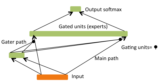
Figure 1: Conditional computation architecture: gater path on the left produces sparse outputs $h_{i}$ which are multiplied elementwise by the expert outputs, hidden units $H_{i}$.

5 Conditional Computation Experiments

We consider the potential application of stochastic neurons in the context of conditional computation, where the stochastic neurons are used to select which parts of some computational graph should be actually computed, given the current input. The particular architecture we experimented with is a neural network with a large hidden layer whose units $H_{i}$ will be selectively turned off by gating units $h_{i}$, i.e., the output of the i-th hidden unit is $H_{i}h_{i}$, as illustrated in Figure 1. For this to make sense in the context of conditional computation, we want $h_{i}$ to be non-zero only a small fraction $\alpha$ of the time (10% in the experiments) while the amount of computation required to compute $h_{i}$ should be much less than the amount of computation required to compute $H_{i}$. In this way, we can first compute $h_{i}$ and only compute $H_{i}$ if $h_{i}\neq 0$, thereby saving much computation. To achieve this, we connect the previous layer to $h_{i}$ through a bottleneck layer. Hence if the previous layer (or the input) has size $N$ and the main path layer also has size $N$ (i.e., $i\in\{1,\ldots N\}$), and the gater’s bottleneck layer has size $M\ll N$, then computing the gater output is $O(MN)$, which can reduce the main path computations from $O(N^{2})$ to $O(\alpha N^{2})$.

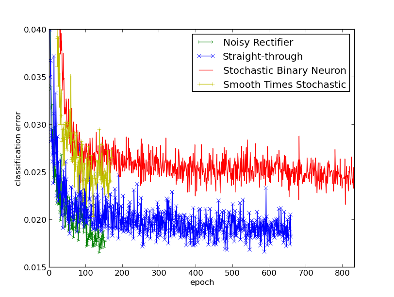
	train	valid	test
Noisy Rectifier	6.7e-4	1.52	1.87
Straight-through	3.3e-3	1.42	1.39
Smooth Times Stoch.	4.4e-3	1.86	1.96
Stoch. Binary Neuron	9.9e-3	1.78	1.89
Baseline Rectifier	6.3e-5	1.66	1.60
Baseline Sigmoid+Noise	1.8e-3	1.88	1.87
Baseline Sigmoid	3.2e-3	1.97	1.92

Figure 2: Left: Learning curves for the various stochastic approaches applied to the MNIST dataset. The y-axis indicates classification error on the validation set. Right: Comparison of training criteria and valid/test classification error (%) for stochastic (top) and baseline (bottom) gaters.

Experiments are performed with a gater of 400 hidden units and 2000 output units. The main path also has 2000 hidden units. A sparsity constraint is imposed on the 2000 gater output units such that each is non-zero 10% of the time, on average. The validation and test errors of the stochastic models are obtained after optimizing a threshold in their deterministic counterpart used during testing. See the appendix in supplementary material for more details on the experiments.

For this experiment, we compare with 3 baselines. The Baseline Rectifier is just like the noisy rectifier, but with 0 noise, and is also constrained to have a sparsity of 10%. The Baseline Sigmoid is like the STS and ST models in that the gater uses sigmoids for its output and tanh for its hidden units, but has no sparsity constraint and only 200 output units for the gater and main part. The baseline has the same hypothetical resource constraint in terms of computational efficiency (run-time), but has less total parameters (memory). The Baseline Sigmoid with Noise is the same, but with Gaussian noise added during training.

6 Conclusion

In this paper, we have motivated estimators of the gradient through highly non-linear non-differentiable functions (such as those corresponding to an indicator function), especially in networks involving noise sources, such as neural networks with stochastic neurons. They can be useful as biologically motivated models and they might be useful for engineering (computational efficiency) reasons when trying to reduce computation via conditional computation or to reduce interactions between parameters via sparse updates (Bengio, 2013). We have proven interesting properties of three classes of stochastic neurons, the noisy rectifier, the STS unit, and the binary stochastic neuron, in particular showing the existence of an unbiased estimator of the gradient for the latter. Unlike the SPSA (Spall, 1992) estimator, our estimator is unbiased even though the perturbations are not small (0 or 1), and it multiplies by the perturbation rather than dividing by it.

Experiments show that all the tested methods actually allow training to proceed. It is interesting to note that the gater with noisy rectifiers yielded better results than the one with the non-noisy baseline rectifiers. Similarly, the sigmoid baseline with noise performed better than without, even on the training objective: all these results suggest that injecting noise can be useful not just as a regularizer but also to help explore good parameters and fit the training objective. These results are particularly surprising for the stochastic binary neuron, which does not use any backprop for getting a signal into the gater, and opens the door to applications where no backprop signal is available. In terms of conditional computation, we see that the expected saving is achieved, without an important loss in performance. Another surprise is the good performance of the straight-through units, which provided the best validation and test error, and are very simple to implement.

Acknowledgments

The authors would like to acknowledge the useful comments from Guillaume Alain and funding from NSERC, Ubisoft, CIFAR (YB is a CIFAR Fellow), and the Canada Research Chairs.

Appendix A Details of the Experiments

We frame our experiments using a conditional computation architecture. We limit ourselves to a simple architecture with 4 affine transforms. The output layer consists of an affine transform followed by softmax over the 10 MNIST classes. The input is sent to a gating subnetwork and to an experts subnetwork, as in Figure 1. There is one gating unit per expert unit, and the expert units are hidden units on the main path. Each gating unit has a possibly stochastic non-linearity (different under different algorithms evaluated here) applied on top of an affine transformation of the gater path hidden layer (400 tanh units that follow another affine transformation applied on the input). The gating non-linearity are either Noisy Rectifiers, Smooth Times Stochastic (STS), Stochastic Binary Neurons (SBN), Straight-through (ST) or (non-noisy) Rectifiers over 2000 units.

The expert hidden units are obtained through an affine transform without any non-linearity, which makes this part a simple linear transform of the inputs into 2000 expert hidden units. Together, the gater and expert form a conditional layer. These could be stacked to create deeper architectures, but this was not attempted here. In our case, we use but one conditional layer that takes its input from the vectorized 28x28 MNIST images. The output of the conditional layer is the element-wise multiplication of the (non-linear) output of the gater with the (linear) output of the expert. The idea of using a linear transformation for the expert is derived from an analogy over rectifiers which can be thought of as the product of a non-linear gater ($\mathbf{1}_{h_{i}>0}$) and a linear expert ($h_{i}$).

A.1 Sparsity Constraint

Computational efficiency is gained by imposing a sparsity constraint on the output of the gater. All experiments aim for an average sparsity of 10%, such that for 2000 expert hidden units we will only require computing approximately 200 of them in average. Theoretically, efficiency can be gained by only propagating the input activations to the selected expert units, and only using these to compute the network output. For imposing the sparsity constraint we use a KL-divergence criterion for sigmoids and an L1-norm criterion for rectifiers, where the amount of penalty is adapted to achieve the target level of average sparsity.

A sparsity target of $s=0.1$ over units $i=1...2000$, each such unit having a mean activation of $p_{i}$ within a mini-batch of 32 propagations, yields the following KL-divergence training criterion:

$${\rm KL}(s||p)=-\lambda\sum_{i}{\left(s\log{p_{i}}+(1-s)\log{1-p_{i}}\right)}$$ (14)

where $\lambda$ is a hyper-parameter that can be optimized through cross-validation. In the case of rectifiers, we use an L1-norm training criteria:

$${\rm L1}(p)=\lambda\sum{|p_{i}|}$$ (15)

In order to keep the effective sparsity $s_{e}$ (the average proportion of non-zero gater activations in a batch) of the rectifier near the target sparsity of $s=0.1$, $\lambda$ is increased when $s_{e}>s+0.01$, and reduced when $s_{e}<s-0.01$. This simple approach was found to be effective at maintaining the desired sparsity.

A.2 Beta Noise

There is a tendency for the KL-divergence criterion to keep the sigmoids around the target sparsity of $s=0.1$. This is not the kind of behavior desired from a gater, it indicates indecisiveness on the part of the gating units. What we would hope to see is each unit maintain a mean activation of $0.1$ by producing sigmoidal values over 0.5 approximately 10% of the time. This would allow us to round sigmoid values to zero or one at test time.

In order to encourage this behavior, we introduce noise at the input of the sigmoid, as in the semantic hashing algorithm (Salakhutdinov and Hinton, 2009). However, since we impose a sparsity constraint of 0.1, we have found better results with noise sampled from a Beta distribution (which is skewed) instead of a Gaussian distribution. To do this we limit ourselves to hyper-optimizing the $\beta$ parameter of the distribution, and make the $\alpha$ parameter a function of this $\beta$ such that the mode of the distribution is equal to our sparsity target of 0.1. Finally, we scale the samples from the distribution such that the sigmoid of the mode is equal to 0.1. We have observed that in the case of the STS, introducing noise with a $\beta$ of approximately 40.1 works bests. We considered values of 1.1, 2.6, 5.1, 10.1, 20.1, 40.1, 80.1 and 160.1. We also considered Gaussian noise and combinations thereof. We did not try to introduce noise into the SBN or ST sigmoids since they were observed to have good behavior in this regard.

A.3 Test-time Thresholds

Although injecting noise is useful during training, we found that better results could be obtained by using a deterministic computation at test time, thus reducing variance, in a spirit of dropout (Hinton et al., 2012). Because of the sparsity constraint with a target of 0.1, simply thresholding sigmoids at 0.5 does not yield the right proportion of 0’s. Instead, we optimized a threshold to achieve the target proportion of 1’s (10%) when running in deterministic mode.

A.4 Hyperparameters

The noisy rectifier was found to work best with a standard deviation of 1.0 for the gaussian noise. The stochastic half of the Smooth Times Stochastic is helped by the addition of noise sampled from a beta distribution, as long as the mean of this distribution replaces it at test time. The Stochastic Binary Neuron required a learning rate 100 times smaller for the gater (0.001) than for the main part (0.1). The Straight-Through approach worked best without multiplying the estimated gradient by the derivative of the sigmoid, i.e. estimating $\frac{\partial L}{\partial a_{i}}$ by $\frac{\partial L}{\partial h_{i}}$ where $h_{i}=\mathbf{1}_{z_{i}>{\rm sigm}(a_{i})}$ instead of $\frac{\partial L}{\partial h_{i}}(1-{\rm sigm}(a_{i})){\rm sigm}(a_{i})$. Unless indicated otherwise, we used a learning rate of 0.1 throughout the architecture.

We use momentum for STS, have found that it has a negative effect for SBN, and has little to no effect on the ST and Noisy Rectifier units. In all cases we explored using hard constraints on the maximum norms of incoming weights to the neurons. We found that imposing a maximum norm of 2 works best in most cases.

References

- Bengio (2013) Bengio, Y. (2013). Deep learning of representations: Looking forward. Technical Report arXiv:1305.0445, Universite de Montreal.
- Bengio et al. (2013) Bengio, Y., Courville, A., and Vincent, P. (2013). Unsupervised feature learning and deep learning: A review and new perspectives. IEEE Trans. Pattern Analysis and Machine Intelligence (PAMI).
- Dayan (1990) Dayan, P. (1990). Reinforcement comparison. In Connectionist Models: Proceedings of the 1990 Connectionist Summer School, San Mateo, CA.
- El Hihi and Bengio (1996) El Hihi, S. and Bengio, Y. (1996). Hierarchical recurrent neural networks for long-term dependencies. In NIPS 8. MIT Press.
- Fiete and Seung (2006) Fiete, I. R. and Seung, H. S. (2006). Gradient learning in spiking neural networks by dynamic perturbations of conductances. Physical Review Letters, 97(4).
- Glorot et al. (2011) Glorot, X., Bordes, A., and Bengio, Y. (2011). Deep sparse rectifier neural networks. In AISTATS.
- Goodfellow et al. (2013) Goodfellow, I. J., Warde-Farley, D., Mirza, M., Courville, A., and Bengio, Y. (2013). Maxout networks. In ICML’2013.
- Hinton (2012) Hinton, G. (2012). Neural networks for machine learning. Coursera, video lectures.
- Hinton et al. (1984) Hinton, G. E., Sejnowski, T. J., and Ackley, D. H. (1984). Boltzmann machines: Constraint satisfaction networks that learn. Technical Report TR-CMU-CS-84-119, Carnegie-Mellon University, Dept. of Computer Science.
- Hinton et al. (2012) Hinton, G. E., Srivastava, N., Krizhevsky, A., Sutskever, I., and Salakhutdinov, R. (2012). Improving neural networks by preventing co-adaptation of feature detectors. Technical report, arXiv:1207.0580.
- Krizhevsky et al. (2012a) Krizhevsky, A., Sutskever, I., and Hinton, G. (2012a). ImageNet classification with deep convolutional neural networks. In NIPS’2012.
- Krizhevsky et al. (2012b) Krizhevsky, A., Sutskever, I., and Hinton, G. (2012b). ImageNet classification with deep convolutional neural networks. In Advances in Neural Information Processing Systems 25 (NIPS’2012).
- Nair and Hinton (2010) Nair, V. and Hinton, G. E. (2010). Rectified linear units improve restricted Boltzmann machines. In ICML’10.
- Rumelhart et al. (1986) Rumelhart, D. E., Hinton, G. E., and Williams, R. J. (1986). Learning representations by back-propagating errors. Nature, 323, 533–536.
- Salakhutdinov and Hinton (2009) Salakhutdinov, R. and Hinton, G. (2009). Semantic hashing. In International Journal of Approximate Reasoning.
- Spall (1992) Spall, J. C. (1992). Multivariate stochastic approximation using a simultaneous perturbation gradient approximation. IEEE Transactions on Automatic Control, 37, 332–341.
- Vincent et al. (2008) Vincent, P., Larochelle, H., Bengio, Y., and Manzagol, P.-A. (2008). Extracting and composing robust features with denoising autoencoders. In ICML 2008.
- Weaver and Tao (2001) Weaver, L. and Tao, N. (2001). The optimal reward baseline for gradient-based reinforcement learning. In Proc. UAI’2001, pages 538–545.
- Williams (1992) Williams, R. J. (1992). Simple statistical gradient-following algorithms connectionist reinforcement learning. Machine Learning, 8, 229–256.