Inadmissibility of the best equivariant predictive density in the unknown variance case

1 Introduction

The most natural way to estimate an unobserved quantity $\mu$ is to use observed averages. However, Stein (1956) demonstrated the inadmissibility of such estimators when $\mu\in\mathbb{R}^{d}$ with $d\geq 3$; that is, he showed that there exist better estimators. The notion of better estimator means here that it has a lower quadratic risk $R_{Q}(\mu,\hat{\mu})=\operatorname{\textit{E}}_{\mu}(\|\hat{\mu}-\mu\|^{2})$, where $\hat{}\mu$ is an estimator of $\mu$ and the expectation is taken with respect to random quantities used in the construction of $\hat{}\mu$. This phenomenon, the Stein effect, was first brought to light in the context of parameter estimation. For such a problem, many classes of estimators dominating the average have been proposed.

In parallel, a similar phenomenon has been observed for predictive density estimation. For instance, let us observe $n$ independent $d$-dimensional vectors $x_{1},\dots,x_{n}$, each supposedly normally distributed, $x_{i}\sim N_{d}(\mu,\sigma^{2}\,{I}_{d})$ $(i=1,\dots,n)$, where the common mean $\mu$ is unknown, and the covariance matrix $\sigma^{2}\,{I}_{d}$ is assumed known. The aim is to estimate the density of a future vector $y$, which is also assumed to be normal with same mean and variance, $y\sim N_{d}(\mu,\sigma^{2}\,{I}_{d})$. In this context, the mean $\bar{x}=n^{-1}\sum_{i=1}^{n}x_{i}$ is a sufficient statistic used for the estimation of the predictive density by a function $\hat{p}(y\mid\bar{x})$. The quality of such an estimator is often measured by the Kullback–Leibler risk

$$R_{KL}(\mu,\hat{p})=\int\phi(\bar{x};\mu,\sigma^{2}/n)\!\int\!\phi(y;\mu,\sigma^{2})\log\frac{\phi(y;\mu,\sigma^{2})}{\hat{p}(y\mid\bar{x})}dyd\bar{x},$$

where $\phi(\cdot;\theta,\tau)$ is the multivariate Gaussian density with mean vector $\theta$ and covariance matrix $\tau{I}_{d}$. The most natural way to estimate $\phi(y;\mu,\sigma^{2})$ is to just plug in an estimator of $\mu$, yielding $\hat{p}(y\mid\bar{x})=\phi\{y;\mu=\hat{}\mu(\bar{x}),\sigma^{2}\}$. However, Aitchison (1975) proved that plug-in densities are uniformly dominated under the Kullback–Leibler risk by the best equivariant predictive density, which is a Bayesian predictive density taken with respect to the uniform prior $\pi_{U}(\mu)=1$, and is given by $\hat{p}_{U}(y\mid\bar{x})=\phi\{y;\bar{x},(n+1)\sigma^{2}/n\}$. George et al. (2006) have shown that predictive density estimation and parameter estimation are closely related. They argue that the best equivariant predictive density $\hat{p}_{U}(y\mid\bar{x})$ shares many properties with the maximum likelihood estimator: minimaxity, invariance, constant risk, and inadmissibility for dimension greater or equal to three. Hence, it should be taken as the reference estimator. Komaki (2001) showed that, when $d\geq 3$, it is dominated by the Bayesian predictive density with respect to the harmonic prior $\pi_{H}(\mu)=\|\mu\|^{-(d-2)}$, also known as the shrinkage prior.

A more interesting and practical setting is when the variance $\sigma^{2}$ is unknown. In such a case, the sufficient statistic is $(\bar{x},s)$, where $s=\sum_{i=1}^{n}\|x_{i}-\bar{x}\|^{2}$ estimates the variance up to a factor. The Kullback–Leibler risk becomes

$$R_{KL}\{(\mu,\sigma^{2}),\hat{p}\}=\iint\!\phi(\bar{x};\mu,\sigma^{2}\!/n)\frac{\gamma\{s/\sigma^{2};(n-1)d\}}{\sigma^{2}}\!\int\!\phi(y;\mu,\sigma^{2})\log\frac{\phi(y;\mu,\sigma^{2})}{\hat{p}(y\mid\bar{x},s)}dyd\bar{x}ds,$$

where $\gamma(\cdot;\upsilon)$ is the chi-square density with degrees of freedom $\upsilon$. The best equivariant predictive density is now taken with respect to the right invariant prior $\pi_{R}(\mu,\sigma)=1/\sigma$ and is the Student $t$-distribution (Liang & Barron, 2004)

$$\hat{p}_{R}(y\mid\bar{x},s)=c_{R}\left(\frac{1}{\pi s}\,\frac{n}{n+1}\right)^{d/2}\left(1+\frac{1}{s}\frac{n}{n+1}\|y-\bar{x}\|^{2}\right)^{-nd/2},$$

where $c_{R}=\Gamma(nd/2)/\Gamma\{(n-1)d/2\}$ and $\Gamma(\cdot)$ denotes the Gamma function. So far, there are very few results on admissibility of $\hat{p}_{R}$. Three papers propose extensions to the harmonic prior $\pi_{H}$, and have influenced the present paper. The first is due to Kato (2009), who showed that, for $d\geq 3$ and under the Kullback–Leibler risk, the best equivariant density $\hat{p}_{R}$ is dominated by the Bayesian predictive density with respect to the prior

$$\pi_{K}(\mu,\eta)=\int_{0}^{1}\phi\left\{\mu;0,\eta^{-1}\lambda^{-1}(1-\lambda)\right\}\pi(\eta,\lambda)d\lambda,\quad\pi(\eta,\lambda)=\eta^{-2}\lambda^{-2}1_{(0,1)}(\lambda),$$ (1)

where $\eta=1/\sigma^{2}$ and $1_{A}(x)=1$ if $x\in A$ and $0$ otherwise. Komaki (2006, 2007) considered a prior based on the Green’s function of the manifold of the unknown variance model, which is a hyperbolic plane. In an asymptotic framework, he showed the inadmissibility of the best equivariant predictive density under the Kullback–Leibler risk even when $d<3$. Finally, Maruyama & Strawderman (2012) uses an extension of the prior $\pi_{K}$ given by equation (1) with

$$\pi(\eta,\lambda)=\eta^{a}\lambda^{a}(1-\lambda)^{b}\,1_{(0,1)}(\lambda),$$ (2)

where $a$ and $b$ are constants. This prior leads to an estimator of the density dominating the best equivariant density also in the low dimensional case, where $d=1$ or 2. Unlike Komaki (2007)’s result, the latter one was obtained in a nonasymptotic framework, and under the risk

$$R_{1}\{(\mu,\sigma^{2}),\hat{p}\}=\iint\!\phi(\bar{x};\mu,\sigma^{2}\!/n)\frac{\gamma\{s/\sigma^{2};(n-1)d\}}{\sigma^{2}}\!\int\!\hat{p}(y\mid\bar{x},s)\log\frac{\hat{p}(y\mid\bar{x},s)}{\phi(y;\mu,\sigma^{2})}dyd\bar{x}ds,$$

which is denoted by $R_{1}$ because it corresponds to Csiszár’s $\alpha$-divergence with $\alpha=1$.

In the present work, we consider the Kullback–Leibler risk, which is another special case of Csiszár’s $\alpha$-divergence with $\alpha=-1.$ In the context of unknown variance we show that the inadmissibility of the best equivariant predictive density $\hat{p}_{R}$ for any $d$, even $d=1$ or 2, remains true under the Kullback–Leibler risk, hence extending Kato (2009)’s result. Furthermore, we partially solve Problem 2-2 stated by Maruyama & Strawderman (2012), namely, “Under $d=1,2$ and the $R_{\alpha}$-risk with $-1\leq\alpha<1$, does the best invariant predictive density keep inadmissibility? If so, which Bayesian predictive densities improve it?”. We consider an extension of the harmonic prior different from that of Komaki (2007), but the major difference lies in the fact that we have nonasymptotic results. Such results are derived under the Gaussian assumption, whereas Komaki (2007) considered a more general distribution. Finally, we establish a preliminary basis for comparing the estimation and prediction problems for the unknown variance setting, in a similar fashion to George et al. (2006). Such a comparison is however much more difficult to prove formally than for the known variance case, thus remaining an open problem.

2 The Bayesian predictive density under unknown variance

We are interested in estimating the predictive density of

$$y\sim N_{d}(\mu,\sigma^{2}\,{I}_{d}),$$ (3)

based on the observations $x_{1},\dots,x_{n}$, where $x_{i}\sim N_{d}(\mu,\sigma^{2}\,{I}_{d})$.

In this section, we aim at extending the result of George et al. (2006) expressing a Bayesian predictive density with respect to a prior $\pi$ as a function of the best equivariant density, i.e.,

$$\hat{p}_{\pi}(y\mid\bar{x}_{n})=\frac{m_{\pi}\{\bar{x}_{n+1};(n+1)^{-1}\eta^{-1}\}}{m_{\pi}(\bar{x}_{n};n^{-1}\eta^{-1})}\;\hat{p}_{U}(y\mid\bar{x}_{n}),\quad m_{\pi}(z;\sigma^{2})=\int\phi\left(z;\mu,\sigma^{2}\right)\pi(\mu)d\mu,$$

where $\bar{x}_{n}=\bar{x}$, $\bar{x}_{n+1}=(n\bar{x}_{n}+y)/(n+1)$ and $\eta=1/\sigma^{2}$. Theorem 2.1 gives a similar expression for the unknown variance case, relying on both the sufficient statistic $(\bar{x},s)$ and the statistic $(\bar{x}_{n+1},s_{n+1})$, with

$$\bar{x}_{n+1}\sim N_{d}\left\{\mu,(n+1)^{-1}\eta^{-1}{I}_{d}\right\},\quad s_{n+1}=s_{n}+n\|y-\bar{x}_{n}\|^{2}/(n+1)\sim\eta^{-1}\chi_{nd}^{2},$$

where $s_{n}=s.$ The marginal density $m_{\pi}(z,v;l)$ is defined for $z\sim N_{d}\{\mu,(l\eta)^{-1}{I}_{d}\}$ and $v\sim\eta^{-1}\chi_{(l-1)d}^{2}$ by

$$m_{\pi}(z,v;l)=\iint\phi\left(z;\mu,l^{-1}\eta^{-1}\right)\eta\,\gamma\left\{\eta v;(l-1)d/2\right\}\pi(\mu,\eta)d\mu\,d\eta.$$

Theorem 2.1.

For any prior $\pi(\mu,\eta)$, the Bayesian predictive density can be expressed as

$$\hat{p}_{\pi}(y\mid\bar{x}_{n},s_{n})=\frac{\rho_{\pi}(\bar{x}_{n+1},s_{n+1};n+1)}{\rho_{\pi}(\bar{x}_{n},s_{n};n)}\,\hat{p}_{R}(y\mid\bar{x}_{n},s_{n}),$$

where $\hat{p}_{R}(y\mid\bar{x}_{n},s_{n})$ is the best equivariant predictive density and $\rho_{\pi}=v\,m_{\pi}(z,v;l)$. Furthermore, the difference between the Kullback–Leibler risks of $\hat{p}_{\pi}$ and $\hat{p}_{R}$ is

$$R_{KL}\{(\mu,\eta),\hat{p}_{R}\}-R_{KL}\{(\mu,\eta),\hat{p}_{\pi}\}=\operatorname{\textit{E}}_{(\mu,\eta)}\!\left\{\log\frac{\rho_{\pi}(\bar{x}_{n+1},s_{n+1};n+1)}{\rho_{\pi}(\bar{x}_{n},s_{n};n)}\right\}\!,$$

where $\operatorname{\textit{E}}_{(\mu,\eta)}$ denotes the expectation with respect to $(y,\bar{x},s)$, provided the expectations exist.

Unfortunately, we have not been able to link such an expression directly to the estimation problem, as was done by George et al. (2006), but we believe that the link exists and in Section 5 we give some leads to uncover it.

3 Inadmissibility of the best equivariant density

3.1 Choice of prior

The easiest way to show the inadmissibility of an estimator is to exhibit a dominating estimator. Below, we prove the inadmissibility of the best equivariant density by showing that it is dominated by the Bayesian predictive density with respect to the prior

$$\pi_{\rm GM}(\mu,\eta)=\int_{0}^{1}\phi\left\{\mu;0,\eta^{-1}\lambda^{-1}(1-\lambda)\right\}\pi(\eta,\lambda)d\lambda,\quad\pi(\eta,\lambda)=\eta^{a}\lambda^{a}\widetilde{\pi}(\lambda)\,1_{(0,1)}(\lambda),$$ (4)

where the subscript ${\rm GM}$ stands for Gaussian mixture. The function $\widetilde{\pi}(\lambda)$ will be specified later. The priors studied by Kato (2009) and Maruyama & Strawderman (2012) are special cases of this class of priors with $a=-2$ and $\widetilde{\pi}(\lambda)=1$ and $\widetilde{\pi}(\lambda)=(1-\lambda)^{b}$.

We separate two cases, the low-dimensional case where $d\leq 4$, and the higher-dimensional case where $d\geq 3$.

3.2 Domination for the low dimensional case

Setting $\nu=d/2+a+1>0$, we consider the following special case for the prior in (4),

$$\widetilde{\pi}(\lambda)=(1-\lambda)^{(n-1)d/2-1}\left\{1-(n-1)\lambda/n\right\}^{-(n-2)d/2-\nu},\quad\lambda\in(0,1).$$ (5)

Theorem 3.1.

If $d\leq 4$ and $n=2$, the best equivariant density $\hat{p}_{R}$ is inadmissible under the Kullback–Leibler risk in the unknown variance setting. In particular, it is dominated by the Bayesian predictive density with respect to the prior $\pi_{\rm GM}$ where the function $\widetilde{\pi}$ is specified by equation (5) with $0<\nu\leq\nu_{*}$, $\nu_{*}$ being constant.

Proof.

The difference in Kullback–Leibler risks between a Bayesian predictive density $\hat{p}_{\pi}$ and the best equivariant one is

$$R_{KL}\{(\mu,\eta),\hat{p}_{R}\}-R_{KL}\{(\mu,\eta),\hat{p}_{\pi}\}=\operatorname{\textit{E}}_{(\mu,\eta)}\!\left\{\log\frac{\hat{p}_{\pi}(y\mid\bar{x}_{n},s_{n})}{\hat{p}_{R}(y\mid\bar{x}_{n},s_{n})}\,\right\}\!.$$

From Lemma A1, and for the prior $\pi_{\rm GM}$, where the function $\widetilde{\pi}$ is specified by (5), this difference in risks is

$$R_{KL}\{(\mu,\eta),\hat{p}_{R}\}-R_{KL}\{(\mu,\eta),\hat{p}_{\rm GM}\} =\operatorname{\textit{E}}_{(\mu,\eta)}\!\bigg{[}\log\bigg{\{}c_{B}\left(\frac{n+1}{n}\right)^{\nu}\left(\frac{s_{n+1}}{s_{n}}\right)^{-\nu}\frac{J_{n+1}}{J_{n}}\bigg{\}}\bigg{]}$$

$$=\operatorname{\textit{E}}_{(\mu,\eta)}\!\left[\log\left\{c_{B}\frac{J_{n+1}}{J_{n}}\left(\frac{1-u_{n}}{1-u_{n+1}}\right)^{\nu}\right\}\right]$$

$$\qquad+\nu\operatorname{\textit{E}}_{(\mu,\eta)}\!\bigg{[}\log\bigg{\{}\frac{n+1}{n}\left(\frac{s_{n+1}}{s_{n}}\right)^{-1}\frac{1-u_{n+1}}{1-u_{n}}\bigg{\}}\bigg{]}\!,$$

where $c_{B}=B\{\nu,(n-1)d/2\}/B(\nu,nd/2)$, $u_{l}=l\|\bar{x}_{l}\|^{2}/(l\|\bar{x}_{l}\|^{2}+s_{l})$ and $J_{l}$ is given in Equation (8), for $l\in\{n,n+1\}$. By Lemmas A2 and A3, the risk difference is bounded by

$$R_{KL}\{(\mu,\eta),\hat{p}_{R}\}-R_{KL}\{(\mu,\eta),\hat{p}_{\rm GM}\}\geq\nu\operatorname{\textit{E}}(1-u_{n+1})\left\{g(n,d,\nu)-h(n,d)\right\}.$$

Since $\nu>0$ and $1-u_{n+1}\geq 0$, the sign of the lower bound is determined by the sign of $\{g(n,d,\nu)-h(n,d)\}$. Applying Lemma A4 completes the proof. ∎

Numerical computations give the following approximate values of the constant $\nu_{*}$: $\nu_{*}\approx 0.25$ for $d=1$, $\nu_{*}\approx 0.33$ for $d=2$, $\nu_{*}\approx 0.18$ for $d=3$, and $\nu_{*}\approx 0.05$ for $d=4$.

Theorem 3.1 solves Problem 2.2 stated by Maruyama & Strawderman (2012) for the Kullback–Leibler risk. A similar result has been obtained by Komaki (2007) asymptotically with the number of observations, that is, when $n\rightarrow\infty$, while here we give it in a nonasymptotic framework for $n=2$, this restriction coming from Lemma A4. From both results we conjecture that the inadmissibility also stands for $2<n<\infty$.

3.3 Domination in higher dimension

The domination of the Bayesian predictive density $\hat{p}_{\rm GM}$ over the best equivariant one $\hat{p}_{R}$ does not only occur when $d\leq 4$. Indeed, the following result shows that the domination is still true in higher dimension $d$, and larger number $n$ of observations, when this time the function $\widetilde{\pi}$ is subject to the following condition, for $0<\nu\leq d/2-1$,

$$\left\{1-n\lambda/(n+1)\right\}^{d/2-\nu-1}\leq\widetilde{\pi}(\lambda)\leq\left\{1-(n-1)\lambda/n\right\}^{d/2-\nu-1}.$$ (6)

In this setting, the inadmissibility of the best equivariant predictive density was proved by Kato (2009). However, only one improving Bayesian predictive density had been provided, whereas we give a class of such dominating densities, including that studied by Kato (2009).

Theorem 3.2.

If $d\geq 3$ and $n\geq 2$, the best equivariant density $\hat{p}_{R}$ is inadmissible under the Kullback–Leibler risk in the unknown variance setting. It is dominated by the Bayesian predictive density with respect to the prior $\pi_{\rm GM}$ where $\widetilde{\pi}$ is specified by (6).

Proof.

Direct calculations show that the lower bound in (6) results in the inequalities where

$$I_{l}=\int_{0}^{1}t^{\nu-1}\left(1+w_{l}t\right)^{-(l-1)d/2-\nu}dt=w_{l}^{-\nu}\int_{0}^{u_{l}}z^{\nu-1}(1-z)^{(l-1)d/2-1}dz,$$ (7)

the latter equality deriving from the change of variables $z=w_{l}t/(1+w_{l}t)$, with $dt=w_{l}^{-1}(1-z)^{-2}dz$, where $w_{l}=l\|\bar{x}_{l}\|^{2}/s_{l}$ and $u_{l}=w_{l}/(1+w_{l})$. Gathering those elements, the risk difference can thus be bounded as follows

$$\begin{split}R_{KL}\{(\mu,\eta),\hat{p}_{R}\}-R_{KL}\{(\mu,\eta),\hat{p}_{\rm GM}\}&\geq\nu\operatorname{\textit{E}}_{(\mu,\eta)}\!\left(\log\left\|\bar{x}_{n}\right\|^{2}-\log\|\bar{x}_{n+1}\|^{2}\right)+r_{n+1}-r_{n},\end{split}$$

where $r_{l}=\operatorname{\textit{E}}\{\log F_{l}(u_{l})\}$, $l\in\{n,n+1\}$, with

$$F_{l}(u)=\frac{1}{B\{\nu,(l-1)d/2\}}\int_{0}^{u}t^{\nu-1}(1-t)^{(l-1)d/2-1}dt,\quad u\in(0,1),$$

and the expectation being taken with respect to $u_{l}$. This latter inequality is an equality for the prior $\pi_{K}$ considered by Kato (2009). Based on Komaki (2001), we have that

$$\operatorname{\textit{E}}_{(\mu,\eta)}\!\!\left(\log\left\|\bar{x}_{n}\right\|^{2}-\log\|\bar{x}_{n+1}\|^{2}\right)\geq 0.$$

Finally, after a few calculations, we obtain that

$$r_{n+1}-r_{n}\geq\operatorname{\textit{E}}\!\left[\log F_{n+1}\!\left\{\frac{\chi^{2}_{d}(n\xi)}{\chi^{2}_{d}(n\xi)+\chi^{2}_{nd}}\right\}\right]-\operatorname{\textit{E}}\!\left[\log F_{n}\!\left\{\frac{\chi^{2}_{d}(n\xi)}{\chi^{2}_{d}(n\xi)+\chi^{2}_{(n-1)d}}\right\}\right]\!.$$

From Kato (2009), this latter lower bound is positive, thus completing the proof. ∎

The case $d=n=2$ makes the link between the two settings. Indeed, in such a case, the function $\widetilde{\pi}$ defined by equation (5) and the upper bound given in equation (6) both equal $(1-\lambda/2)^{-\nu}$.

Finally, the prior considered by Maruyama & Strawderman (2012) and given in (2) also belongs to the same class of priors as those specified in the current section, and leads to improvement under the $R_{1}$-risk. This class of priors thus seems to be of special interest and may even include a universal prior leading to improvement for any dimension $d$, number $n$ of observations, and any loss. However, we have not yet been able to exhibit such a prior.

4 Numerical experiment

In order to check the results of Theorem 3.1, we considered the example given by Kato (2009). The experiment is driven for values of the noncentral parameter $\xi=\eta\|\mu\|^{2}$ taken in $[0,1\!~{}000]$, and values of the shape parameter $\nu$ taken in $\{0.05,0.25,0.50,\dots,1.75,2\}$. We estimate the difference in risks over $r=5\!~{}000$ replicates of the different random variables involved and average the results over 10 trials of such an experiment.

Figure 1 shows the behaviour of the estimated difference in risks as a function of $\xi$ and $\nu$ for each $d\in\{1,2,3\}$ when $n=2$. In this figure, the difference in risks is indeed positive for any $\xi$ and within the range defined by Theorem 3.1 for $\nu$, thus confirming our theoretical results. What is perhaps more surprising is that the difference in risks is still positive for larger values of $\nu$. This is especially noticeable in the case $d=3$, where the largest improvement seems to be obtained for $\nu\in[1,2]$, whereas in theory we could only prove domination when $\nu\leq 0.18$.

$d=1$ $d=2$ $d=3$

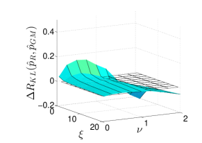
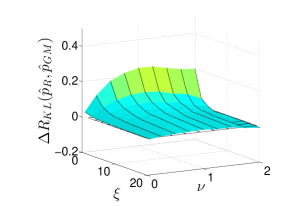
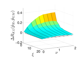
Figure 1: Difference in Kullback–Leibler risks as a function of the noncentrality parameter $\xi=\eta\|\mu\|^{2}$ and of the shape parameter $\nu$, for $d\leq 3$ and $n=2$. The black grid shows the plane $z=0$.

5 Discussion

Although we have not been able to prove it so far, it is our conviction that there exists a link between the prediction problem and the estimation problem in the unknown variance case, just as has been shown in the known variance case (George et al., 2006). In order to make this clear, recall that Brown (1979) argues that some decision-theoretic properties do not seem to depend on the choice of the loss function. This claim concerns the estimation problem, but the work of Maruyama & Strawderman (2012), of Komaki (2007) and the present work, showing inadmissibility of the best equivariant predictive density for any dimension under two different losses, seem to verify it for the prediction problem as well. Such a relationship is particularly appealing since it was proved by Maruyama & Strawderman (2012) that there exists a direct link between prediction under $R_{1}$-risk and simultaneous estimation of the mean $\mu$ and the variance $\sigma^{2}$. Indeed, the authors show that, for $\pi$ given in equation (2),

$$R_{1}\{(\mu,\sigma^{2}),\hat{p}_{\pi}\}=c_{IQ}\operatorname{\textit{E}}_{(\mu,\sigma^{2})}\!\left(\|\hat{\mu}_{\pi}-\mu\|^{2}/\sigma^{2}\right)+c_{S}\operatorname{\textit{E}}_{(\mu,\sigma^{2})}\!\left\{\hat{\sigma}_{\pi}^{2}/\sigma^{2}-\log(\hat{\sigma}_{\pi}^{2}/\sigma^{2})-1\right\}\!,$$

where $c_{IQ}$ and $c_{S}$ are constants. In this expression, we easily recognise the invariant quadratic risk of $\hat{\mu}_{\pi}$ and Stein’s risk of $\hat{\sigma}_{\pi}^{2}$. However, this equality follows from the fact that the Bayesian predictive density under the $R_{1}$-risk reduces to a plug-in density, which is not the case here. Hence, it is not clear whether the link would still be possible under the Kullback–Leibler risk. Another reason for our conjecture is that several arguments given by George et al. (2006) are still true under the unknown variance setting: the unbiased estimator of $(\mu,\sigma^{2})$ is equal to the mean and variance of the best equivariant density, and both the unbiased estimators and the best equivariant distribution are minimax and inadmissible whatever the dimension is.

Theorem 2.1 gives an expression of the difference in risks, which can be rewritten as

$$R_{KL}\{(\mu,\sigma^{2}),\hat{p}_{R}\}-R_{KL}\{(\mu,\sigma^{2}),\hat{p}_{\pi}\}=\int_{n}^{n+1}\frac{\partial}{\partial l}\,Q(l,\mu,\sigma^{2})dl,$$

where $Q(l,\mu,\sigma^{2})=\operatorname{\textit{E}}_{(\mu,\sigma^{2})}\{\log\rho_{\pi}(z,v;l)\}$ and $\rho_{\pi}(z,v;l)=v\,m_{\pi}(z,v;l)$. Hence, a sufficient condition for the difference in risks to be positive is that $\partial Q(l,\mu,\sigma^{2})/\partial l\geq 0$ for all $(\mu,\sigma^{2})$ and for $l\in\{n,n+1\}$. This type of expression is the key element that helped George et al. (2006) explicitely express the link with the estimation problem, but its derivation is much more difficult under the unknown variance setting. It thus remains an open problem to find a similar result when the variance is unknown.

Supplementary material

The proofs of Theorems 2.1 and 3.2 and of the Lemmas given in the Appendix are provided in Supplementary Material, along with details of the simulation study.

Appendix A Lemmas used in the proof of Theorem 3.1

Lemma 1.

Under the assumptions of Model (3), the Bayesian predictive density with respect to the prior $\pi_{\rm GM}$ in (4) is

$$\hat{p}_{\rm GM}(y\mid\bar{x}_{n},s_{n})=c_{\rm GM}\left(\frac{s_{n+1}}{s_{n}}\right)^{-\nu}\frac{J_{n+1}}{J_{n}}\;\hat{p}_{R}(y\mid\bar{x}_{n},s_{n}),$$

where $c_{\rm GM}=(1+1/n)^{\nu}B\left\{\nu,(n-1)d/2\right\}/B\left(\nu,nd/2\right)$ is a constant and the term $J_{l}$, $l\in\{n,n+1\}$, is defined as

$$J_{l}=\int_{0}^{1}\frac{\lambda^{\nu-1}\{1+(l-1)\lambda\}^{d/2-\nu-1}}{\left(1+w_{l}\,\lambda\right)^{(l-1)d/2+\nu}}\,\widetilde{\pi}\!\left\{\frac{l\lambda}{1+(l-1)\lambda}\right\}d\lambda,$$ (8)

where $\nu=d/2+a+1$, $B(\cdot,\cdot)$ denotes the Beta function and $w_{l}=l\|\bar{x}_{l}\|^{2}/s_{l}$.

Lemma 2.

Let $n\geq 2$, $0<\nu<1$, and $\widetilde{\pi}$ be specified by (5). Then

$$\operatorname{\textit{E}}_{(\mu,\eta)}\!\left(\log\left[\frac{B\{\nu,(n-1)d/2\}}{B(\nu,nd/2)}\frac{J_{n+1}}{J_{n}}\frac{(1-u_{n})^{\nu}}{(1-u_{n+1})^{\nu}}\right]\right)\geq\nu\,g(n,d,\nu)\operatorname{\textit{E}}(1-u_{n+1}),$$

where $u_{l}=w_{l}/(1+w_{l})$, $l\in\{n,n+1\}$, the expectation $\operatorname{\textit{E}}(\cdot)$ is taken with respect to a noncentral Beta random variable, and the function $g$ is defined by

$$g(n,d,\nu)=\begin{cases}\displaystyle\frac{1}{\nu}\log\frac{B\{\nu,nd/2-(d-\nu)/n\}}{B(\nu,nd/2)},&d\leq n,\\ \displaystyle{\frac{1}{n\nu}\,\frac{d-\nu}{nd/2-1}}\log(1+\nu),&d\geq n+1.\end{cases}$$ (9)

Lemma 3.

Let $n\geq 2$ and $\widetilde{\pi}$ be specified by equation (5). Then,

$$\operatorname{\textit{E}}_{(\mu,\eta)}\!\left\{\log\left(\frac{n+1}{n}\,\frac{s_{n}}{s_{n+1}}\,\frac{1-u_{n+1}}{1-u_{n}}\right)\right\}\geq-h(n,d)\operatorname{\textit{E}}(1-u_{n+1}),$$

where $u_{l}=w_{l}/(1+w_{l})$, $l\in\{n,n+1\}$, the expectation $\operatorname{\textit{E}}(\cdot)$ is taken with respect to a noncentral Beta random variable, and the function $h$ is defined by

$$h(n,d)=\frac{1+(n+1)d/2}{nd/2}\left[\psi\{1+(n+1)d/2\}-\psi(1+nd/2)\right],$$ (10)

$\psi(x)=d\log\Gamma(x)/dx$ being the digamma function.

Lemma 4.

Let $n=2$ and $1\leq d\leq 4$. Then, there exists a constant $\nu_{*}$ depending only on the dimension $d$ such that, for any $0<\nu\leq\nu_{*}$,

$$g(n,d,\nu)-h(n,d)\geq 0.$$

References

• Aitchison (1975) Aitchison, J. (1975). Goodness of prediction fit. Biometrika 62, 547–554.
• Brown (1979) Brown, L.Β D. (1979). A heuristic method for determining admissibility of estimatorsβ€”with applications. Ann. Statist. 7, 960–994.
• George etΒ al. (2006) George, E.Β I., Liang, F. & Xu, X. (2006). Improved minimax predictive densities under Kullback–Leibler loss. Ann. Statist. 34, 78–91.
• Kato (2009) Kato, K. (2009). Improved prediction for a multivariate normal distribution with unknown mean and variance. Ann. Inst. Statist. Math. 61, 531–542.
• Komaki (2001) Komaki, F. (2001). A shrinkage predictive distribution for multivariate normal observables. Biometrika 88, 859–864.
• Komaki (2006) Komaki, F. (2006). Shrinkage priors for Bayesian prediction. Ann. Statist. 34, 808–819.
• Komaki (2007) Komaki, F. (2007). Bayesian prediction based on a class of shrinkage priors for location-scale models. Ann. Inst. Statist. Math. 59, 135–146.
• Liang & Barron (2004) Liang, F. & Barron, A. (2004). Exact minimax strategies for predictive density estimation, data compression, and model selection. IEEE Trans. Inform. Theory 50, 2708–2726.
• Maruyama & Strawderman (2012) Maruyama, Y. & Strawderman, W.Β E. (2012). Bayesian predictive densities for linear regression models under $\alpha$-divergence loss: Some results and open problems. In IMS Collections, Contemporary Developments in Bayesian Analysis and Statistical Decision Theory: A Festschrift for William E. Strawderman, D.Β Fourdrinier, Γ‰.Β Marchand & A.Β Rukhin, eds., vol.Β 8. Beachwood, Ohio, USA: Institute of Mathematical Statistics, pp. 42–56.
• Stein (1956) Stein, C. (1956). Inadmissibility of the usual estimator for the mean of a multivariate normal distribution. In Proceedings of the Third Berkeley Symposium on Mathematical Statistics and Probability, 1954–1955, vol. I. Berkeley and Los Angeles: University of California Press.