Maximum-likelihood estimation for diffusion processes via closed-form density expansions

Abstract

This paper proposes a widely applicable method of approximate maximum-likelihood estimation for multivariate diffusion process from discretely sampled data. A closed-form asymptotic expansion for transition density is proposed and accompanied by an algorithm containing only basic and explicit calculations for delivering any arbitrary order of the expansion. The likelihood function is thus approximated explicitly and employed in statistical estimation. The performance of our method is demonstrated by Monte Carlo simulations from implementing several examples, which represent a wide range of commonly used diffusion models. The convergence related to the expansion and the estimation method are theoretically justified using the theory of Watanabe [Ann. Probab. 15 (1987) 1–39] and Yoshida [J. Japan Statist. Soc. 22 (1992) 139–159] on analysis of the generalized random variables under some standard sufficient conditions.

t2This research was supported by the Guanghua School of Management, the Center for Statistical Sciences, and the Key Laboratory of Mathematical Economics and Quantitative Finance (Ministry of Education) at Peking University, as well as the National Natural Science Foundation of China (Project 11201009).

1 Introduction

Diffusion processes governed by stochastic differential equations (hereafter SDE) are widely used in describing the phenomenon of random fluctuations over time, and even become indispensable for analyzing high-frequency data; see, for example, Mykland and Zhang MyklandZhang2010survey . Practical application of diffusion models calls for statistical inference based on discretely monitored data. The literature has seen a wide spectrum of asymptotically efficient estimation methods, for example, those based on various contrast functions proposed in Yoshida Yoshida1992Discrete , Kessler Kessler1997 , Kessler and Sørensen KesslerSorensen1999 and the references given in Sørensen Sorensen2012survey . Taking the efficiency, feasibility and generality into account, maximum-likelihood estimation (hereafter MLE) can be a choice among others. However, for the increasingly complex real-world dynamics, likelihood functions (transition densities) are generally not known in closed-form and thus involve significant challenges in valuation. This leads to various methods of approximation and the resulting approximate MLE. The focus of this paper is to propose a widely applicable closed-form asymptotic expansion for transition density and thus to apply it in approximate MLE for multivariate diffusion process.

1.1 Background

To approximate likelihood functions, Yoshida Yoshida1992Discrete proposed to discretize continuous likelihood functions (see, e.g., Basawa and Prakasa Rao BasawaPrakasaRao1980book ); many others focused on direct approximation of likelihood functions (transition densities) for discretely monitored data, see surveys in, for example, Phillips and Yu PhillipsYu2009 , Jensen and Poulsen JENSENandPOULSEN2002 , Hurn, Jeisman and Lindsay Hurnetal2007 and the references therein. In particular, among various numerical methods, Lo Lo1988MLE proposed to employ a numerical solution of Kolmogorov equation for transition density; Pedersen Pedersen1995 , Brandt and Santa-Clara BrandtSantaClara2002 , Durham and Gallant DurhamGallant2002 , Stramer and Yan STRAMERandYAN2005 , Beskos and Roberts BeskosRoberts2005 , Beskos et al. BeskosPapaspiliopoulosRobertsFearnhead2006 , Beskos, Papaspiliopoulos and Roberts BeskosPapaspiliopoulosRoberts2009 and Elerian, Chib and Shephard Elerian2001 advocated the application of various Monte Carlo simulation methods; Yu and Phillips YuPhillips2001 developed an exact Gaussian method for models with a linear drift function; Jensen and Poulsen JENSENandPOULSEN2002 resorted to the techniques of binomial trees. Since all these numerical methods are computationally demanding, real-world implementation has necessitated the development of analytical methods for efficiently approximating transition density. An adhoc approach is to approximate the model by discretization, for example, the Euler scheme, and then use the transition density of the discretized model. Elerian Elerian1998 refined such an approximation via the second order Milstein scheme. Kessler Kessler1997 and Uchida and Yoshida UchidaYoshida2012 employed a more sophisticated normal-distribution-based approximation via higher order expansions of the mean and variance.

For approximate MLE of diffusions, Dacunha-Castelle and Florens-Zmirou DacunhaCastelleandFlorensZmirou1986 is one of the earliest attempts to apply the idea of small-time expansion of transition densities, which in principle can be made arbitrarily accurate. However, their method relies on implicit representation of moments of Brownian bridge functionals, and thus requires Monte Carlo simulation in implementation. A milestone is the ground-breaking work of Aït-Sahalia AitSahalia1999JF , AitSahalia2002Econometrica , AitSahalia2008AS , which established the theory of Hermite-polynomial-based analytical expansion for transition density of diffusion models and the corresponding approximate MLE. Along the line of Aït-Sahalia AitSahalia1999JF , AitSahalia2002Econometrica , AitSahalia2008AS , a number of substantial refinements and applications emerged in the literature of likelihood-based statistical inference (see surveys in Aït-Sahalia AitSahalia2009ARFE ); see, for example, Bakshi and Ju BakshiJu2005JB , Bakshi, Ju and Ou-Yang BakshiJu2006227 , Aït-Sahalia and Mykland AitSahaliaandPerMykland2003Annals , AitSahaliaandPerMykland2003Economstrica , Aït-Sahalia and Kimmel AitSahaliaandKimmel2007SVestimation , AitSahaliaKimmel2002TermStructureJFE , Li Li2010dampeddiffusion , Egorov, Li and Xu EgorovtimeinhomogeneousMLE , Schaumburg SCHAUMBURG2001 , Aït-Sahalia and Yu AitSahaliaandYu2006SaddleJE , Yu Yu2007 , Filipović, Mayerhofer and Schneider Filipovic2011 , Tang and Chen TangChen2009 , Xiu Xiu2011priceexpansion and Chang and Chen ChangChen2011 .

1.2 Expansion for likelihood functions and approximate MLE

Starting from the celebrated Edgeworth expansion for distribution of standardized summation of independently identically distributed random variables (see, e.g., Chapter XVI in Feller Feller1971 , Chapter 2 in Hall Hall1995 and Chapter 5 in McCullagh MCCULLAGH1987 ), asymptotic expansions have become powerful tools for statistics, econometrics and many other disciplines in science and technology. Taking dependence of random variables into account, Mykland Mykland1992AoS , Mykland1993 , Mykland1994 , Mykland1995 established the theory, calculation and various statistical applications of martingale expansion, which is further developed in Yoshida Yoshida1997martingaleexpansion , Yoshida2001martingaleexpansion .

Having an analogy with these Edgeworth-type expansions and motivated by MLE for diffusion processes, I propose a new small-time asymptotic expansion of transition density for multivariate diffusions based on the theory of Watanabe WatanabeAnalysisofWiener1987 and Yoshida Yoshida1992StatisticsSmallDiffusion , Yoshida1992MLE . However, in contrast to the traditional Edgeworth expansions, our expansion does not require the knowledge of generally implicit moments, cumulants or characteristic function of the underlying variable, and thus it is applicable to a wide range of diffusion processes. Moreover, in analogy to the verification of validity given in, for example, Bhattacharya and Ghosh BhattacharyaGhosh1978 , Mykland Mykland1992AoS , Mykland1993 , Mykland1994 , Mykland1995 and Yoshida Yoshida1997martingaleexpansion , Yoshida2001martingaleexpansion for Edgeworth type expansions, the uniform convergence rate (with respect to various parameters) of our density expansion is proved under some sufficient conditions on the drift and diffusion coefficients of the underlying diffusion using the theory of Watanabe WatanabeAnalysisofWiener1987 and Yoshida Yoshida1992StatisticsSmallDiffusion , Yoshida1992MLE . Consequently, the approximate MLE converges to the true one, and thus inherits its asymptotic properties. Such results are further demonstrated through numerical tests and Monte Carlo simulations for some representative examples.

In comparison to the expansion proposed by Aït-Sahalia AitSahalia1999JF , AitSahalia2002Econometrica , AitSahalia2008AS , our method is able to bypass the challenge resulting from the discussion of reducibility, the explicity of the Lamperti transform (see, e.g., Section 5.2 in Karatzas and Shreve KaraztasShreve ) and its inversion, as well as the iterated equations for expressing correction terms, which in general lead to multidimensional integrals; see Bakshi, Ju and Ou-Yang BakshiJu2006227 . Thus it renders an algorithm for practically obtaining a closed-form expansion (without integrals and implicit transforms) for transition density up to any arbitrary order, which serves as a widely applicable tool for approximate MLE. Even after the Lamperti transform, our expansion employs a completely different nature comparing with those proposed in Aït-Sahalia AitSahalia1999JF , AitSahalia2002Econometrica , AitSahalia2008AS , which hinge on expansions in an orthogonal basis consisting of Hermite polynomials and expansions of each coefficient expressed by an expectation of a smooth functional of the transformed variable via an iterated Dynkin formula; see Section 4 in Aït-Sahalia AitSahalia2002Econometrica .

Moreover, our method is different from the existing theory of large-deviations-based expansions, which were discussed in, for example, Azencott Azencott1984 , Bismut Bismut1984 , Ben Arous BenArous1988 and Léandre Leandre1992 , and given probabilistic representation in Watanabe WatanabeAnalysisofWiener1987 for the purpose of investigating the analytical structure of heat kernel in differential geometry. Large-deviations-based asymptotic expansions involve Riemannian distance (implied by the true but generally unknown transition density) and higher order correction terms. Except for some special cases, they rarely admit closed-form expressions by solving the corresponding variational problems. However, for practical implementation of statistical estimation, relatively simple closed-form approximations are usually favorable.

The rest of this paper is organized as follows. In Section 2, the model is introduced with some technical assumptions and the maximum-likelihood estimation problem is formulated. In Section 3, the transition density expansion is proposed with closed-form correction terms of any arbitrary order for general multivariate diffusion processes, and the uniform convergence of the expansion is established. In Section 4, numerical performance of the density expansion is demonstrated through examples. In Section 5, the asymptotic properties of the consequent approximate MLE are established. In Section 6, Monte Carlo evidence for the approximate MLE is provided. In Section 7, the paper is concluded and some opportunities for future research are outlined. Appendix A provides an algorithm for explicitly calculating a type of conditional expectation, which plays an important role in the closed-form expansion. Appendix B contains all proofs. The supplementary material autokey73 collects some concrete formulas for illustration, figures for exhibiting detailed numerical performance, additional and alternative output of simulation results, more examples, a brief introduction to the theory of Watanabe–Yoshida and the proof of a technical lemma.

2 The model and maximum-likelihood estimation

Assuming known parametric form of the drift vector function $\mu=(\mu_{1},\ldots,\mu_{m})\dvtx\mathbb{R}^{m}\rightarrow\mathbb{R}^{m}$ and the dispersion matrix $\sigma=(\sigma_{ij})_{m\times d}$: $\mathbb{R}^{m}\rightarrow\mathbb{R}^{m\times d}$ with unknown parameter $\theta$ belonging to a compact set $\Theta\subset\mathbb{R}^{k}$, an $m$-dimensional time-homogenous diffusion $X$ is modeled by an SDE,

$$dX(t)=\mu\bigl{(}X(t);\theta\bigr{)}\,dt+\sigma\bigl{(}X(t);\theta\bigr{)}\,dW(t),\qquad X(0)=x_{0},$$ (1)

where $\{W(t)\}$ is a $d$-dimensional standard Brownian motion. Let $E\subset\mathbb{R}^{m}$ denote the state space of $X$. Without loss of generality, we assume $m=d$ throughout the paper.

By the time-homogeneity nature of diffusion $X$, let $p_{X}(\Delta,x|x_{0};\theta)$ denote the conditional density of $X(t+\Delta)$ given $X(t)=x_{0}$, that is,

$$\mathbb{P}\bigl{(}X(t+\Delta)\in dx|X(t)=x_{0}\bigr{)}=p_{X}(\Delta,x|x_{0};\theta)\,dx.$$

Based on the discrete observations of $X$ at time grids $\{\Delta,2\Delta,\ldots,n\Delta\}$, which correspond to the daily, weekly or monthly monitoring, etc., the likelihood function is constructed as

$$l_{n}(\theta)=\prod_{i=1}^{n}p_{X}\bigl{(}\Delta t,X(i\Delta)|X\bigl{(}(i-1)\Delta\bigr{)};\theta\bigr{)};$$ (2)

the corresponding log-likelihood function admits the following form:

$$\ell_{n}(\theta)=\sum_{i=1}^{n}L_{i}(\theta),$$ (3)

where the $\log$ transition density is

$$L_{i}(\theta)=\log\bigl{[}p_{X}\bigl{(}\Delta,X(i\Delta)|X\bigl{(}(i-1)\Delta\bigr{)};\theta\bigr{)}\bigr{]}.$$ (4)

Maximum-likelihood estimation is to identify the optimizer in $\theta\in\Theta$ for (2) or equivalently (3). However, except for some simple models, (2) and (3) rarely admit closed-form expressions.

For ease of exposition, we introduce some technical assumptions. Let $A(x;\theta)=\sigma(x;\theta)\sigma(x;\theta)^{T}$ denote the diffusion matrix.

Assumption 1.

The diffusion matrix $A(x;\theta)$ is positive definite, that is, $\det A(x;\theta)>0$, for any $(x,\theta)\in E\times\Theta$.

Assumption 2.

For each integer $k\geq 1$, the $k$th order derivatives in $x$ of the functions $\mu(x;\theta)$ and $\sigma(x;\theta)$ exist, and they are uniformly bounded for any $(x,\theta)\in E\times\Theta$.

Assumption 3.

The transition density $p_{X}(\Delta,x|x_{0};\theta)$ is continuous in $\theta\in\Theta$, and the log-likelihood function (3) admits a unique maximizer in the parameter set $\Theta$.

Assumptions 1 and 2 are conventionally proposed in the study of stochastic differential equations; see, for example, Ikeda and Watanabe IkedaWatanabe1989 . They are sufficient (but not necessary) to guarantee the existence and uniqueness of the solution and other desirable technical properties. For convenience, the theoretical proofs given in Appendix B are based on these conditions. However, as is shown in Sections 4 and 6, numerical examples suggest that the method proposed in this paper is applicable to a wide range of commonly used models, rather than confined to those strictly satisfying these sufficient (but not necessary) conditions. Assumption 3 collects two standard conditions for maximum likelihood estimation. In particular, for the continuity (and higher differentiability) of the transition density in the parameter, sufficient conditions based on the smoothness of the drift and dispersion functions can be found in, for example, Azencott Azencott1984 and Aït-Sahalia AitSahalia2002Econometrica . Theoretical relaxation of these conditions may involve case-by-case treatment and standard approximation argument, which is beyond the scope of this paper and can be regarded as a future research topic.

3 A closed-form expansion for transition density

The method of approximate maximum-likelihood estimation proposed in this paper relies on a closed-form expansion for transition density of any arbitrary diffusion process. Bypassing the discussion of the Lamperti transform and the reducibility issue as in Aït-Sahalia AitSahalia1999JF , AitSahalia2002Econometrica , AitSahalia2008AS , our starting point stands on the fact that the transition density can be expressed as

$$p_{X}(\Delta,x|x_{0};\theta)=\mathbb{E}\bigl{[}\delta\bigl{(}X(\Delta)-x\bigr{)}|X(0)=x_{0}\bigr{]},$$ (5)

where $\delta(z)$ is the Dirac Delta function centered at $0$ for some variable $z$. More precisely, $\delta(z)$ is defined as a generalized function (distribution) such that it is zero for all values of $z$ except when it is zero, and its integral from $-\infty$ to $\infty$ is equal to one; see, for example, Kanwal Kanwal2004generalizedfunctions for more details. Watanabe WatanabeAnalysisofWiener1987 established the validity of (5) through the theory of generalized random variables and expressed correction terms of large-deviations-based density expansion as implicit expectation forms by separately treating the cases of diagonal ($x=x_{0}$) and off-diagonal ($x\neq x_{0}$). In particular, the off-diagonal ($x\neq x_{0}$) expansion depends on a generally implicit variational formulation for Riemanian distance. From the viewpoint of statistical applications where $X(\Delta)\neq X(0)$ (corresponding to $x\neq x_{0}$) happens almost surely, the expansion proposed in Watanabe WatanabeAnalysisofWiener1987 is impractical due to high computational costs. In the literature of statistical inference, (5) has been employed in Pedersen Pedersen1995 for simulation-based approximate MLE. In this section, we propose a new expansion of the transition density which universally treats the diagonal ($x=x_{0}$) and off-diagonal ($x\neq x_{0}$) cases. Heuristically speaking, our method hinges on a Taylor-like expansion of a standardized version of $\delta(X(\Delta)-x)$, which results in closed-form formulas for any arbitrary correction term.

3.1 Basic setup and notation

Let $\epsilon=\sqrt{\Delta}$ be a small parameter based on which an asymptotic expansion is carried out. By rescaling the model (1) to bring forth finer local behavior of the diffusion process, we let $X^{\epsilon}(t):=X(\epsilon^{2}t)$. Integral substitution and the Brownian scaling property yield that

$$\quad dX^{\epsilon}(t)=\epsilon^{2}\mu\bigl{(}X^{\epsilon}(t);\theta\bigr{)}\,dt+\epsilon\sigma\bigl{(}X^{\epsilon}(t);\theta\bigr{)}\,dW^{\epsilon}(t),\qquad X^{\epsilon}(0)=x_{0},$$ (6)

where $\{W^{\epsilon}(t)\}$ is a $m$-dimensional standard Brownian motion. For notation simplicity, we write the scaled Brownian motion $W^{\epsilon}(t)$ as $W(t)$ and drop the parameter $\theta$ in what follows.

Let us introduce a vector function $b(x)=(b_{1}(x),b_{2}(x),\ldots,b_{m}(x))^{T}$ defined by

$$b_{i}(x)=\mu_{i}(x)-\frac{1}{2}\sum_{k=1}^{m}\sum_{j=1}^{m}\sigma_{kj}(x)\,\frac{\partial}{\partial x_{k}}\sigma_{ij}(x)$$ (7)

and construct the following differential operators:

$$\qquad\mathcal{A}_{0}:=\sum_{i=1}^{m}b_{i}(x)\,\frac{\partial}{\partial x_{i}}\quad\mbox{and}\quad\mathcal{A}_{j}:=\sum_{i=1}^{m}\sigma_{ij}(x)\,\frac{\partial}{\partial x_{i}}\qquad\mbox{for }j=1,\ldots,m,$$ (8)

which map vector-valued functions to vector-valued functions of the same dimension, respectively. More precisely, for any $\nu\in\mathbb{N}$ and a $\nu$-dimensional vector-valued function $\varphi(x)=(\varphi_{1}(x),\varphi_{2}(x),\ldots,\varphi_{\nu}(x))^{T}$,

$$\bigl{(}\mathcal{A}_{0}(\varphi)\bigr{)}(x)=\Biggl{(}\sum_{i=1}^{m}b_{i}(x)\,\frac{\partial\varphi_{1}(x)}{\partial x_{i}},\sum_{i=1}^{m}b_{i}(x)\,\frac{\partial\varphi_{2}(x)}{\partial x_{i}},\ldots,\sum_{i=1}^{m}b_{i}(x)\,\frac{\partial\varphi_{\nu}(x)}{\partial x_{i}}\Biggr{)}^{T}$$

and

$$\bigl{(}\mathcal{A}_{j}(\varphi)\bigr{)}(x)=\Biggl{(}\sum_{i=1}^{m}\sigma_{ij}(x)\,\frac{\partial\varphi_{1}(x)}{\partial x_{i}},\sum_{i=1}^{m}\sigma_{ij}(x)\,\frac{\partial\varphi_{2}(x)}{\partial x_{i}},\ldots,\sum_{i=1}^{m}\sigma_{ij}(x)\,\frac{\partial\varphi_{\nu}(x)}{\partial x_{i}}\Biggr{)}^{T}$$

for $j=1,2,\ldots,m$.

For an index $\mathbf{i}=(i_{1},\ldots,i_{n})\in\{0,1,2,\ldots,m\}^{n}$ and a right-continuous stochastic process $\{f(t)\}$, define an iterated Stratonovich integral with integrand $f$ as

$$\qquad J_{\mathbf{i}}[f](t):=\int_{0}^{t}\int_{0}^{t_{1}}\cdots\int_{0}^{t_{n-1}}f(t_{n})\circ dW_{i_{n}}(t_{n})\cdots\circ dW_{i_{2}}(t_{2})\circ dW_{i_{1}}(t_{1}),$$ (9)

where $\circ$ denotes stochastic integral in the Stratonovich sense. Note that $J_{\mathbf{i}}[f](t)$ is recursively defined from inside to outside; see page 174 of Kloeden and Platen KloedenPlaten1999 . For ease of exposition, the order of iterated integrations defined in this paper is the reverse of that in Kloeden and Platen KloedenPlaten1999 for any arbitrary index. To lighten the notation, for $f\equiv 1$, the integral $J_{\mathbf{i}}[1](t)$ is abbreviated to $J_{\mathbf{i}}(t)$. By convention, let $W_{0}(t):=t$ and define

$$\|\mathbf{i}\|:=\sum_{k=1}^{n}[2\cdot 1_{\{i_{k}=0\}}+1_{\{i_{k}\neq 0\}}]$$ (10)

as a “norm” of index $\mathbf{i}$, which counts an index $k$ with $i_{k}=0$ twice.

By viewing $X^{\epsilon}(1)$ as a function of $\epsilon$, it is natural to obtain a pathwise expansion in $\epsilon$ with random coefficients, which serves as a foundation for our transition density expansion. According to Watanabe WatanabeAnalysisofWiener1987 , I introduce the following coefficient function $C_{\mathbf{i}}(x_{0})$ defined by iterative application of the differential operators (8):

$$C_{\mathbf{i}}(x_{0}):=\mathcal{A}_{i_{n}}\bigl{(}\cdots\bigl{(}\mathcal{A}_{i_{3}}\bigl{(}\mathcal{A}_{i_{2}}(\sigma_{\cdot i_{1}})\bigr{)}\bigr{)}\cdots\bigr{)}(x_{0})$$ (11)

for an index $\mathbf{i}=(i_{1},\ldots,i_{n})$. Here, for $i_{1}\in\{1,2,\ldots,m\}$, the vector $\sigma_{\cdot i_{1}}(x)=(\sigma_{1i_{1}}(x),\ldots,\sigma_{mi_{1}}(x))^{T}$ denotes the $i_{1}$th column vector of the dispersion matrix $\sigma(x)$, for $i_{1}=0$, $\sigma_{\cdot 0}(x)$ refers to the vector $b(x)$ defined in (7).

Using vector function (7), the scaled diffusion (6) can be equivalently expressed as the following stochastic differential equation in the Stratonovich sense (see, e.g., Section 3.3 in Karatzas and Shreve KaraztasShreve ), that is,

$$dX^{\epsilon}(t)=\epsilon^{2}b\bigl{(}X^{\epsilon}(t)\bigr{)}\,dt+\epsilon\sigma\bigl{(}X^{\epsilon}(t)\bigr{)}\circ dW(t).$$

Thus, similarly to Theorem 3.3 in Watanabe WatanabeAnalysisofWiener1987 , it is easy to obtain a closed-form pathwise expansion of $X^{\epsilon}(1)$ from successive applications of the Itô formula.

Lemma 1

$X^{\epsilon}(1)$ admits the following pathwise asymptotic expansion:

$$X^{\epsilon}(1)=\sum_{k=0}^{J}F_{k}\epsilon^{k}+\mathcal{O}\bigl{(}\epsilon^{J+1}\bigr{)}$$ (12)

for any $J\in N$. Here, $F_{0}=x_{0}$ and $F_{k}$ can be written as a closed-form linear combination of iterated Stratonovich integrals, that is,

$$F_{k}=\sum_{\|\mathbf{i}\|=k}C_{\mathbf{i}}(x_{0})J_{\mathbf{i}}(1)$$ (13)

for $k=1,2,\ldots\,$, where the integral $J_{\mathbf{i}}(1)$, the norm $\|\mathbf{i}\|$ and coefficient $C_{\mathbf{i}}(x_{0})$ are defined in (9), (10) and (11), respectively.

For any arbitrary dimension $r=1,2,\ldots,m$, one has the element-wise form of the expansion (12) as $X_{r}^{\epsilon}(1)=\sum_{k=0}^{J}F_{k,r}\epsilon^{k}+\mathcal{O}(\epsilon^{J+1})$ where

$$F_{k,r} = \sum_{\|\mathbf{i}\|=k}C_{\mathbf{i},r}(x_{0})J_{\mathbf{i}}(1)$$ (14)

with

$$C_{\mathbf{i},r}(x_{0}):=\mathcal{A}_{i_{n}}\bigl{(}\cdots\bigl{(}\mathcal{A}_{i_{3}}\bigl{(}\mathcal{A}_{i_{2}}(\sigma_{ri_{1}})\bigr{)}\bigr{)}\cdots\bigr{)}(x_{0})$$

for $\mathbf{i}=(i_{1},\ldots,i_{n})$. Note that (12) is different from the Wiener chaos decomposition (see, e.g., Nualart NualartMCbook ), which employs an alternative way of representing random variables. The validity of the pathwise expansion (12) and other expansions introduced in the next subsection can be rigorously guaranteed by the theory of Watanabe WatanabeAnalysisofWiener1987 and Yoshida Yoshida1992StatisticsSmallDiffusion , Yoshida1992MLE . For ease of exposition, we focus on the derivation of density expansion in this and the following subsection and articulate the validity issue in Section 3.3.

We introduce an $m$-dimensional correlated Brownian motion

$$B(t)=\bigl{(}B_{1}(t),B_{2}(t),\ldots,B_{m}(t)\bigr{)}\qquad\mbox{with }B_{k}(t)=\frac{\sum_{j=1}^{m}\sigma_{kj}(x_{0})W_{j}(t)}{\sqrt{\sum_{j=1}^{m}\sigma_{kj}^{2}(x_{0})}}$$ (15)

for $k=1,2,\ldots,m$. Thus, the leading term $F_{1}$ can be expressed as

$$F_{1}=\Biggl{(}\sqrt{\sum_{j=1}^{m}\sigma_{1j}^{2}(x_{0})}B_{1}(1),\sqrt{\sum_{j=1}^{m}\sigma_{2j}^{2}(x_{0})}B_{2}(1),\ldots,\sqrt{\sum_{j=1}^{m}\sigma_{mj}^{2}(x_{0})}B_{m}(1)\Biggr{)}.$$

Let $D(x)$ be a diagonal matrix defined by

$$D(x):=\operatorname{diag}\biggl{(}\frac{1}{\sqrt{\sum_{j=1}^{m}\sigma_{1j}^{2}(x)}},\frac{1}{\sqrt{\sum_{j=1}^{m}\sigma_{2j}^{2}(x)}},\ldots,\frac{1}{\sqrt{\sum_{j=1}^{m}\sigma_{mj}^{2}(x)}}\biggr{)}.$$ (16)

It follows that $B(t)=D(x_{0})\sigma(x_{0})W(t)$ and $D(x_{0})F_{1}=B(1)$. Furthermore, the correlation of $B_{k}(t)$ and $B_{l}(t)$ for $k\neq l$ is given by

$$\rho_{kl}(x_{0}):=\operatorname{Corr}\bigl{(}B_{k}(t),B_{l}(t)\bigr{)}=\frac{\sum_{j=1}^{m}\sigma_{kj}(x_{0})\sigma_{lj}(x_{0})}{\sqrt{\sum_{j=1}^{m}\sigma_{kj}^{2}(x_{0})}\sqrt{\sum_{j=1}^{m}\sigma_{lj}^{2}(x_{0})}}.$$

So, the covariance matrix of $B(1)$ is

$$\Sigma(x_{0})=\bigl{(}\rho_{ij}(x_{0})\bigr{)}_{m\times m}=D(x_{0})\sigma(x_{0})\sigma(x_{0})^{T}D(x_{0}).$$ (17)

It follows that Assumption 1 is equivalent to the positive definite property of the correlation matrix $\Sigma(x_{0})$ and the nonsingularity of the dispersion matrix $\sigma(x_{0})$, that is, $\det A(x_{0})>0\Longleftrightarrow\det\Sigma(x_{0})>0\Longleftrightarrow\det\sigma(x_{0})>0$. Finally, for any index $i\in\{1,2,\ldots,m\}$ and differentiable function $u(y)$ with $y\in\mathbb{R}^{m}$, we introduce the following differential operator:

$$\mathcal{D}_{i}u(y):=\frac{\partial u(y)}{\partial y_{i}}-u(y)\bigl{(}\Sigma(x_{0})^{-1}y\bigr{)}_{i},$$ (18)

where $(\Sigma(x_{0})^{-1}y)_{i}$ denotes the $i$th element of the vector $\Sigma(x_{0})^{-1}y$.

3.2 Asymptotic expansion for transition densities: A general framework

Employing the scaled diffusion $X^{\epsilon}(t)=X(\epsilon^{2}t)$ with $\epsilon=\sqrt{\Delta}$, the expectation representation (5) for transition density can be expressed as

$$p_{X}(\Delta,x|x_{0};\theta)=\mathbb{E}\bigl{[}\delta\bigl{(}X^{\epsilon}(1)-x\bigr{)}|X^{\epsilon}(0)=x_{0}\bigr{]}.$$ (19)

To guarantee the convergence, our expansion procedure begins with standardizing $X^{\epsilon}(1)$ to

$$Y^{\epsilon}:=D(x_{0})\frac{X^{\epsilon}(1)-x_{0}}{\epsilon}=D(x_{0})\frac{X^{\epsilon}(1)-x_{0}}{\sqrt{\Delta}},$$ (20)

which converges to a nonconstant random variable (a multivariate normal in our case), see Watanabe WatanabeAnalysisofWiener1987 and Yoshida Yoshida1992StatisticsSmallDiffusion , Yoshida1992MLE for a similar setting. Indeed, based on the Brownian motion defined in (15) and the fact $D(x_{0})F_{1}=B(1)$, the $j$th component of $Y^{\epsilon}(1)$ satisfies that

$$Y_{j}^{\epsilon}:=\frac{X_{j}^{\epsilon}(1)-x_{0j}}{\epsilon\sqrt{\sum_{i=1}^{d}\sigma_{ji}^{2}(x_{0})}}\rightarrow B_{j}(1)\qquad\mbox{as }\epsilon\rightarrow 0$$ (21)

for $j=1,2,\ldots,m$. It is worth noting that Watanabe WatanabeAnalysisofWiener1987 employed an alternative standardization method (see Theorem 3.7 in Watanabe WatanabeAnalysisofWiener1987 ) in constructing the implicit expectation representation for the correction terms of large-deviations-based density expansion for the case of $x\neq x_{0}$; see Theorem 3.8 in Watanabe WatanabeAnalysisofWiener1987 .

Owing to (20), the pathwise expansion (12) implies that

$$Y^{\epsilon}=\sum_{i=0}^{J}Y_{i}\epsilon^{i}+\mathcal{O}\bigl{(}\epsilon^{J+1}\bigr{)}\qquad\mbox{with }Y_{i}=D(x_{0})F_{i+1}$$ (22)

for any $J\in\mathbb{N}$. Thus, based on (19), a Jacobian transform resulting from the change of variable in (20) yields the following representation of the density of $X^{\epsilon}(1)$ based on that of $Y^{\epsilon}$, that is,

$$p_{X}(\Delta,x|x_{0};\theta)=\biggl{(}\frac{1}{\sqrt{\Delta}}\biggr{)}^{m}\det D(x_{0})\mathbb{E}\bigl{[}\delta\bigl{(}Y^{\epsilon}-y\bigr{)}|X(0)=x_{0}\bigr{]},$$

where $y=D(x_{0})(x-x_{0})/\sqrt{\Delta}$. For ease of exposition, the initial condition $X(0)=x_{0}$ is omitted in what follows. So, the key task is to develop an asymptotic expansion for $\mathbb{E}[\delta(Y^{\epsilon}-y)]$ around $\epsilon=0$.

Based on the theory of Watanabe WatanabeAnalysisofWiener1987 and Yoshida Yoshida1992StatisticsSmallDiffusion , Yoshida1992MLE , the Dirac Delta function can be manipulated as a function for many purposes, though it can be formally defined as a distribution. Based on the expansion of $Y^{\epsilon}$ and heuristic application of classical rule for differentiating composite functions [the Dirac Delta function $\delta(\cdot-y)$ acting on $Y^{\epsilon}$ as a function of $\epsilon$], one is able to obtain a Taylor expansion of $\delta(Y^{\epsilon}-y)$ as

$$\delta\bigl{(}Y^{\epsilon}-y\bigr{)}=\sum_{k=0}^{J}\Phi_{k}(y)\epsilon^{k}+\mathcal{O}\bigl{(}\epsilon^{J+1}\bigr{)}$$ (23)

for any $J\in\mathbb{N}$, where $\Phi_{k}(y)$ represents the coefficient of the $k$th expansion term. Thus, the following expansion is immediately implied:

$$\mathbb{E}\bigl{[}\delta\bigl{(}Y^{\epsilon}-y\bigr{)}\bigr{]}:=\sum_{k=0}^{J}\Omega_{k}(y)\epsilon^{k}+\mathcal{O}\bigl{(}\epsilon^{J+1}\bigr{)},$$ (24)

where $\Omega_{k}(y):=\mathbb{E}\Phi_{k}(y)$ will be explicitly derived and the remainder term is interpreted in the sense of classical calculus. Thus, the approximate transition density for $X$ up to the $J$th order is proposed as

$$\quad p_{X}^{(J)}(\Delta,x|x_{0};\theta) := \biggl{(}\frac{1}{\epsilon}\biggr{)}^{m}\det D(x_{0})\sum_{k=0}^{J}\Omega_{k}\biggl{(}D(x_{0})\frac{x-x_{0}}{\epsilon}\biggr{)}\epsilon^{k}$$

$$= \biggl{(}\frac{1}{\sqrt{\Delta}}\biggr{)}^{m}\det D(x_{0})\sum_{k=0}^{J}\Omega_{k}\biggl{(}D(x_{0})\frac{x-x_{0}}{\sqrt{\Delta}}\biggr{)}\Delta^{{k}/{2}}.$$

The convergence of this expansion (guaranteed by the theory of Watanabe WatanabeAnalysisofWiener1987 and Yoshida Yoshida1992StatisticsSmallDiffusion , Yoshida1992MLE ) will be discussed in Section 3.3.

As outlined in the whole framework, our idea naturally originates from pathwise expansion of a standardized random variable. However, explicit calculation of the correction terms $\Omega_{k}$ is still a challenging issue. In what follows, we will give a general closed-form formula. Based on (21), (22), (23) and (24), it is straightforward to find the leading term as

$$\Omega_{0}(y) = \mathbb{E}\bigl{[}\delta(Y_{0}-y)\bigr{]}=\mathbb{E}\bigl{[}\delta\bigl{(}B(1)-y\bigr{)}\bigr{]}$$

$$= \phi_{\Sigma(x_{0})}(y):=\frac{\exp(-y^{T}\Sigma(x_{0})^{-1}y/2)}{(2\pi)^{{m}/{2}}(\det\Sigma(x_{0}))^{{1}/{2}}},$$

where $\Sigma(x_{0})$ is defined in (17).

To express $\Omega_{k}(y)$ for arbitrary $k\in\mathbb{N}$, we introduce an index set

$$S_{k} = \bigl{\{}\bigl{(}l,\mathbf{r}(l),\mathbf{j}(l)\bigr{)}|l=1,2,\ldots,\mathbf{r}(l)=(r_{1},r_{2},\ldots,r_{l})\in\{1,2,\ldots,m\}^{l},$$

$$\hskip 24.5pt\mathbf{j}(l)=(j_{1},j_{2},\ldots,j_{l})\mbox{ with }j_{i}\geq 1\mbox{ and }j_{1}+j_{2}+\cdots+j_{l}=k\bigr{\}}.$$

As building blocks, let $P_{(\mathbf{i}_{1},\mathbf{i}_{2},\ldots,\mathbf{i}_{l})}(z)$ denote a multivariate function in $z=(z_{1},z_{2},\ldots,z_{m})\in\mathbb{R}^{m}$ defined by the conditional expectation of multiplication of iterated Stratonovich integrals with arbitrary indices $\mathbf{i}_{1},\mathbf{i}_{2},\ldots,\mathbf{i}_{l}$, that is,

$$P_{(\mathbf{i}_{1},\mathbf{i}_{2},\ldots,\mathbf{i}_{l})}(z):=\mathbb{E}\Biggl{(}\prod_{\omega=1}^{l}J_{\mathbf{i}_{\omega}}(1)|W(1)=z\Biggr{)},$$ (28)

which can be explicitly calculated as a multivariate polynomial according to an effective algorithm proposed in Appendix A.

Now, we will give an explicit formula for obtaining any arbitrary correction term $\Omega_{k}(y)$ under any arbitrary multivariate diffusion process in the following proposition, which can be implemented using only basic and explicit calculations in any symbolic software package, for example, Mathematica.

Theorem 1

For any $k\in\mathbb{N}$, the correction term $\Omega_{k}(y)$ in (3.2) admits the following explicit expression:

$$\Omega_{k}(y)=\biggl{(}\sum_{(l,\mathbf{r}(l),\mathbf{j}(l))\in S_{k}}Q_{(l,\mathbf{r}(l),\mathbf{j}(l))}(y)\biggr{)}\phi_{\Sigma(x_{0})}(y),$$ (29)

where $Q_{(l,\mathbf{r}(l),\mathbf{j}(l))}(y)$ is a polynomial explicitly calculated from

$$Q_{(l,\mathbf{r}(l),\mathbf{j}(l))}(y)$$

$$\qquad=\frac{(-1)^{l}}{l!}\sum_{\{(\mathbf{i}_{1},\mathbf{i}_{2},\ldots,\mathbf{i}_{l})|\|\mathbf{i}_{\omega}\|=j_{\omega}+1,\omega=1,2,\ldots,l\}}\prod_{\omega=1}^{l}\bigl{[}C_{\mathbf{i}_{\omega},r_{\omega}}(x_{0})D_{r_{\omega}r_{\omega}}(x_{0})\bigr{]}$$

$$\qquad\quad{}\times\mathcal{D}_{r_{1}}\bigl{(}\mathcal{D}_{r_{2}}\bigl{(}\cdots\mathcal{D}_{r_{l}}\bigl{(}P_{(\mathbf{i}_{1},\mathbf{i}_{2},\ldots,\mathbf{i}_{l})}\bigl{(}\sigma(x_{0})^{-1}D(x_{0})^{-1}y\bigr{)}\bigr{)}\cdots\bigr{)}\bigr{)}$$ (30)

for the index $(l,\mathbf{r}(l),\mathbf{j}(l))=(l,(r_{1},r_{2},\ldots,r_{l}),(j_{1},j_{2},\ldots,j_{l}))\in S_{k}$. Here, $S_{k}$, $\phi_{\Sigma(x_{0})}(y)$, $\|\cdot\|$, $C_{\mathbf{i}_{\omega},r_{\omega}}(x_{0})$, $D_{r_{\omega}r_{\omega}}(x_{0})$, $\mathcal{D}_{r_{i}}$ and $P_{(\mathbf{i}_{1},\mathbf{i}_{2},\ldots,\mathbf{i}_{l})}(\cdot)$ are defined in (3.2), (3.2), (10), (11), (16), (18) and (28), respectively.

See Appendix B.

An algorithm for explicitly calculating conditional expectation (28), which plays an important role in completing the closed-form correction terms as proposed in Theorem 1, is given in Appendix A. Regardless of the dimension of diffusion processes, I concretely exemplify the closed-form expression (29) by the first three correction terms in the supplementary material autokey73 . With $\Omega_{k}$ given by (29), a closed-form expansion for transition density can be constructed via (3.2).

3.3 Convergence of the expansion

In this subsection, we establish the uniform convergence of the asymptotic expansion (3.2), which will serve as an important building block for the asymptotic properties of approximate maximum-likelihood estimation discussed in Section 5. Theoretically speaking, unlike the Hermite-polynomial-based method in Aït-Sahalia AitSahalia1999JF , AitSahalia2002Econometrica , AitSahalia2008AS , which allows justification of convergence as more correction terms are added, our new method is a Taylor-like asymptotic expansion, which is established in the neighborhood of $\Delta=0$. However, as demonstrated in the numerical experiments and Monte Carlo evidence in Sections 4 and 6, respectively, accuracy of the expansion is enhanced as $J$ increases while holding $\Delta$ fixed. Based on the theory of Watanabe WatanabeAnalysisofWiener1987 and Yoshida Yoshida1992StatisticsSmallDiffusion , Yoshida1992MLE , the following result implies uniform convergence of our asymptotic expansion of transition density jointly in the whole state space $E$ for the forward variable $x$, the whole set $\Theta$ for the parameter $\theta$, and an arbitrary compact subset $K\subset$ $E$ for the backward variable $x_{0}$.

Theorem 2

Under the Assumptions 1 and 2, the transition density expansion (3.2) satisfies

$$\sup_{(x,x_{0},\theta)\in E\times K\times\Theta}\bigl{|}p_{X}^{(J)}(\Delta,x|x_{0};\theta)-p_{X}(\Delta,x|x_{0};\theta)\bigr{|}=\mathcal{O}\bigl{(}\Delta^{({J+1-m})/{2}}\bigr{)}$$ (31)

as $\Delta\rightarrow 0$ for $J\geq m$.

See Appendix B.

It deserves to note that (31) gives a theoretical (not necessarily tight) upper bound estimate of the uniform approximation error of $p_{X}^{(J)}(\Delta,x|x_{0};\theta)-p_{X}(\Delta,x|x_{0};\theta)$. The effects of dimensionality can be seen as resulting from the multiplier $\Delta^{-{m}/{2}}$ in the expansion (3.2), which leads to the error magnitude $\Delta^{({J+1-m})/{2}}$. When $J$ is taken sufficiently large as $J\geq m$, the uniform error is controlled by taking $\Delta\rightarrow 0$.

4 Numerical performance of density approximation

In this section, we employ three representative and analytically tractable examples (the mean-reverting Ornstein–Uhlenbeck process, the Feller square root process and the double mean-reverting Ornstein–Uhlenbeck process) with explicitly known transition densities to demonstrate the numerical performance of the transition density asymptotic expansion proposed in Section 3. For all of the examples investigated in this and the subsequent sections, we provide the first several expansion terms calculated from the general formula (3.2) and (29) in the supplementary material autokey73 . Higher order correction terms involved in the numerical implementation are documented in the form of Mathematica notebook, which will be provided upon request. The density expansions will be used in Monte Carlo analysis for approximate maximum likelihood estimation in Section 6.

The mean-reverting Ornstein–Uhlenbeck process (also known as the Vasicek model in financial applications) labeled as MROU is specified as:

Model 1.

The MROU (mean-reverting Ornstein–Uhlenbeck) model,

$$dX(t)=\kappa\bigl{(}\alpha-X(t)\bigr{)}\,dt+\sigma\,dW(t).$$

The Gaussian nature of the MROU model renders a closed-form transition density, which serves as a benchmark for explicit comparison with our asymptotic expansion approximations. In the numerical experiments, we choose a parameter set $\kappa=0.5$, $\alpha=0.06$ and $\sigma=0.03$ similar to those employed in Aït-Sahalia AitSahalia2002Econometrica .

The Feller square root process (also known as the Cox–Ingersoll–Ross model in financial applications) labeled as SQR is specified as:

Model 2.

The SQR (Feller’s square root) model,

$$dX(t)=\kappa\bigl{(}\alpha-X(t)\bigr{)}\,dt+\sigma\sqrt{X(t)}\,dW(t).$$

The combination of the mean-reverting feature and the Bessel nature (see, e.g., Chapter XI in Revuz and Yor RevuzYor ) renders closed-form transition densities. In particular, we concentrate on the case where zero is unattainable, that is, the Feller condition $2\kappa\alpha-\sigma^{2}>0$ holds; see Feller FellerAnnMath51 . In the numerical experiments, we choose a parameter set $\kappa=0.5$, $\alpha=0.06$ and $\sigma=0.15$ similar to those employed in Aït-Sahalia AitSahalia2002Econometrica .

We recall that, for the one-dimensional diffusions investigated in Aït-Sahalia AitSahalia1999JF , AitSahalia2002Econometrica and the so-called reducible multivariate diffusions discussed in Aït-Sahalia AitSahalia2008AS , the density expansions proposed in Aït-Sahalia AitSahalia1999JF , AitSahalia2002Econometrica , AitSahalia2008AS begin with a so-called Lamperti transform, which transforms the marginal distribution to locally normal. Whenever applied, let $\gamma(\cdot;\theta)$ denote such a transform, and let $Z(t)=\gamma(X(t);\theta)$ denote the process after the transform. Thus, taking one-dimensional cases as an example, the expansion for the transition density of $X$ can be constructed from

$$p_{X}^{(J)}(\Delta,x|x_{0};\theta):=\sigma(x;\theta)^{-1}p_{Z}^{(J)}\bigl{(}\Delta,\gamma(x;\theta)|\gamma(x_{0};\theta);\theta\bigr{)}.$$ (32)

As momentarily demonstrated in the numerical results, a combination of the Lamperti transform and our expansion leads to faster convergence, compared with the direct expansion. A heuristic reason for this phenomenon is as follows. As seen from Section 3, our expansion is carried out around a normal distribution. After a Lamperti transform, the diffusion behaves locally as a Brownian motion, which facilitates the convergence. Therefore, the Lamperti transform may accelerate the convergence of expansion, and thus it is recommended to apply it whenever it exists and is explicit.

For multivariate cases, we employ a popular double mean-reverting Ornstein–Uhlenbeck model (see, e.g., Aït-Sahalia AitSahalia2008AS ) labeled as DMROU, whose transition density is bivariate correlated normal:

Model 3.

The DMROU (double mean-reverting Ornstein–Uhlenbeck) model,

$$d\pmatrix{X_{1}(t)\cr X_{2}(t)}=\pmatrix{\kappa_{11}&0\cr\kappa_{21}&\kappa_{22}}\biggl{(}\pmatrix{\alpha_{1}\cr\alpha_{2}}-\pmatrix{X_{1}(t)\cr X_{2}(t)}\biggr{)}\,dt+d\pmatrix{W_{1}(t)\cr W_{2}(t)},$$

where $\{(W_{1}(t),W_{2}(t))\}$ is a standard two-dimensional Brownian motion.

According to the classification in Dai and Singleton DaiSingleton1997 , the DMROU model is a multivariate affine diffusion process of the $A_{0}(2)$ type. In the numerical experiments, we choose the parameters as $\kappa_{11}=5$, $\kappa_{21}=1$, $\kappa_{22}=10$ and $\alpha_{1}=\alpha_{2}=0$ similar to those employed in Aït-Sahalia AitSahalia2008AS .

Based on the explicit expressions of the true transition densities of the three models (see, e.g., Aït-Sahalia AitSahalia1999JF , AitSahalia2002Econometrica , AitSahalia2008AS ), we exhibit the error of $J$th order approximation $e_{X}^{(J)}(\Delta,x|x_{0};\theta)=p_{X}^{(J)}(\Delta,x|x_{0};\theta)-p_{X}(\Delta,x|x_{0};\theta)$ for the time increment $\Delta$. The numerical investigation is performed at a region $\mathcal{D}$, which is several standard deviations around the mean of the forward position (i.e., $\mathbb{E}(X(\Delta)|X(0)=x_{0})$), and as an indicator of the overall performance, the uniform error $\max_{x\in\mathcal{D}}|e_{X}^{(J)}(\Delta,x|x_{0};\theta)|$ is considered. In Figure 1(a), (b), (c) and (d), the uniform errors for the above three

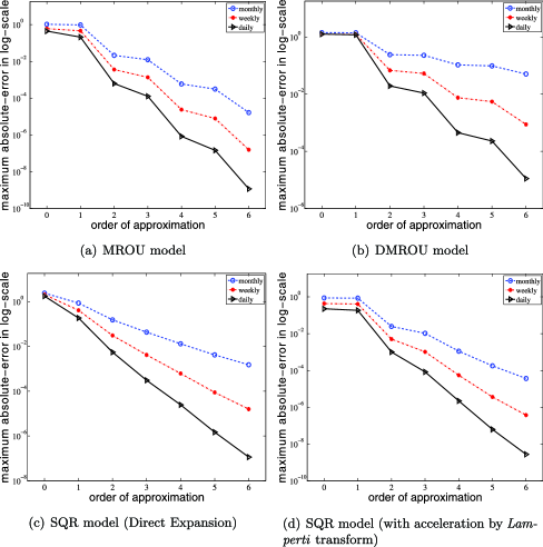
Figure 1: Maximum absolute errors of density approximation for Models 1, 2 and 3.

benchmark models (MROU, SQR and DMROU) are plotted for monthly, weekly and daily monitoring frequencies ($\Delta=1/12,1/52,1/252$) and different orders of approximation ($J=1,2,3,\ldots,6$). Especially for the SQR model, the plots are provided for both a direct expansion in Figure 1(c) and an expansion with Lamperti transform acceleration [see (32)] in Figure 1(d). Such numerical evidence demonstrates that the approximation error tends to decrease as the monitoring increment shrinks ($\Delta$ decreases) or more correction terms are included ($J$ increases), and that the combination with Lamperti transform may accelerate the convergence. As seen from the dynamics of the SQR model, the volatility function $\sigma(x)=\sigma\sqrt{x}$ violates Assumption 2 at the point $x=0$. However, the numerical performance exhibited in Figure 1(c) and (d) suggests that the technical assumptions given in Section 2 are sufficient but not necessary in order to guarantee numerical convergence of the density expansion and the resulting properties of the approximate MLE. From theoretical perspectives, the singularity at $x=0$ may lead to a significant challenge in mathematically verifying the convergence of transition density expansion, which can be regarded as a future research topic.

In the supplementary material autokey73 , we document detailed performance of the density approximation for the MROU, SQR (for both the direct expansion and the accelerated approach via Lamperti transform) and DMROU models, respectively. For the former two one-dimensional cases, that is, the MROU and SQR models, we plot the errors of approximation corresponding to weekly monitoring frequency and orders ranging from $J=1,2,\ldots,6$. For the latter set of graphs, we plot the contours of the approximation errors for the DMROU model corresponding to weekly monitoring frequency and orders ranging from $J=1,2,\ldots,6$.

The asymptotic expansion proposed in this paper is essentially different from that in Aït-Sahalia AitSahalia1999JF , AitSahalia2002Econometrica , AitSahalia2008AS and other existing large-deviations-based results. First, the expansion proposed here includes correction terms corresponding to any order of $\epsilon=\sqrt{\Delta}$; however, in Aït-Sahalia AitSahalia1999JF , AitSahalia2002Econometrica , AitSahalia2008AS and other methods, expansions include only integer orders of $\Delta$ (even orders of $\epsilon=\sqrt{\Delta}$). Second, the expansion terms in Aït-Sahalia AitSahalia1999JF , AitSahalia2002Econometrica , AitSahalia2008AS appear to be longer than the corresponding orders in the expansion proposed in this paper. Taking the MROU and the SQR model, for example, the mean-reverting correction starts from the leading order in Aït-Sahalia’s expansion; however, in our expansion, the leading order term is the density of a normal distribution, and the first appearance of mean-reverting drift parameters is deferred to the correction term corresponding to first order of $\epsilon$.

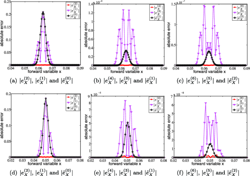
Figure 2: Cross comparisons of absolute approximation errors (corresponding to different orders of expansion) of the proposed method ($|e_{X}^{(J)}|$) and that of Aït-Sahalia AitSahalia2002Econometrica ($|\widehat{e}{}^{(J)}_{X}|$).

Let $\widehat{e}{}^{(J)}_{X}(\Delta,x|x_{0};\theta)=\widehat{p}{}^{(J)}_{X}(\Delta,x|x_{0};\theta)-p_{X}(\Delta,x|x_{0};\theta)$ denote the approximation error of Aït-Sahalia’s $J$th order expansion, where $\widehat{p}{}^{(J)}_{X}$ is defined in equation (2.14) as in Aït-Sahalia AitSahalia2002Econometrica . For the method proposed in this paper, approximation errors are denoted by $e_{X}^{(J)}(\Delta,x|x_{0};\theta)=p_{X}^{(J)}(\Delta,x|x_{0};\theta)-p_{X}(\Delta,x|x_{0};\theta)$. Without loss of generality, I employ the MROU and the SQR models to numerically illustrate the comparison of errors resulting from the method of Aït-Sahalia AitSahalia1999JF , AitSahalia2002Econometrica , AitSahalia2008AS and those from this paper. Considering different expressions and arrangements of correction terms, I make a cross comparison of absolute errors for different orders from the two methods as exhibited in Figure 2(a), (b) and (c) for the MROU model as well as Figure 2(d), (e) and (f) for the SQR model. In particular, we consider the Lamperti transform acceleration for the SQR model in order to parallel the method in Aït-Sahalia AitSahalia2002Econometrica . In the comparison, the orders range from $J=1,2,3,\ldots,6$ for our method, while $J=0,1,2$ for that of Aït-Sahalia AitSahalia2002Econometrica . Without loss of generality, the monitoring frequency is chosen as $\Delta=1/52$. As we will see, the absolute errors resulting from each two consecutive orders $J=2K-1$ and $J=2K$ of the expansion proposed in this paper sandwich that resulting from the order $K-1$ of the expansion proposed in Aït-Sahalia AitSahalia2002Econometrica , for $K=0,1,2$. The two methods both admit small magnitude of errors resulting from low order approximations and are comparable to each other as more correction terms are included.

5 Approximate maximum-likelihood estimation

This section is devoted to a method of approximate MLE based on the asymptotic expansion for transition density proposed in Section 3. Similar to Aït-Sahalia AitSahalia1999JF , AitSahalia2002Econometrica , AitSahalia2008AS , the $J$th order expansion of the log-density can be given by

$$l_{X}^{(J)}(\Delta,x|x_{0};\theta):=-\frac{m}{2}\log\Delta+\log\bigl{[}\det D(x_{0})\bigr{]}+\sum_{k=0}^{J}\Lambda_{k}\biggl{(}D(x_{0})\frac{x-x_{0}}{\sqrt{\Delta}}\biggr{)}\epsilon^{k}$$

for any $J=0,1,2,\ldots\,$, where the correction terms $\Lambda_{k}$ can be explicitly calculated from straightforward differentiation of the density expansion (3.2).

Without loss of generality, we employ Model 1 (MROU) and Model 2 (SQR) to illustrate the convergence of uniform errors of the log-density expansions ($\max_{x\in\mathcal{D}}|l_{X}^{(J)}(\Delta,x|x_{0};\theta)-\log p_{X}(\Delta,x|x_{0};\theta)|$) in Figure 3(a) and (b) in a similar way as Figure 1(a)–(d) do for the uniform errors of density expansions. For the MROU model, Figure 3(a) shows the uniform errors of its log-density expansions. For the SQR model, Figure 3(b) plots the uniform errors of its Lamperti-transformed log-density expansions which are naturally calculated from

$$l_{X}^{(J)}(\Delta,x|x_{0};\theta):=-\log\sigma(x;\theta)+l_{Z}^{(J)}\bigl{(}\Delta,\gamma(x;\theta)|\gamma(x_{0};\theta);\theta\bigr{)},$$ (33)

where $\gamma$ is the Lamperti transform and $Z(t)=\gamma(X(t);\theta)$.

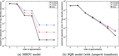
Figure 3: Maximum absolute errors of log-density approximation for Models 1 and 2.

By analogy to the log-likelihood function $\ell_{n}(\theta)$ in (3), we introduce the $J$th order approximate log-likelihood function

$$\ell_{n}^{(J)}(\theta)=\sum_{i=1}^{n}L_{i}^{(J)}(\theta),$$ (34)

where $L_{i}^{(J)}(\theta)=l_{X}^{(J)}(\Delta,X(i\Delta)|X((i-1)\Delta);\theta)$. According to Assumption 3, we assume, for simplicity, that the true log-likelihood function $\ell_{n}(\theta)$ admits a unique maximizer $\widehat{\theta}_{n}$, which serves as the true maximum-likelihood estimator. Similarly, let $\widehat{\theta}{}^{(J)}_{n}$ be the approximate maximum-likelihood estimator of order $J$ obtained from maximizing $\ell_{n}^{(J)}(\theta)$. Setting up or refining technical conditions for ensuring the identification and the usual asymptotic properties of the true but generally incomputable MLE is beyond the scope of this paper, and can be investigated as a future research topic; see, for example, Aït-Sahalia AitSahalia2002Econometrica for the discussion of one-dimensional cases. As a consequence of Theorem 2, we set up the convergence of the approximate MLE $\widehat{\theta}{}^{(J)}_{n}$ to the true MLE $\widehat{\theta}_{n}$ in what follows.

Proposition 1

Under Assumptions 1 and 2, the approximate maximum-likelihood estimator obtained from optimizing (34) satisfies that, for the fixed sample size $n$,

$$\widehat{\theta}{}^{(J)}_{n}-\widehat{\theta}_{n}\stackrel{{\scriptstyle P}}{{\rightarrow}}0$$ (35)

as $\Delta\rightarrow 0$ for $J\geq m$.

See Appendix B.

Though the convergence in (35) is theoretically justified as the monitoring increment $\Delta$ shrinks to $0$ for any fixed order $J$, the convergence of (35) may also hold as $J\rightarrow\infty$ for a range of fixed values of $\Delta$. This is analogous to the Taylor expansion in classical calculus. The respective effects on the discrepancy between the approximate MLE and the true MLE resulting from shrinking $\Delta$ and increasing expansion orders $J$ are illustrated via Monte Carlo evidence in Section 6. In particular, we will demonstrate numerically that for an arbitrary $\Delta$, a larger order $J$ results in a better approximation of the MLE.

6 Monte Carlo evidence of approximate maximum-likelihood estimation

To further demonstrate the convergence issues discussed in the previous sections, we provide Monte Carlo evidence of approximate maximum-likelihood estimation for the three models discussed in Section 4. Let $N$ denote the number of sample paths generated from the transition distributions; let $n$ denote the number of observations on each path. For finite-sample results, we report the mean and standard deviation of the discrepancy between the MLE and the true parameter value (i.e., $\widehat{\theta}_{n}-\theta^{\mathrm{True}}$), and the discrepancy between the approximate MLE and the MLE (i.e., $\widehat{\theta}{}^{(J)}_{n}-\widehat{\theta}_{n}$).

For the two Gaussian models, that is, the MROU model and the DMROU model, the situation considered here is restricted to the stationary case. Therefore, the asymptotic variance of the maximum-likelihood estimator is given by the inverse of Fisher’s information matrix, which is the lowest possible variance of all estimators. So, as in Aït-Sahalia AitSahalia1999JF , AitSahalia2002Econometrica , AitSahalia2008AS , we assume that $\kappa>0$ for the MROU model, and $\kappa_{11}>0$ and $\kappa_{22}>0$ for the DMROU model. By the nature of stationarity, one has the local asymptotic normal structure for the maximum-likelihood estimator $\widehat{\theta}_{n}$, that is,

$$\sqrt{n}(\widehat{\theta}_{n}-\theta)\stackrel{{\scriptstyle\mathcal{D}}}{{\rightarrow}}\mathcal{N}\bigl{(}0,i(\theta)^{-1}\bigr{)}$$ (36)

as $n\rightarrow\infty$ with $\Delta$ fixed. Here, the Fisher information matrix is calculated as

$$i(\theta)=-\mathbb{E}\biggl{(}\frac{\partial^{2}L_{1}(\theta)}{\partial\theta\,\partial\theta^{T}}\biggr{)},$$ (37)

where ^T denotes matrix transposition.

Table 1: Monte Carlo evidence for the MROU model

	Asymptotic		Finite sample		Finite sample		Finite sample
Parameters $\bolds{\theta^{\mathrm{True}}}$	$\bolds{\widehat{\theta}_{n}-\theta^{\mathrm{True}}}$		$\bolds{\widehat{\theta}_{n}-\theta^{\mathrm{True}}}$		$\bolds{\widehat{\theta}{}^{(3)}_{n}-\widehat{\theta}_{n}}$		$\bolds{\widehat{\theta}{}^{(6)}_{n}-\widehat{\theta}_{n}}$
	Mean	Stddev	Mean	Stddev	Mean	Stddev	Mean	Stddev
$\Delta=1/52$
$\kappa=0.5$	0	0.229136	0.245175	0.329396	0.013477	0.014645	$0.000002$	0.000102
$\alpha=0.06$	0	0.013682	0.000329	0.015202	0.000002	0.000318	$0.000000$	0.000003
$\sigma=0.03$	0	0.000674	0.000021	0.000675	0.000003	0.000015	$-0.000000$	0.000000
$\Delta=1/12$
$\kappa=0.5$	0	0.111867	0.054162	0.124773	0.028923	0.014382	$-0.000003$	0.000297
$\alpha=0.06$	0	0.006573	0.000097	0.006440	0.000002	0.000174	$0.000000$	0.000014
$\sigma=0.03$	0	0.000685	0.000022	0.000687	0.000025	0.000022	$0.000000$	0.000001

[]Notes. The number of simulation trials is $N=5000$ and the number of observations on each path is $n=1000$.

Without loss of generality, we analyze the results of the MROU model in what follows. As seen from Table 1, the asymptotic distribution of $\widehat{\theta}_{n}-\theta^{\mathrm{True}}$ is calculated from (36) and (37). The small discrepancy between the finite-sample and asymptotic standard deviations of $\widehat{\theta}_{n}-\theta^{\mathrm{True}}$ indicates that the choice of sample size $n=1000$ is approaching an optimality. When the monitoring frequency $\Delta$ shrinks, or when the order of approximation $J$ increases, the approximate MLEs obtained from maximizing the approximate log-likelihood function (34) get closer to the exact (but usually incomputable) MLEs, and thus get closer to the true parameter, if the sample size $n$ is large enough. This can be seen by a comparison of some outputs with relatively larger bias and standard deviations resulting from relatively lower order expansions or larger monitoring increments with those improved outputs resulting from relatively higher order expansions and smaller monitoring increments. This phenomenon reconciles our discussions in Section 5.

While holding the length of sampling interval $\Delta$ fixed, the approximation error $\widehat{\theta}{}^{(J)}_{n}-\widehat{\theta}_{n}$ decreases and is dominated by the intrinsic sampling error $\widehat{\theta}_{n}-\theta^{\mathrm{True}}$ as $J$ increases. Therefore, according to Aït-Sahalia AitSahalia1999JF , AitSahalia2002Econometrica , AitSahalia2008AS , a small-order approximation (e.g., the $\widehat{\theta}{}^{(6)}_{n}$ for the MROU model) is adequate enough for replacing the true MLE $\widehat{\theta}_{n}$ for the purpose of estimating unknown parameter $\theta$. According to Aït-Sahalia AitSahalia1999JF , AitSahalia2002Econometrica , AitSahalia2008AS , once the approximation error resulting from replacing the true density $p_{X}$ by its approximation, say $p_{X}^{(J)}$, is dominated by the sampling error [usually estimated from asymptotic variance computed from (36)] due to the true maximum-likelihood estimation, such $p_{X}^{(J)}$ is appropriate in practice. Such a proper replacement has an effect that is statistically indiscernible from the sampling variation of the true yet incomputable MLE $\widehat{\theta}_{n}$ around $\theta$. As a result of the fast development of modern computation and optimization technology, calculation of high-order likelihood approximations will become increasingly feasible; thus errors between approximate MLE and MLE can be improved to become arbitrarily small, at least in principle.

Owing to the limited space in this paper and the similarity in the pattern of results to those of the MROU model, we collect the simulation results for the DMROU and the SQR models in the supplementary material autokey73 . In particular, for the SQR model, the simulation results will demonstrate that a combination of the Lamperti transform and our expansion may enhance the efficiency of the estimation. Moreover, in the supplementary material autokey73 , we will investigate two more sophisticated data-generating processes (arising from financial modeling) with rich drift and diffusion specifications, in which the Lamperti transform either requires computationally demanding implicit integration and inversion or does not exist due to a multivariate irreducible specification; see Aït-Sahalia AitSahalia2008AS .

7 Concluding remarks

This paper contributes a method for approximate maximum-likelihood estimation (MLE) of multivariate diffusion processes from discretely sampled data, based on a closed-form asymptotic expansion for transition density, for which any arbitrary order of corrections can be systematically obtained through a generally implementable algorithm. Numerical examples and Monte Carlo evidence for illustrating the performance of density asymptotic expansion and the resulting approximate MLE are provided in order to demonstrate the wide applicability of the method. Based on some sufficient (but not necessary) technical conditions, the convergence and asymptotic properties are theoretically justified. Owing to the limited space of this paper which focuses on introducing a method of estimation, investigations on more asymptotic properties related to the approximate MLE can be regarded as a future research topic, for example, a tighter upper bound for the discrepancy (35) based on the error estimate of the transition density expansion (31), as well as the consistency and asymptotic distribution of the approximate MLE under various sampling schemes in terms of monitoring frequency and observational horizon; see, for example, Yoshida Yoshida1992Discrete , Kessler Kessler1997 , Bibby and Sørensen BibbySorensen1995 and Genon-Catalot and Jacod GenonCatalotJacod1993 . In this regard, we note Chang and Chen ChangChen2011 for analyzing the asymptotic properties of the approximate MLE proposed in Aït-Sahalia AitSahalia2002Econometrica of one-dimensional diffusion processes. One may also apply the idea for explicitly approximating transition density in various other aspects of statistical inference, for which explicit asymptotic expansions of certain quantities are helpful.

Appendix A Explicit calculation of conditional expectation (28)

In this section, we expatiate on a general algorithm for explicitly calculating the conditional expectation (28) of multiplication of iterated Stratonovich integrals as a multivariate polynomial in $z=(z_{1},z_{2},\ldots,z_{m})\in\mathbb{R}^{m}$. In addition to theoretical interests, iterated stochastic integral plays important roles in many applications arising from stochastic modeling, for example, the analysis of convergence rate of various methods for approximating solutions to stochastic differential equations; see Kloeden and Platen KloedenPlaten1999 . Special cases for conditional expectations of iterated Itô stochastic integrals (without integral with respect to the time variable) can be found in, for example, Nualart, Üstünel and Zakai NualartUstunelZakai1988 , Yoshida Yoshida1992StatisticsSmallDiffusion , Yoshida1992MLE and Kunitomo and Takahashi KunitomoTakahashi2001mathfinance .

To present our algorithm, similar to the definition of iterated Stratonovich integral, we define

$$\quad I_{\mathbf{i}}[f](t):=\int_{0}^{t}\int_{0}^{t_{1}}\cdots\int_{0}^{t_{n-1}}f(t_{n})\,dW_{i_{n}}(t_{n})\cdots dW_{i_{2}}(t_{2})\,dW_{i_{1}}(t_{1})$$ (38)

as an iterated Itô integral for an arbitrary index $\mathbf{i}=(i_{1},i_{2},\break\ldots,i_{n})\in\{0,1,2,\ldots,m\}^{n}$ with a right-continuous integrand $f$. To lighten the notation, the integral $I_{\mathbf{i}}[1](t)$ is abbreviated to $I_{\mathbf{i}}(t)$.

Before discussing details in the following subsections, we briefly outline a general algorithm, which can be implemented using any symbolic packages, for example, Mathematica. Throughout our discussion, the iterated (Stratonovich or Itô) stochastic integrals may involve integrations with respect to not only Brownian motions but also time variables.

• Convert each iterated Stratonovich integral in (28) to a linear combination of iterated Itô integrals;

• Convert each multiplication of iterated Itô integrals resulting from the previous step to a linear combination of iterated Itô integrals;

• Compute the conditional expectation of iterated Itô integral via an explicit construction of Brownian bridge.

A.1 Conversion from iterated Stratonovich integrals to Itô integrals

Denote by $l(\mathbf{i}):=l((i_{1},\ldots,i_{n}))=n$ the length of the index $\mathbf{i}$. Denote by $-\mathbf{i}$ an index obtained from deleting the first element of $\mathbf{i}$. In particular, if $l(\mathbf{i})=0$, we define $J_{\mathbf{i}}[f](t)=f(t)$ by slightly extending the definition (9). According to page 172 of Kloeden and Platen KloedenPlaten1999 , we have the following conversion algorithm: for the case of $l(\mathbf{i})=0$ or $1$, we have $J_{\mathbf{i}}(t)=I_{\mathbf{i}}(t)$; for the case of $l(\mathbf{i})\geq 2$, we have

$$J_{\mathbf{i}}(t)=I_{(i_{1})}\bigl{[}J_{-\mathbf{i}}(\cdot)\bigr{]}(t)+1_{\{i_{1}=i_{2}\neq 0\}}I_{(0)}\bigl{[}\tfrac{1}{2}J_{-(-\mathbf{i})}(\cdot)\bigr{]}(t).$$ (39)

For example, if $l(\mathbf{i})=2$, one has

$${J_{\mathbf{i}}(t)=I_{{}_{\mathbf{i}}}(t)+\tfrac{1}{2}1}_{{\{i_{1}=i_{2}\neq 0\}}}{I_{(0)}(t).}$$

Thus, with the conversion algorithm (39), we convert each iterated Stratonovich integral in (28) to a linear combination of iterated Itô integrals. Thus, the product $\prod_{\omega=1}^{l}J_{\mathbf{i}_{\omega}}(1)$ can be expanded as a linear combination of multiplication of Itô integrals.

A.2 Conversion from multiplication of Itô integrals to a linear combination

We provide a simple recursion algorithm for converting a multiplication of iterated Itô integrals to a linear combination. According to Lemma 2 in Tocino Tocino2009 , a product of two Itô integrals as defined in (38) satisfies that

$$I_{\bolds{\alpha}}(t)I_{\bolds{\beta}}(t) = \int_{0}^{t}I_{\bolds{\alpha}}(s)I_{-\bolds{\beta}}(s)\,dW_{\beta_{1}}(s)+\int_{0}^{t}I_{-\bolds{\alpha}}(s)I_{\bolds{\beta}}(s)\,dW_{\alpha_{1}}(s)$$

$${}+\int_{0}^{t}I_{-\bolds{\alpha}}(s)I_{-\bolds{\beta}}(s)1_{\{\alpha_{1}=\beta_{1}\neq 0\}}\,ds$$

for any arbitrary indices $\bolds{\alpha}=(\alpha_{1},\alpha_{2},\ldots,\alpha_{p})$ and $\bolds{\beta}=(\beta_{1},\beta_{2},\ldots,\beta_{q})$. Iterative applications of this relation render a linear combination form of $I_{\bolds{\alpha}}(t)I_{\bolds{\beta}}(t)$. Inductive applications of such an algorithm convert a product of any number of iterated Itô integrals to a linear combination. Therefore, our immediate task is reduced to the calculation of conditional expectations of iterated Itô integrals.

A.3 Conditional expectation of iterated Itô integral

We focus on the explicit calculation of conditional expectations of the following type:

$$\mathbb{E}\bigl{(}I_{\mathbf{i}}(1)|W(1)=z\bigr{)}$$

$$\qquad=\mathbb{E}\biggl{(}\int_{0}^{1}\int_{0}^{t_{1}}\cdots\int_{0}^{t_{n-1}}dW_{i_{n}}({t_{n})}\cdots dW_{i_{2}}(t_{2})\,dW_{i_{1}}(t_{1})|W(1)=z\biggr{)}.$$

By an explicit construction of Brownian bridge (see page 358 in Karatzas and Shreve KaraztasShreve ), we obtain the following distributional identity, for any $k=1,2,\ldots,m$:

$$\bigl{(}W_{k}(t)|W(1)=z\bigr{)}\stackrel{{\scriptstyle\mathcal{D}}}{{=}}\bigl{(}W_{k}(t)|W_{k}(1)=z_{k}\bigr{)}\stackrel{{\scriptstyle\mathcal{D}}}{{=}}BB_{k}^{z}(t):=\mathcal{B}_{k}(t)-t\mathcal{B}_{k}(1)+tz_{k},$$

where $\mathcal{B}_{k}$’s are independent Brownian motions and $BB_{k}^{z}(t):=\mathcal{B}_{k}(t)-t\mathcal{B}_{k}(1)+tz_{k}$ is distributed as a Brownian bridge starting from $0$ and ending at $z_{k}$ at time $1$. For ease of exposition, we also introduce $\mathcal{B}_{0}(t)\equiv 0$ and $z_{0}=1$. Therefore, the condition $W(1)=z$ in (A.3) can be eliminated since

$$\mathbb{E}\biggl{(}\int_{0}^{1}\int_{0}^{t_{1}}\cdots\int_{0}^{t_{n-1}}dW_{i_{n}}({t_{n})}\cdots dW_{i_{2}}(t_{2})\,dW_{i_{1}}(t_{1})|W(1)=z\biggr{)}$$

$$\qquad=\mathbb{E}\biggl{(}\int_{0}^{1}\int_{0}^{t_{1}}\cdots\int_{0}^{t_{n-1}}d\bigl{(}\mathcal{B}_{i_{n}}(t_{n})-t_{n}\mathcal{B}_{i_{n}}(1)+t_{n}z_{i_{n}}\bigr{)}\cdots$$

(42)

$$\hskip 121.7ptd\bigl{(}\mathcal{B}_{i_{2}}(t_{2})-t_{2}\mathcal{B}_{i_{2}}(1)+t_{2}z_{i_{2}}\bigr{)}$$

$$\hskip 140.0ptd\bigl{(}\mathcal{B}_{i_{1}}(t_{1})-t_{1}\mathcal{B}_{i_{1}}(1)+t_{1}z_{i_{1}}\bigr{)}\biggr{)}.$$

An early attempt using the idea of Brownian bridge to deal with conditional expectation (A.3) can be found in Uemura Uemura1987 , which investigated the calculation of heat kernel expansion in the diagonal case. It is worth mentioning that, instead of giving a method for explicitly calculating (A.3), Uemura Uemura1987 employed discretization of stochastic integrals to show that (A.3) has the structure of a multivariate polynomial in $z$ with unknown coefficients. Therefore, the validity of the above derivation can be seen from the definition of stochastic integral as a limit of discretized summation. In particular, the random variables $\mathcal{B}_{i_{1}}(1),\mathcal{B}_{i_{2}}(1),\ldots,\mathcal{B}_{i_{n}}(1)$ are not involved in the integral in (A.3). The integrals with respect to $d\mathcal{B}_{i_{k}}(t_{k})$ are in the sense of usual stochastic integrals; the integrals with respect to $dt_{k}$ are in the sense of Lebesgue integrals.

By expanding the right-hand side of (A.3) and collecting terms according to monomials of $z_{i}$’s, we express (A.3) as a multivariate polynomial in $z$:

$$\mathbb{E}\bigl{(}I_{\mathbf{i}}(1)|W(1)=z\bigr{)}=\sum_{k=0}^{n}\sum_{\{l_{1},l_{2},\ldots,l_{k}\}\subset\{1,2,\ldots,n\}}c(l_{1},l_{2},\ldots,l_{k})z_{i_{l_{1}}}z_{i_{l_{2}}}\cdots z_{i_{l_{k}}},$$

where the coefficients are determined by

$$c(l_{1},l_{2},\ldots,l_{k})$$

$$\qquad:=\mathbb{E}\int_{0}^{1}\int_{0}^{t_{1}}\cdots\int_{0}^{t_{n-1}}d\bigl{(}\mathcal{B}_{i_{n}}(t_{n})-t_{n}\mathcal{B}_{i_{n}}(1)\bigr{)}\cdots$$

$$\qquad\hskip 97.0ptd\bigl{(}\mathcal{B}_{i_{l_{k}+1}}(t_{l_{k}+1})-t_{l_{k}+1}\mathcal{B}_{i_{l_{k}+1}}(1)\bigr{)}$$

$$\qquad\hskip 97.0ptdt_{l_{k}}\,d\bigl{(}\mathcal{B}_{i_{l_{k}-1}}(t_{l_{k}-1})-t_{l_{k}-1}\mathcal{B}_{i_{l_{k}-1}}(1)\bigr{)}\cdots$$

(43)

$$\qquad\hskip 97.0ptd\bigl{(}\mathcal{B}_{i_{l_{2}+1}}(t_{l_{2}+1})-t_{l_{2}+1}\mathcal{B}_{i_{l_{2}+1}}(1)\bigr{)}$$

$$\qquad\hskip 97.0ptdt_{l_{2}}\,d\bigl{(}\mathcal{B}_{i_{l_{2}-1}}(t_{l_{2}-1})-t_{l_{2}-1}\mathcal{B}_{i_{l_{2}-1}}(1)\bigr{)}\cdots$$

$$\qquad\hskip 97.0ptd\bigl{(}\mathcal{B}_{i_{l_{1}+1}}(t_{l_{1}+1})-t_{l_{1}+1}\mathcal{B}_{i_{l_{1}+1}}(1)\bigr{)}$$

$$\qquad\hskip 97.0ptdt_{l_{1}}\,d\bigl{(}\mathcal{B}_{i_{l_{1}-1}}(t_{l_{1}-1})-t_{l_{1}-1}\mathcal{B}_{i_{l_{1}-1}}(1)\bigr{)}\cdots$$

$$\qquad\hskip 97.0ptd\bigl{(}\mathcal{B}_{i_{1}}(t_{1})-t_{1}\mathcal{B}_{i_{1}}(1)\bigr{)}.$$

Algebraic calculation from expanding the terms like $d(\mathcal{B}_{i_{n}}(t_{n})-t_{n}\mathcal{B}_{i_{n}}(1))$ simplifies (A.3) as a linear combination of expectations of the following form: $\mathbb{E}(\mathcal{B}_{m_{1}}(1)\mathcal{B}_{m_{2}}(1)\cdots\mathcal{B}_{m_{r}}(1)I_{\mathbf{j}}(1))$ where $I_{\mathbf{j}}(1)$ is an iterated Itô integral.

By viewing $\mathcal{B}_{m_{i}}(1)$ as $\int_{0}^{1}d\mathcal{B}_{m_{i}}(t_{1})$, we have

$$\mathbb{E}\bigl{(}\mathcal{B}_{m_{1}}(1)\mathcal{B}_{m_{2}}(1)\cdots\mathcal{B}_{m_{r}}(1)I_{\mathbf{j}}(1)\bigr{)}=\mathbb{E}\Biggl{(}\prod_{i=1}^{r}\int_{0}^{1}d\mathcal{B}_{m_{i}}(t_{1})I_{\mathbf{j}}(1)\Biggr{)}.$$ (44)

To calculate this expectation, we use the algorithm proposed in Section A.2 to convert $\prod_{i=1}^{r}\int_{0}^{1}d\mathcal{B}_{m_{i}}(t_{1})I_{\mathbf{j}}(1)$ to a linear combination of iterated Itô integrals. Finally, we need to calculate expectation of iterated Itô integrals without conditioning. For any arbitrary index $\mathbf{i}=(i_{1},i_{2},\ldots,i_{n})\in\{0,1,2,\ldots,m\}^{n}$, we have

$$\mathbb{E}I_{\mathbf{i}}(1) = \mathbb{E}\biggl{(}\int_{0}^{1}\int_{0}^{t_{1}}\cdots\int_{0}^{t_{n-1}}dW_{i_{n}}({t_{n})}\cdots dW_{i_{2}}(t_{2})\,dW_{i_{1}}(t_{1})\biggr{)}$$

$$= \int_{0}^{1}\int_{0}^{t_{1}}\cdots\int_{0}^{t_{n-1}}d{t_{n}}\cdots dt_{2}\,dt_{1}\equiv\frac{1}{n!},$$

if $\mathbf{i}=(i_{1},i_{2},\ldots,i_{n})=(0,0,\ldots,0)$ and $\mathbb{E}I_{\mathbf{i}}(1)=0$, otherwise (by the martingale property of stochastic integrals).

Appendix B Proofs

B.1 Proof of Theorem 1

Using the chain rule and the Taylor theorem, the $k$th ($k\geq 1$) order correction term for $\delta(Y^{\epsilon}-y)$ admits the following form:

$$\Phi_{k}(y) = \sum_{(l,\mathbf{r}(l),\mathbf{j}(l))\in S_{k}}\,\frac{1}{l!}\partial^{\mathbf{r}}\delta\bigl{(}B(1)-y\bigr{)}Y_{j_{1},r_{1}}Y_{j_{2},r_{2}}\cdots Y_{j_{l},r_{l}},$$ (45)

where $\partial^{\mathbf{r}}$ denotes $\frac{\partial}{\partial x_{r_{1}}}\,\frac{\partial}{\partial x_{r_{2}}}\cdots\frac{\partial}{\partial x_{{}_{{}^{r_{l}}}}}$ for simplicity. Thus, taking expectation of (45) and applying (22), we obtain that

$$\Omega_{k}(y) = \mathbb{E}\Phi_{k}(y)$$

$$= \sum_{(l,\mathbf{r}(l),\mathbf{j}(l))\in S_{k}}\frac{1}{l!}D_{r_{1}r_{1}}(x_{0})D_{r_{2}r_{2}}(x_{0})\cdots D_{r_{l}r_{l}}(x_{0})$$

$$\hskip 52.0pt{}\times\mathbb{E}\bigl{(}\partial^{\mathbf{r}}\delta\bigl{(}B(1)-y\bigr{)}F_{j_{1}+1,r_{1}}F_{j_{2}+1,r_{2}}\cdots F_{j_{l}+1,r_{l}}\bigr{)}.$$

Employing the integration-by-parts property of the Dirac delta function (see, e.g., Section 2.6 in Kanwal Kanwal2004generalizedfunctions ), the conditional expectation can be computed as

$$\mathbb{E}\bigl{[}\partial^{\mathbf{r}}\delta\bigl{(}B(1)-y\bigr{)}F_{j_{1}+1,r_{1}}F_{j_{2}+1,r_{2}}\cdots F_{j_{l}+1,r_{l}}\bigr{]}$$

$$\qquad=\int_{b\in\mathbb{R}^{d}}\mathbb{E\bigl{[}}\partial^{\mathbf{r}}\delta\bigl{(}B(1)-y\bigr{)}F_{j_{1}+1,r_{1}}F_{j_{2}+1,r_{2}}\cdots F_{j_{l}+1,r_{l}}|B(1)=b\bigr{]}$$

$$\hskip 23.5pt\qquad\quad{}\times\phi_{\Sigma(x_{0})}(b)\,db$$

$$\qquad=(-1)^{l}\,\partial^{\mathbf{r}}\bigl{[}\mathbb{E\bigl{[}}F_{j_{1}+1,r_{1}}F_{j_{2}+1,r_{2}}\cdots F_{j_{l}+1,r_{l}}|W(1)=\sigma(x_{0})^{-1}D(x_{0})^{-1}y\bigr{]}$$

$$\qquad\hskip 256.0pt{}\times\phi_{\Sigma(x_{0})}(y)\bigr{]},$$

where $\phi_{\Sigma(x_{0})}(y)$ is given in (3.2). By plugging in (14), we have that

$$\mathbb{E}\bigl{[}F_{j_{1}+1,r_{1}}F_{j_{2}+1,r_{2}}\cdots F_{j_{l}+1,r_{l}}|W(1)=z\bigr{]}$$

$$\qquad=\sum_{\{(\mathbf{i}_{1},\mathbf{i}_{2},\ldots,\mathbf{i}_{l})|\|\mathbf{i}_{\omega}\|=j_{\omega}+1,\omega=1,2,\ldots,l\}}\prod_{\omega=1}^{l}C_{\mathbf{i}_{\omega},r_{\omega}}(x_{0})P_{(\mathbf{i}_{1},\mathbf{i}_{2},\ldots,\mathbf{i}_{l})}(z),$$

where $P_{(\mathbf{i}_{1},\mathbf{i}_{2},\ldots,\mathbf{i}_{l})}(z)$ is defined in (28). Formula (29) follows from the fact that

$$\frac{\partial}{\partial y_{i}}\bigl{(}P_{(\mathbf{i}_{1},\mathbf{i}_{2},\ldots,\mathbf{i}_{l})}\bigl{(}\sigma(x_{0})^{-1}D(x_{0})^{-1}y\bigr{)}\phi_{\Sigma(x_{0})}(y)\bigr{)}$$

$$\qquad=\biggl{(}\frac{\partial}{\partial y_{i}}P_{(\mathbf{i}_{1},\mathbf{i}_{2},\ldots,\mathbf{i}_{l})}\bigl{(}\sigma(x_{0})^{-1}D(x_{0})^{-1}y\bigr{)}$$

$$\hskip 5.2pt\qquad\quad{}-P_{(\mathbf{i}_{1},\mathbf{i}_{2},\ldots,\mathbf{i}_{l})}\bigl{(}\sigma(x_{0})^{-1}D(x_{0})^{-1}y\bigr{)}\bigl{(}\Sigma(x_{0})^{-1}y\bigr{)}_{i}\biggr{)}\phi_{\Sigma(x_{0})}(y)$$

as well as the definition of the differential operators in (18).

Remark 1.

The above conditioning argument can be justified, when $\partial^{\mathbf{r}}\delta(B(1)-y)$ is regarded as a generalized Wiener functional (random variable) and the expectation is interpreted in the corresponding generalized sense as in Watanabe WatanabeAnalysisofWiener1987 .

B.2 Proof of Theorem 2

Now, based on Assumption 2, we introduce the following uniform upper bounds. For $k\geq 1$, let $\mu_{k}$ and $\sigma_{k}$ be the uniform upper bounds of the $k$th order derivative of $\mu$ and $\sigma$, respectively, that is,

$$\biggl{|}\frac{\partial^{(k)}\mu(x;\theta)}{\partial x^{k}}\biggr{|}\leq\mu_{k}\quad\mbox{and}\quad\biggl{|}\frac{\partial^{(k)}\sigma(x;\theta)}{\partial x^{k}}\biggr{|}\leq\sigma_{k}$$ (46)

for $(x,\theta)\in\mathbb{R}^{m}\times\Theta$. Also, let $\mu_{0}$ and $\sigma_{0}$ denote the uniform upper bounds of $|\mu(x_{0};\theta)|$ and $|\sigma(x_{0};\theta)|$ on $(x_{0},\theta)\in K\times\Theta$, respectively, that is,

$$\bigl{|}\mu(x_{0};\theta)\bigr{|}\leq\mu_{0}\quad\mbox{and}\quad\bigl{|}\sigma(x_{0};\theta)\bigr{|}\leq\sigma_{0}$$ (47)

for $(x_{0},\theta)\in K\times\Theta$. In order to establish the uniform convergence in Theorem 2, we introduce the following lemma. When the dependence of parameters is emphasized, we express $X^{\epsilon}(1)$ as $X^{\epsilon}(1;\theta,x_{0})$ and express the standardized random variable $Y^{\epsilon}$ defined in (20) as

$$Y^{\epsilon}(\theta,x_{0})=D(x_{0})\bigl{(}X^{\epsilon}(1;\theta,x_{0})-x_{0}\bigr{)}/\sqrt{\Delta}.$$

In this Appendix, we employ standard notation of Malliavin calculus (see, e.g., Nualart NualartMCbook and Ikeda and Watanabe IkedaWatanabe1989 ) and the theory of Watanabe WatanabeAnalysisofWiener1987 and Yoshida Yoshida1992StatisticsSmallDiffusion , Yoshida1992MLE . For the readers’ convenience, a brief survey of some relative theory is provided in the supplementary material autokey73 .

Lemma 2

Under Assumption 2, the pathwise expansion (22) holds in the sense of $D^{\infty}$ uniformly in $(x_{0},\theta)\in K\times\Theta$, that is,

$$\Biggl{\|}Y^{\epsilon}(\theta,x_{0})-\sum_{k=0}^{J}\frac{1}{k!}\,\frac{\partial^{(k)}Y^{\epsilon}(\theta,x_{0})}{\partial\epsilon^{k}}\bigg{|}_{\epsilon=0}\epsilon^{k}\Biggr{\|}_{D_{p}^{s}}=\mathcal{O}\bigl{(}\epsilon^{J+1}\bigr{)}$$

for any $J\in\mathbb{N}$, $p\geq 1$ and $s\in\mathbb{N}$.

See the supplementary material autokey73 .

Because of Assumption 1, Theorem 3.4 in Watanabe WatanabeAnalysisofWiener1987 guarantees the uniform nondegenerate condition, that is,

$$\limsup_{\epsilon\rightarrow 0}\mathbb{E}\bigl{[}\det\bigl{(}\Sigma\bigl{(}Y^{\epsilon}(\theta,x_{0})\bigr{)}\bigr{)}^{-p}\bigr{]}<\infty\qquad\mbox{for any }p\in(0,+\infty).$$

Let $\Lambda=\mathbb{R}^{m}$ denote a set of indices. For any $y=(y_{1},\ldots,y_{m})\in\Lambda$, let us consider a generalized function defined as $T_{y}(z):=\delta(z-y)$, which is a Schwartz distribution, that is, $T_{y}\in\mathcal{S}^{\prime}(\mathbb{R}^{m})$. Applying Theorem 2.3 in Watanabe WatanabeAnalysisofWiener1987 and Theorem 2.2 in Yoshida Yoshida1992MLE , we obtain that $T_{y}(Y^{\epsilon}(\theta,x_{0}))$ admits the following asymptotic expansion: for any arbitrary $J\in\mathbb{N}$,

$$\delta\bigl{(}Y^{\epsilon}(\theta,x_{0})-y\bigr{)}:=\sum_{k=0}^{J}\Phi_{k,(\theta,x_{0})}(y)\epsilon^{k}+\mathcal{O}\bigl{(}\epsilon^{J+1}\bigr{)}\qquad\mbox{in }D^{-\infty},$$

uniform in $y\in\Lambda$, $x_{0}\in K$ and $\theta\in\Theta$. Here, the correction term $\Phi_{k,(\theta,x_{0})}(y)$ is given in (45). Therefore, we obtain that

$$\sup_{y\in\Lambda,x_{0}\in K,\theta\in\Theta}\Biggl{|}\mathbb{E}\Biggl{(}\delta\bigl{(}Y^{\epsilon}(\theta,x_{0})-y\bigr{)}-\sum_{k=0}^{J}\Phi_{k,(\theta,x_{0})}(y)\epsilon^{k}\Biggr{)}\Biggr{|}=\mathcal{O}\bigl{(}\epsilon^{J+1}\bigr{)}.$$

Hence, by taking into account the transform (20), we obtain that

$$\mathop{\sup_{(x,x_{0},\theta)}}_{\in E\times K\times\Theta}\Biggl{|}\mathbb{E}\delta\bigl{(}X^{\epsilon}(1)-x\bigr{)}-\frac{\det D(x_{0})}{\sqrt{\Delta^{m}}}\sum_{k=0}^{J}\Omega_{k}\biggl{(}\frac{D(x_{0})(x-x_{0})}{\sqrt{\Delta}}\biggr{)}\epsilon^{k}\Biggr{|}$$

$$\qquad=\mathcal{O}\bigl{(}\Delta^{({J+1-m})/{2}}\bigr{)},$$

which yields (31).

B.3 Proof of Proposition 1

For $J\geq m$, let

$$R^{(J)}(\Delta,x|x_{0};\Theta):=\sup_{\theta\in\Theta}\bigl{|}p_{X}(\Delta,x|x_{0};\theta)-p_{X}^{(J)}(\Delta,x|x_{0};\theta)\bigr{|}.$$

By Theorem 2, there exists a constant $C>0$ such that $R^{(J)}(\Delta,x|x_{0};\Theta)\leq C\epsilon^{J+1-m}$ for any $x\in E$ and $\epsilon$ sufficiently small. Thus, for any positive integer $k$, it follows that

$$\mathbb{E}\bigl{[}\bigl{|}R^{(J)}\bigl{(}\Delta,X(t+\Delta)|X(t);\Theta\bigr{)}\bigr{|}^{k}|X(t)=x_{0}\bigr{]}\leq C^{k}\epsilon^{k(J+1-m)}\rightarrow 0\qquad\mbox{as }\epsilon\rightarrow 0.$$

By the Chebyshev inequality, $R^{(J)}(\Delta,X(t+\Delta)|X(t);\Theta)$ converges to zero in probability given $X(t)=x_{0}$, that is, for any $\varepsilon>0$,

$$\mathbb{P}\bigl{[}\bigl{|}R^{(J)}\bigl{(}\Delta,X(t+\Delta)|X(t);\Theta\bigr{)}\bigr{|}>\varepsilon|X(t)=x_{0}\bigr{]}\rightarrow 0\qquad\mbox{as }\epsilon\rightarrow 0.$$

By conditioning, it follows that

$$\mathbb{P}\bigl{[}\bigl{|}R^{(J)}\bigl{(}\Delta,X(t+\Delta)|X(t);\Theta\bigr{)}\bigr{|}>\varepsilon\bigr{]}$$

$$\qquad=\int_{R}\mathbb{P}\bigl{[}\bigl{|}R^{(J)}\bigl{(}\Delta,X(t+\Delta)|X(t);\Theta\bigr{)}\bigr{|}>\varepsilon|X(t)=x_{0}\bigr{]}\mathbb{P}\bigl{(}X(t)\in dx_{0}\bigr{)}.$$

Because of the fact that

$$0\leq\mathbb{P}\bigl{[}\bigl{|}R^{(J)}\bigl{(}\Delta,X(t+\Delta)|X(t);\Theta\bigr{)}\bigr{|}>\varepsilon|X(t)=x_{0}\bigr{]}\leq 1$$

and $\int_{R}\mathbb{P}(X(t)\in dx_{0})=1$, it follows from the Lebesgue dominated convergence theorem that

$$\mathbb{P}\bigl{[}\bigl{|}R^{(J)}\bigl{(}\Delta,X(t+\Delta)|X(t);\Theta\bigr{)}\bigr{|}>\varepsilon\bigr{]}\rightarrow 0\qquad\mbox{as }\epsilon\rightarrow 0,$$

that is,

$$\mathbb{P}\Bigl{[}\sup_{\theta\in\Theta}\bigl{|}p_{X}\bigl{(}\Delta,X(t+\Delta)|X(t);\theta\bigr{)}-p_{X}^{(J)}\bigl{(}\Delta,X(t+\Delta)|X(t);\theta\bigr{)}\bigr{|}>\varepsilon\Bigr{]}\rightarrow 0$$

as $\epsilon\rightarrow 0$. Now, we obtain that

$$p_{X}^{(J)}\bigl{(}\Delta,X(t+\Delta)|X(t);\theta\bigr{)}-p_{X}\bigl{(}\Delta,X(t+\Delta)|X(t);\theta\bigr{)}\stackrel{{\scriptstyle\mathbb{P}}}{{\rightarrow}}0$$ (48)

as $\epsilon\rightarrow 0$ uniformly in $\theta\in\Theta$. Following similar lines of argument as those in the proof of Theorem 2 in Aït-Sahalia AitSahalia2002Econometrica and Theorem 3 in Aït-Sahalia AitSahalia2008AS , we arrive at

$$L_{i}^{(J)}(\theta)\stackrel{{\scriptstyle\mathbb{P}}}{{\rightarrow}}L_{i}(\theta)\qquad\mbox{as }\epsilon\rightarrow 0\mbox{ uniformly in }\theta\in\Theta$$

by the convergence in (48) and continuity of logarithm. Hence, for any arbitrary $n>0$, one obtains the convergence of log-likelihood $\ell_{n}^{(J)}(\theta)\stackrel{{\scriptstyle\mathbb{P}}}{{\rightarrow}}\ell_{n}(\theta)$ uniformly in $\theta$. Finally, the convergence of $\widehat{\theta}{}^{(J)}_{n}-\widehat{\theta}_{n}\stackrel{{\scriptstyle\mathbb{P}}}{{\rightarrow}}0$ as $\epsilon\rightarrow 0$ follows directly from Assumption 3 and the standard method employed in Aït-Sahalia AitSahalia2002Econometrica , AitSahalia2008AS .

References

- (1) {barticle}[author] \bauthor\bsnmAït-Sahalia, \bfnmYacine\binitsY. (\byear1999). \btitleTransition densities for interest rate and other nonlinear diffusions. \bjournalJ. Finance \bvolume54 \bpages1361–1395. \bptokimsref \endbibitem
- (2) {barticle}[mr] \bauthor\bsnmAït-Sahalia, \bfnmYacine\binitsY. (\byear2002). \btitleMaximum likelihood estimation of discretely sampled diffusions: A closed-form approximation approach. \bjournalEconometrica \bvolume70 \bpages223–262. \biddoi=10.1111/1468-0262.00274, issn=0012-9682, mr=1926260 \bptokimsref \endbibitem
- (3) {barticle}[mr] \bauthor\bsnmAït-Sahalia, \bfnmYacine\binitsY. (\byear2008). \btitleClosed-form likelihood expansions for multivariate diffusions. \bjournalAnn. Statist. \bvolume36 \bpages906–937. \biddoi=10.1214/009053607000000622, issn=0090-5364, mr=2396819 \bptokimsref \endbibitem
- (4) {barticle}[author] \bauthor\bsnmAït-Sahalia, \bfnmYacine\binitsY. (\byear2009). \btitleEstimating and testing continuous-time models in finance: The role of transition densities. \bjournalAnnual Review of Financial Economics \bvolume1 \bpages341–359. \bptokimsref \endbibitem
- (5) {barticle}[author] \bauthor\bsnmAït-Sahalia, \bfnmYacine\binitsY. and \bauthor\bsnmKimmel, \bfnmRobert\binitsR. (\byear2007). \btitleMaximum likelihood estimation of stochastic volatility models. \bjournalJournal of Financial Economics \bvolume83 \bpages413–452. \bptokimsref \endbibitem
- (6) {barticle}[author] \bauthor\bsnmAït-Sahalia, \bfnmYacine\binitsY. and \bauthor\bsnmKimmel, \bfnmRobert\binitsR. (\byear2010). \btitleEstimating affine multifactor term structure models using closed-form likelihood expansions. \bjournalJournal of Financial Economics \bvolume98 \bpages113–144. \bptokimsref \endbibitem
- (7) {barticle}[mr] \bauthor\bsnmAït-Sahalia, \bfnmYacine\binitsY. and \bauthor\bsnmMykland, \bfnmPer A.\binitsP. A. (\byear2003). \btitleThe effects of random and discrete sampling when estimating continuous-time diffusions. \bjournalEconometrica \bvolume71 \bpages483–549. \biddoi=10.1111/1468-0262.t01-1-00416, issn=0012-9682, mr=1958137 \bptokimsref \endbibitem
- (8) {barticle}[mr] \bauthor\bsnmAït-Sahalia, \bfnmYacine\binitsY. and \bauthor\bsnmMykland, \bfnmPer A.\binitsP. A. (\byear2004). \btitleEstimators of diffusions with randomly spaced discrete observations: A general theory. \bjournalAnn. Statist. \bvolume32 \bpages2186–2222. \biddoi=10.1214/009053604000000427, issn=0090-5364, mr=2102508 \bptokimsref \endbibitem
- (9) {barticle}[mr] \bauthor\bsnmAït-Sahalia, \bfnmYacine\binitsY. and \bauthor\bsnmYu, \bfnmJialin\binitsJ. (\byear2006). \btitleSaddlepoint approximations for continuous-time Markov processes. \bjournalJ. Econometrics \bvolume134 \bpages507–551. \biddoi=10.1016/j.jeconom.2005.07.004, issn=0304-4076, mr=2327401 \bptokimsref \endbibitem
- (10) {bincollection}[author] \bauthor\bsnmAzencott, \bfnmR.\binitsR. (\byear1984). \btitleDensité des diffusions en temps petit: Développements asymptotiques. In \bbooktitleLecture Notes in Math. \bseriesSeminar on Probability XVIII \bvolume1059 \bpages402–498. \bpublisherSpringer, \blocationBerlin. \bptokimsref \endbibitem
- (11) {barticle}[author] \bauthor\bsnmBakshi, \bfnmGurdip\binitsG. and \bauthor\bsnmJu, \bfnmNengjiu\binitsN. (\byear2005). \btitleA refinement to Aït-Sahalia’s (2003) “Maximum likelihood estimation of discretely sampled diffusions: A closed-form approximation approach.” \bjournalJ. Bus. \bvolume78 \bpages2037–2052. \bptokimsref \endbibitem
- (12) {barticle}[author] \bauthor\bsnmBakshi, \bfnmGurdip\binitsG., \bauthor\bsnmJu, \bfnmNengjiu\binitsN. and \bauthor\bsnmOu-Yang, \bfnmHui\binitsH. (\byear2006). \btitleEstimation of continuous-time models with an application to equity volatility dynamics. \bjournalJournal of Financial Economics \bvolume82 \bpages227–249. \bptokimsref \endbibitem
- (13) {bbook}[mr] \bauthor\bsnmBasawa, \bfnmIshwar V.\binitsI. V. and \bauthor\bsnmPrakasa Rao, \bfnmB. L. S.\binitsB. L. S. (\byear1980). \btitleStatistical Inference for Stochastic Processes: Probability and Mathematical Statistics. \bpublisherAcademic Press, \blocationLondon. \bidmr=0586053 \bptokimsref \endbibitem
- (14) {barticle}[mr] \bauthor\bsnmBen Arous, \bfnmGérard\binitsG. (\byear1988). \btitleMethods de Laplace et de la phase stationnaire sur l’espace de Wiener. \bjournalStochastics \bvolume25 \bpages125–153. \biddoi=10.1080/17442508808833536, issn=0090-9491, mr=0999365 \bptokimsref \endbibitem
- (15) {barticle}[mr] \bauthor\bsnmBeskos, \bfnmAlexandros\binitsA., \bauthor\bsnmPapaspiliopoulos, \bfnmOmiros\binitsO. and \bauthor\bsnmRoberts, \bfnmGareth\binitsG. (\byear2009). \btitleMonte Carlo maximum likelihood estimation for discretely observed diffusion processes. \bjournalAnn. Statist. \bvolume37 \bpages223–245. \biddoi=10.1214/07-AOS550, issn=0090-5364, mr=2488350 \bptokimsref \endbibitem
- (16) {barticle}[mr] \bauthor\bsnmBeskos, \bfnmAlexandros\binitsA., \bauthor\bsnmPapaspiliopoulos, \bfnmOmiros\binitsO., \bauthor\bsnmRoberts, \bfnmGareth O.\binitsG. O. and \bauthor\bsnmFearnhead, \bfnmPaul\binitsP. (\byear2006). \btitleExact and computationally efficient likelihood-based estimation for discretely observed diffusion processes (with discussion). \bjournalJ. R. Stat. Soc. Ser. B Stat. Methodol. \bvolume68 \bpages333–382. \biddoi=10.1111/j.1467-9868.2006.00552.x, issn=1369-7412, mr=2278331 \bptokimsref \endbibitem
- (17) {barticle}[mr] \bauthor\bsnmBeskos, \bfnmAlexandros\binitsA. and \bauthor\bsnmRoberts, \bfnmGareth O.\binitsG. O. (\byear2005). \btitleExact simulation of diffusions. \bjournalAnn. Appl. Probab. \bvolume15 \bpages2422–2444. \biddoi=10.1214/105051605000000485, issn=1050-5164, mr=2187299 \bptokimsref \endbibitem
- (18) {barticle}[mr] \bauthor\bsnmBhattacharya, \bfnmR. N.\binitsR. N. and \bauthor\bsnmGhosh, \bfnmJ. K.\binitsJ. K. (\byear1978). \btitleOn the validity of the formal Edgeworth expansion. \bjournalAnn. Statist. \bvolume6 \bpages434–451. \bidissn=0090-5364, mr=0471142 \bptokimsref \endbibitem
- (19) {barticle}[mr] \bauthor\bsnmBibby, \bfnmBo Martin\binitsB. M. and \bauthor\bsnmSørensen, \bfnmMichael\binitsM. (\byear1995). \btitleMartingale estimation functions for discretely observed diffusion processes. \bjournalBernoulli \bvolume1 \bpages17–39. \biddoi=10.2307/3318679, issn=1350-7265, mr=1354454 \bptokimsref \endbibitem
- (20) {bbook}[mr] \bauthor\bsnmBismut, \bfnmJean-Michel\binitsJ.-M. (\byear1984). \btitleLarge Deviations and the Malliavin Calculus. \bseriesProgress in Mathematics \bvolume45. \bpublisherBirkhäuser, \blocationBoston, MA. \bidmr=0755001 \bptokimsref \endbibitem
- (21) {barticle}[author] \bauthor\bsnmBrandt, \bfnmMichael W.\binitsM. W. and \bauthor\bsnmSanta-Clara, \bfnmPedro\binitsP. (\byear2002). \btitleSimulated likelihood estimation of diffusions with an application to exchange rate dynamics in incomplete markets. \bjournalJournal of Financial Economics \bvolume63 \bpages161–210. \bptokimsref \endbibitem
- (22) {barticle}[mr] \bauthor\bsnmChang, \bfnmJinyuan\binitsJ. and \bauthor\bsnmChen, \bfnmSong Xi\binitsS. X. (\byear2011). \btitleOn the approximate maximum likelihood estimation for diffusion processes. \bjournalAnn. Statist. \bvolume39 \bpages2820–2851. \biddoi=10.1214/11-AOS922, issn=0090-5364, mr=3012393 \bptokimsref \endbibitem
- (23) {barticle}[mr] \bauthor\bsnmDacunha-Castelle, \bfnmD.\binitsD. and \bauthor\bsnmFlorens-Zmirou, \bfnmD.\binitsD. (\byear1986). \btitleEstimation of the coefficients of a diffusion from discrete observations. \bjournalStochastics \bvolume19 \bpages263–284. \biddoi=10.1080/17442508608833428, issn=0090-9491, mr=0872464 \bptokimsref \endbibitem
- (24) {barticle}[author] \bauthor\bsnmDai, \bfnmQiang\binitsQ. and \bauthor\bsnmSingleton, \bfnmKenneth J.\binitsK. J. (\byear2000). \btitleSpecification analysis of affine term structure models. \bjournalJ. Finance \bvolume55 \bpages1943–1978. \bptokimsref \endbibitem
- (25) {barticle}[mr] \bauthor\bsnmDurham, \bfnmGarland B.\binitsG. B. and \bauthor\bsnmGallant, \bfnmA. Ronald\binitsA. R. (\byear2002). \btitleNumerical techniques for maximum likelihood estimation of continuous-time diffusion processes. \bjournalJ. Bus. Econom. Statist. \bvolume20 \bpages297–338. \bnoteWith comments and a reply by the authors. \biddoi=10.1198/073500102288618397, issn=0735-0015, mr=1939904 \bptnotecheck related\bptokimsref \endbibitem
- (26) {barticle}[mr] \bauthor\bsnmEgorov, \bfnmAlexei V.\binitsA. V., \bauthor\bsnmLi, \bfnmHaitao\binitsH. and \bauthor\bsnmXu, \bfnmYuewu\binitsY. (\byear2003). \btitleMaximum likelihood estimation of time-inhomogeneous diffusions. \bjournalJ. Econometrics \bvolume114 \bpages107–139. \biddoi=10.1016/S0304-4076(02)00221-X, issn=0304-4076, mr=1962374 \bptokimsref \endbibitem
- (27) {bmisc}[author] \bauthor\bsnmElerian, \bfnmOla\binitsO. (\byear1998). \bhowpublishedA note on the existence of a closed form conditional transition density for the Milstein scheme. Working papers, Univ. Oxford Economics. \bptokimsref \endbibitem
- (28) {barticle}[mr] \bauthor\bsnmElerian, \bfnmOla\binitsO., \bauthor\bsnmChib, \bfnmSiddhartha\binitsS. and \bauthor\bsnmShephard, \bfnmNeil\binitsN. (\byear2001). \btitleLikelihood inference for discretely observed nonlinear diffusions. \bjournalEconometrica \bvolume69 \bpages959–993. \biddoi=10.1111/1468-0262.00226, issn=0012-9682, mr=1839375 \bptokimsref \endbibitem
- (29) {barticle}[mr] \bauthor\bsnmFeller, \bfnmWilliam\binitsW. (\byear1951). \btitleTwo singular diffusion problems. \bjournalAnn. of Math. (2) \bvolume54 \bpages173–182. \bidissn=0003-486X, mr=0054814 \bptokimsref \endbibitem
- (30) {bbook}[author] \bauthor\bsnmFeller, \bfnmWilliam\binitsW. (\byear1971). \btitleAn Introduction to Probability Theory and Its Applications, Vol. 2. \bpublisherWiley, \blocationNew York. \bptokimsref \endbibitem
- (31) {bmisc}[author] \bauthor\bsnmFilipović, \bfnmD.\binitsD., \bauthor\bsnmMayerhofer, \bfnmE.\binitsE. and \bauthor\bsnmSchneider, \bfnmP.\binitsP. (\byear2011). \bhowpublishedDensity approximations for multivariate affine jump-diffusion processes. Preprint. \bptokimsref \endbibitem
- (32) {barticle}[mr] \bauthor\bsnmGenon-Catalot, \bfnmValentine\binitsV. and \bauthor\bsnmJacod, \bfnmJean\binitsJ. (\byear1993). \btitleOn the estimation of the diffusion coefficient for multi-dimensional diffusion processes. \bjournalAnn. Inst. Henri Poincaré Probab. Stat. \bvolume29 \bpages119–151. \bidissn=0246-0203, mr=1204521 \bptokimsref \endbibitem
- (33) {bbook}[author] \bauthor\bsnmHall, \bfnmPeter\binitsP. (\byear1995). \btitleThe Bootstrap and Edgeworth Expansion. \bpublisherSpringer, \blocationNew York. \bptokimsref \endbibitem
- (34) {barticle}[author] \bauthor\bsnmHurn, \bfnmA.\binitsA., \bauthor\bsnmJeisman, \bfnmJ.\binitsJ. and \bauthor\bsnmLindsay, \bfnmK.\binitsK. (\byear2007). \btitleSeeing the wood for the trees: A critical evaluation of methods to estimate the parameters of stochastic differential equations. \bjournalJournal of Financial Econometrics \bvolume5 \bpages390–455. \bptokimsref \endbibitem
- (35) {bbook}[mr] \bauthor\bsnmIkeda, \bfnmNobuyuki\binitsN. and \bauthor\bsnmWatanabe, \bfnmShinzo\binitsS. (\byear1989). \btitleStochastic Differential Equations and Diffusion Processes, \bedition2nd ed. \bseriesNorth-Holland Mathematical Library \bvolume24. \bpublisherNorth-Holland, \blocationAmsterdam. \bidmr=1011252 \bptokimsref \endbibitem
- (36) {barticle}[author] \bauthor\bsnmJensen, \bfnmB.\binitsB. and \bauthor\bsnmPoulsen, \bfnmR.\binitsR. (\byear2002). \btitleTransition densities of diffusion processes: Numerical comparison of approximation techniques. \bjournalJournal of Derivatives \bvolume9 \bpages1–15. \bptokimsref \endbibitem
- (37) {bbook}[mr] \bauthor\bsnmKanwal, \bfnmRam P.\binitsR. P. (\byear2004). \btitleGeneralized Functions: Theory and Applications, \bedition3rd ed. \bpublisherBirkhäuser, \blocationBoston, MA. \biddoi=10.1007/978-0-8176-8174-6, mr=2075881 \bptokimsref \endbibitem
- (38) {bbook}[mr] \bauthor\bsnmKaratzas, \bfnmIoannis\binitsI. and \bauthor\bsnmShreve, \bfnmSteven E.\binitsS. E. (\byear1991). \btitleBrownian Motion and Stochastic Calculus, \bedition2nd ed. \bseriesGraduate Texts in Mathematics \bvolume113. \bpublisherSpringer, \blocationNew York. \biddoi=10.1007/978-1-4612-0949-2, mr=1121940 \bptokimsref \endbibitem
- (39) {barticle}[mr] \bauthor\bsnmKessler, \bfnmMathieu\binitsM. (\byear1997). \btitleEstimation of an ergodic diffusion from discrete observations. \bjournalScand. J. Stat. \bvolume24 \bpages211–229. \biddoi=10.1111/1467-9469.00059, issn=0303-6898, mr=1455868 \bptokimsref \endbibitem
- (40) {barticle}[mr] \bauthor\bsnmKessler, \bfnmMathieu\binitsM. and \bauthor\bsnmSørensen, \bfnmMichael\binitsM. (\byear1999). \btitleEstimating equations based on eigenfunctions for a discretely observed diffusion process. \bjournalBernoulli \bvolume5 \bpages299–314. \biddoi=10.2307/3318437, issn=1350-7265, mr=1681700 \bptokimsref \endbibitem
- (41) {bbook}[author] \bauthor\bsnmKloeden, \bfnmP. E.\binitsP. E. and \bauthor\bsnmPlaten, \bfnmE.\binitsE. (\byear1999). \btitleThe Numerical Solution of Stochastic Differential Equations. \bpublisherSpringer, \blocationNew York. \bptokimsref \endbibitem
- (42) {barticle}[mr] \bauthor\bsnmKunitomo, \bfnmNaoto\binitsN. and \bauthor\bsnmTakahashi, \bfnmAkihiko\binitsA. (\byear2001). \btitleThe asymptotic expansion approach to the valuation of interest rate contingent claims. \bjournalMath. Finance \bvolume11 \bpages117–151. \biddoi=10.1111/1467-9965.00110, issn=0960-1627, mr=1807851 \bptokimsref \endbibitem
- (43) {bincollection}[mr] \bauthor\bsnmLéandre, \bfnmRémi\binitsR. (\byear1988). \btitleApplications quantitatives et géométriques du calcul de Malliavin. In \bbooktitleStochastic Analysis (Paris, 1987) (\beditor\bfnmM.\binitsM. \bsnmMetivier and \beditor\bfnmS.\binitsS. \bsnmWatanabe, eds.). \bseriesLecture Notes in Math. \bvolume1322 \bpages109–133. \bpublisherSpringer, \blocationBerlin. \biddoi=10.1007/BFb0077870, mr=0962867 \bptokimsref \endbibitem
- (44) {bmisc}[author] \bauthor\bsnmLi, \bfnmChenxu\binitsC. (\byear2013). \bhowpublishedSupplement to “Maximum-likelihood estimation for diffusion processes via closed-form density expansions.” DOI:\doiurl10.1214/13-AOS1118SUPP. \bptokimsref \endbibitem
- (45) {barticle}[mr] \bauthor\bsnmLi, \bfnmMinqiang\binitsM. (\byear2010). \btitleA damped diffusion framework for financial modeling and closed-form maximum likelihood estimation. \bjournalJ. Econom. Dynam. Control \bvolume34 \bpages132–157. \biddoi=10.1016/j.jedc.2009.08.001, issn=0165-1889, mr=2576110 \bptokimsref \endbibitem
- (46) {barticle}[mr] \bauthor\bsnmLo, \bfnmAndrew W.\binitsA. W. (\byear1988). \btitleMaximum likelihood estimation of generalized Itô processes with discretely sampled data. \bjournalEconometric Theory \bvolume4 \bpages231–247. \biddoi=10.1017/S0266466600012044, issn=0266-4666, mr=0959611 \bptokimsref \endbibitem
- (47) {bbook}[mr] \bauthor\bsnmMcCullagh, \bfnmPeter\binitsP. (\byear1987). \btitleTensor Methods in Statistics. \bpublisherChapman & Hall, \blocationLondon. \bidmr=0907286 \bptokimsref \endbibitem
- (48) {barticle}[mr] \bauthor\bsnmMykland, \bfnmPer Aslak\binitsP. A. (\byear1992). \btitleAsymptotic expansions and bootstrapping distributions for dependent variables: A martingale approach. \bjournalAnn. Statist. \bvolume20 \bpages623–654. \biddoi=10.1214/aos/1176348649, issn=0090-5364, mr=1165585 \bptokimsref \endbibitem
- (49) {barticle}[mr] \bauthor\bsnmMykland, \bfnmPer Aslak\binitsP. A. (\byear1993). \btitleAsymptotic expansions for martingales. \bjournalAnn. Probab. \bvolume21 \bpages800–818. \bidissn=0091-1798, mr=1217566 \bptokimsref \endbibitem
- (50) {barticle}[mr] \bauthor\bsnmMykland, \bfnmPer Aslak\binitsP. A. (\byear1994). \btitleBartlett type identities for martingales. \bjournalAnn. Statist. \bvolume22 \bpages21–38. \biddoi=10.1214/aos/1176325355, issn=0090-5364, mr=1272073 \bptokimsref \endbibitem
- (51) {barticle}[mr] \bauthor\bsnmMykland, \bfnmPer Aslak\binitsP. A. (\byear1995). \btitleMartingale expansions and second order inference. \bjournalAnn. Statist. \bvolume23 \bpages707–731. \biddoi=10.1214/aos/1176324617, issn=0090-5364, mr=1345195 \bptokimsref \endbibitem
- (52) {bincollection}[author] \bauthor\bsnmMykland, \bfnmP. A.\binitsP. A. and \bauthor\bsnmZhang, \bfnmL.\binitsL. (\byear2010). \btitleThe econometrics of high frequency data. In \bbooktitleStatistical Methods for Stochastic Differential Equations (\beditor\bfnmM.\binitsM. \bsnmKessler, \beditor\bfnmA.\binitsA. \bsnmLindner and \beditor\bfnmM.\binitsM. \bsnmSørensen, eds.). \bpublisherChapman & Hall/CRC, \blocationBoca Raton, FL. \bptokimsref \endbibitem
- (53) {bbook}[mr] \bauthor\bsnmNualart, \bfnmDavid\binitsD. (\byear2006). \btitleThe Malliavin Calculus and Related Topics, \bedition2nd ed. \bpublisherSpringer, \blocationBerlin. \bidmr=2200233 \bptokimsref \endbibitem
- (54) {barticle}[mr] \bauthor\bsnmNualart, \bfnmD.\binitsD., \bauthor\bsnmÜstünel, \bfnmA. S.\binitsA. S. and \bauthor\bsnmZakai, \bfnmM.\binitsM. (\byear1988). \btitleOn the moments of a multiple Wiener–Itô integral and the space induced by the polynomials of the integral. \bjournalStochastics \bvolume25 \bpages233–240. \biddoi=10.1080/17442508808833542, issn=0090-9491, mr=0999370 \bptokimsref \endbibitem
- (55) {barticle}[mr] \bauthor\bsnmPedersen, \bfnmAsger Roer\binitsA. R. (\byear1995). \btitleA new approach to maximum likelihood estimation for stochastic differential equations based on discrete observations. \bjournalScand. J. Stat. \bvolume22 \bpages55–71. \bidissn=0303-6898, mr=1334067 \bptokimsref \endbibitem
- (56) {bincollection}[author] \bauthor\bsnmPhillips, \bfnmP. C.\binitsP. C. and \bauthor\bsnmYu, \bfnmJ.\binitsJ. (\byear2009). \btitleMaximum likelihood and Gaussian estimation of continuous time models in finance. In \bbooktitleHandbook of Financial Time Series (\beditor\bfnmT.\binitsT. \bsnmAndersen, \beditor\bfnmR.\binitsR. \bsnmDavis, \beditor\bfnmJ. P.\binitsJ. P. \bsnmKreib and \beditor\bfnmT.\binitsT. \bsnmMikosch, eds.). \bpublisherSpringer, \blocationNew York. \bptokimsref \endbibitem
- (57) {bbook}[mr] \bauthor\bsnmRevuz, \bfnmDaniel\binitsD. and \bauthor\bsnmYor, \bfnmMarc\binitsM. (\byear1999). \btitleContinuous Martingales and Brownian Motion, \bedition3rd ed. \bseriesGrundlehren der Mathematischen Wissenschaften [Fundamental Principles of Mathematical Sciences] \bvolume293. \bpublisherSpringer, \blocationBerlin. \bidmr=1725357 \bptokimsref \endbibitem
- (58) {bmisc}[author] \bauthor\bsnmSchaumburg, \bfnmE.\binitsE. (\byear2001). \bhowpublishedMaximum likelihood estimation of jump processes with applications to finance. Ph.D. thesis, Princeton Univ. \bptokimsref \endbibitem
- (59) {bincollection}[mr] \bauthor\bsnmSørensen, \bfnmMichael\binitsM. (\byear2012). \btitleEstimating functions for diffusion-type processes. In \bbooktitleStatistical Methods for Stochastic Differential Equations (\beditor\bfnmM.\binitsM. \bsnmKessler, \beditor\bfnmA.\binitsA. \bsnmLindner and \beditor\bfnmM.\binitsM. \bsnmSørensen, eds.). \bseriesMonographs on Statistics and Applied Probability \bvolume124 \bpages1–107. \bpublisherChapman and Hall/CRC, \blocationBoca Raton, FL. \biddoi=10.1201/b12126-2, mr=2976982 \bptokimsref \endbibitem
- (60) {barticle}[mr] \bauthor\bsnmStramer, \bfnmOsnat\binitsO. and \bauthor\bsnmYan, \bfnmJun\binitsJ. (\byear2007). \btitleOn simulated likelihood of discretely observed diffusion processes and comparison to closed-form approximation. \bjournalJ. Comput. Graph. Statist. \bvolume16 \bpages672–691. \biddoi=10.1198/106186007X237306, issn=1061-8600, mr=2351085 \bptokimsref \endbibitem
- (61) {barticle}[mr] \bauthor\bsnmTang, \bfnmCheng Yong\binitsC. Y. and \bauthor\bsnmChen, \bfnmSong Xi\binitsS. X. (\byear2009). \btitleParameter estimation and bias correction for diffusion processes. \bjournalJ. Econometrics \bvolume149 \bpages65–81. \biddoi=10.1016/j.jeconom.2008.11.001, issn=0304-4076, mr=2515045 \bptokimsref \endbibitem
- (62) {barticle}[mr] \bauthor\bsnmTocino, \bfnmA.\binitsA. (\byear2009). \btitleMultiple stochastic integrals with Mathematica. \bjournalMath. Comput. Simulation \bvolume79 \bpages1658–1667. \biddoi=10.1016/j.matcom.2008.08.005, issn=0378-4754, mr=2488113 \bptokimsref \endbibitem
- (63) {barticle}[mr] \bauthor\bsnmUchida, \bfnmMasayuki\binitsM. and \bauthor\bsnmYoshida, \bfnmNakahiro\binitsN. (\byear2012). \btitleAdaptive estimation of an ergodic diffusion process based on sampled data. \bjournalStochastic Process. Appl. \bvolume122 \bpages2885–2924. \biddoi=10.1016/j.spa.2012.04.001, issn=0304-4149, mr=2931346 \bptokimsref \endbibitem
- (64) {barticle}[mr] \bauthor\bsnmUemura, \bfnmHideaki\binitsH. (\byear1987). \btitleOn a short time expansion of the fundamental solution of heat equations by the method of Wiener functionals. \bjournalJ. Math. Kyoto Univ. \bvolume27 \bpages417–431. \bidissn=0023-608X, mr=0910227 \bptokimsref \endbibitem
- (65) {barticle}[mr] \bauthor\bsnmWatanabe, \bfnmShinzo\binitsS. (\byear1987). \btitleAnalysis of Wiener functionals (Malliavin calculus) and its applications to heat kernels. \bjournalAnn. Probab. \bvolume15 \bpages1–39. \bidissn=0091-1798, mr=0877589 \bptokimsref \endbibitem
- (66) {bmisc}[author] \bauthor\bsnmXiu, \bfnmD.\binitsD. (\byear2011). \bhowpublishedDissecting and deciphering European option prices using closed-form series expansion. Technical report, Univ. Chicago Booth School of Business. \bptokimsref \endbibitem
- (67) {barticle}[mr] \bauthor\bsnmYoshida, \bfnmNakahiro\binitsN. (\byear1992). \btitleAsymptotic expansion for statistics related to small diffusions. \bjournalJ. Japan Statist. Soc. \bvolume22 \bpages139–159. \bidissn=0389-5602, mr=1212246 \bptokimsref \endbibitem
- (68) {barticle}[mr] \bauthor\bsnmYoshida, \bfnmNakahiro\binitsN. (\byear1992). \btitleAsymptotic expansions of maximum likelihood estimators for small diffusions via the theory of Malliavin–Watanabe. \bjournalProbab. Theory Related Fields \bvolume92 \bpages275–311. \biddoi=10.1007/BF01300558, issn=0178-8051, mr=1165514 \bptokimsref \endbibitem
- (69) {barticle}[mr] \bauthor\bsnmYoshida, \bfnmNakahiro\binitsN. (\byear1992). \btitleEstimation for diffusion processes from discrete observation. \bjournalJ. Multivariate Anal. \bvolume41 \bpages220–242. \biddoi=10.1016/0047-259X(92)90068-Q, issn=0047-259X, mr=1172898 \bptokimsref \endbibitem
- (70) {barticle}[mr] \bauthor\bsnmYoshida, \bfnmNakahiro\binitsN. (\byear1997). \btitleMalliavin calculus and asymptotic expansion for martingales. \bjournalProbab. Theory Related Fields \bvolume109 \bpages301–342. \biddoi=10.1007/s004400050134, issn=0178-8051, mr=1481124 \bptokimsref \endbibitem
- (71) {barticle}[mr] \bauthor\bsnmYoshida, \bfnmNakahiro\binitsN. (\byear2001). \btitleMalliavin calculus and martingale expansion. \bjournalBull. Sci. Math. \bvolume125 \bpages431–456. \biddoi=10.1016/S0007-4497(01)01095-8, issn=0007-4497, mr=1869987 \bptokimsref \endbibitem
- (72) {barticle}[mr] \bauthor\bsnmYu, \bfnmJialin\binitsJ. (\byear2007). \btitleClosed-form likelihood approximation and estimation of jump-diffusions with an application to the realignment risk of the Chinese Yuan. \bjournalJ. Econometrics \bvolume141 \bpages1245–1280. \biddoi=10.1016/j.jeconom.2007.02.003, issn=0304-4076, mr=2413501 \bptokimsref \endbibitem
- (73) {barticle}[author] \bauthor\bsnmYu, \bfnmJ.\binitsJ. and \bauthor\bsnmPhillips, \bfnmP. C.\binitsP. C. (\byear2001). \btitleA Gaussian approach for estimating continuouse time models of short term interest rates. \bjournalEconom. J. \bvolume4 \bpages211–225. \bptokimsref \endbibitem