Detecting filamentary pattern in the cosmic web:
a catalogue of filaments for the SDSS
Abstract
The main feature of the spatial large-scale galaxy distribution is its intricate network of galaxy filaments. This network is spanned by the galaxy locations that can be interpreted as a three-dimensional point distribution. The global properties of the point process can be measured by different statistical methods, which, however, do not describe directly the structure elements. The morphology of the large scale structure, on the other hand, is an important property of the galaxy distribution. Here we apply an object point process with interactions (the Bisous model) to trace and extract the filamentary network in the presently largest galaxy redshift survey, the Sloan Digital Sky Survey (SDSS). We search for filaments in the galaxy distribution that have a radius of about . We divide the detected network into single filaments and present a public catalogue of filaments. We study the filament length distribution and show that the longest filaments reach the length of 60 Mpc. The filaments contain 35–40% of the total galaxy luminosity and they cover roughly 5–8% of the total volume, in good agreement with -body simulations and previous observational results.
keywords:
methods: data analysis – methods: statistical – catalogues – galaxies: statistics – large-scale structure of Universe.1 Introduction
Large galaxy redshift surveys reveal that the Universe has a salient weblike structure, called the cosmic web (Jõeveer, Einasto & Tago, 1978; Bond, Kofman & Pogosyan, 1996). Galaxies and matter in the Universe are arranged into a complex weblike network of dense compact clusters, elongated filaments, weak two-dimensional sheets, and huge near-empty voids.
The cosmic web is one of the most intriguing and striking patterns found in nature, rendering its analysis and characterisation far from trivial. The absence of objective and quantitative procedures for identifying and isolating clusters, filaments, sheets, and voids in the large-scale matter distribution has been a major obstacle in investigating the structure and dynamics of the cosmic web. On the other hand, identification and quantitative description of the details of the cosmic web is important for a broad range of cosmological issues. It contains information about the structure formation physics, and is a rich source of information on the global cosmology. The evolution, structure, and dynamics of the cosmic web depend on the nature of dark matter and dark energy, and on the properties of the initial density fluctuations generated in the very early Universe. Thus, these factors must have left their imprint on the web, on its geometry and topology. Thus probes of the large scale structure, such as wide and deep galaxy surveys, enable us to test current physical and cosmological theories and improve our understanding of the Universe.
From an observational point of view there is clear evidence that certain observed properties of galaxies correlate with their environment. For example, the morphology-density relation stipulates that elliptical galaxies are found preferentially in crowded environments and spiral galaxies are found in the field (Einasto et al., 1974; Dressler, 1980). The same kind of correlation can be found in terms of the colours and morphology of galaxies (Blanton et al., 2005; Tempel et al., 2011), their star formation histories, and ages.
Usually, in environmental studies only the local or global density is used, but various indications argue for a more intricate connection (Lee & Lee, 2008). While all morphological types of galaxies correspond to a well-defined range in density, this alone is not sufficient to differentiate between them: the connection between density and morphology is more intricate. It is also known that the spin of dark matter haloes is correlated with the underlying web elements (Navarro et al., 2004; Brunino et al., 2007; Aragón-Calvo et al., 2007b; Zhang et al., 2009; Hahn et al., 2010; Codis et al., 2012; Libeskind et al., 2012, 2013; Aragón-Calvo, 2013; Trowland et al., 2013). Observations indicate that the rotation axes of galaxies are aligned with galaxy filaments (Trujillo, Carretero & Patiri, 2006; Lee & Erdogdu, 2007; Jones, van de Weygaert & Aragón-Calvo, 2010; Cervantes-Sodi, Hernandez & Park, 2010; Tempel, Stoica & Saar, 2013; Zhang et al., 2013; Tempel & Libeskind, 2013). Comparing the properties of galaxies with the structure of the cosmic web yield valuable information about the formation and evolution of galaxies.
Galaxy maps are visually dominated by filaments. Filaments are traced by galaxies and groups and often occupy the regions between massive clusters (Pimbblet, Drinkwater & Hawkrigg, 2004; Murphy, Eke & Frenk, 2011; Dietrich et al., 2012; Jauzac et al., 2012), however, filaments can also be located in voids (Beygu et al., 2013; Rieder et al., 2013). The prominent filamentary channels may contain up to 40% of the matter in the Universe (Forero-Romero et al., 2009; Jasche et al., 2010). Also, theoretical studies (e.g. Cen & Ostriker, 1999) have suggested that around half of the warm gas in the Universe, presumably accounting for the low-redshift missing baryons (Fukugita, Hogan & Peebles, 1998; Viel et al., 2005), is hidden in filaments.
Translating the visual impression of the cosmic web into an algorithm that classifies the local geometry into different environments is not a trivial task, and much work is being done in this direction. Cautun, van de Weygaert & Jones (2013) gives a good overview about the various structure finding algorithms currently available. Among them are the algorithms based on the gravitational tidal tensor – the Hessian of the gravitational potential (Hahn et al., 2007; Lee & Lee, 2008; Bond et al., 2010a, b; Forero-Romero et al., 2009; Wang et al., 2012), on the velocity field (Shandarin, 2011; Hoffman et al., 2012; Wang et al., 2013), skeleton analysis (Novikov, Colombi & Doré, 2006; Sousbie et al., 2008), watershed segmentation (Platen et al., 2007; Aragón-Calvo et al., 2010a), the tessellations (Doroshkevich et al., 1997; González & Padilla, 2010; Sousbie, 2011; Sousbie et al., 2011; Shandarin et al., 2012; Aragón-Calvo et al., 2007a, 2010b; Aragón-Calvo, 2013), Bayesian sampling of the density field (Jasche et al., 2010), minimal spanning tree (Alpaslan et al., 2013), and multi-scale probability mapping (Smith et al., 2012). All these methods are based on different assumptions and provide different results. Of course, any environment finder should be evaluated by its merits. A good algorithm should provide a quantitative classification which agrees with the visual impression and it should be based on a robust and well-defined numerical scheme.
In this work, the detection of filaments is performed using a marked point process with interactions, called Bisous model (Stoica, Gregori & Mateu, 2005a). This model approximates the filamentary network by a random configuration of small segments or cylinders that interact and connect while building the network. The model was already successfully applied to observational data and to mock catalogues (Stoica, Martínez & Saar, 2007b, 2010). The filaments found in these papers delineate well the filaments detected by eye and they were evaluated by Monte Carlo statistical tests. This approach has the advantage that it works directly with the original point process and does not require smoothing to create a continuous density field. Our method can be applied to relatively poorly sampled data sets, as the galaxy maps are; it can be applied both to observations and simulations. Some of the previously mentioned methods can be applied only to simulations, which makes their use limited.
Here, our marked point process methodology is adapted in order to apply it to the SDSS data set. Based on the detection obtained using the Bisous model, filament spines are extracted and a filaments catalogue is built. This compiled data can be further used in order to study the properties of filaments and galaxies therein, and their relationship with galaxy clusters. Most of all the previously cited filaments detection methods are based on the calculus of some gradient, statistics or other measures characterising locally the filament, followed by a merging, tracking or filtering procedure. The main advantage of using a marked point process methodology is that it comes freely with a natural way of integration provided by the probability theory. In this way a simultaneous morphological and statistical characterisation of the filamentary pattern is allowed. Completing this approach with the spine detection, connects this probabilistic methodology with the richness and the efficiency of the deterministic techniques already developed.
The paper is organised as follows. In Sections 2 and 3 we describe the data used and the mathematical tools. In Section 4 we define how we build the simulation and extract the spines of filaments. In Sections 5 and 6 we present and discuss our results. The description of the catalogue is given in Appendix A.
Throughout this paper we assume the WMAP cosmology: the Hubble constant , the matter density and the dark energy density (Komatsu et al., 2011).
2 SDSS data
Our present study is based on the Sloan Digital Sky Survey (SDSS) data release 8 (York et al., 2000; Aihara et al., 2011). The galaxy redshifts are typically accurate to , making it ideal for studies of the large-scale structure. We use only the main contiguous area of the survey (the Legacy Survey) and the spectroscopic galaxy sample as compiled in Tempel, Tago & Liivamägi (2012). The lower Petrosian magnitude limit for this sample is set to , since for fainter galaxies, the spectroscopic sample is incomplete (Strauss et al., 2002). To exclude the Local Supercluster from the sample, the lower CMB-corrected distance limit was used. The upper limit was set to (), since at larger distances the sample becomes very diluted. The sample includes 499340 galaxies.
Due to the peculiar velocities of galaxies, which introduce Doppler effects in the redshift measurement (Jackson, 1972; Davis & Peebles, 1983; Kaiser, 1987), the compact structures in redshift-space are elongated along the line of sight. This is the so-called Finger-of-God effect, as first introduced by Tully & Fisher (1978). To find the filamentary structure in the SDSS data, we have to suppress first the redshift distortions for groups. For that we use the Friends-of-Friends (FoF) groups compiled in Tempel et al. (2012); the details of the group finding algorithm are explained in Tago et al. (2008, 2010). We spherize the groups using the rms sizes of galaxy groups in the sky and their rms radial velocities as described in Liivamägi, Tempel & Saar (2012) and Tempel et al. (2012). The method is similar to that proposed by Tegmark et al. (2004). Such a compression will lead to a better estimate of the density field and can help to find the real filamentary structure. Nevertheless, this compression may suppress some of the line-of-sight filaments, since the friend-of-friend group finding algorithms cannot distinguish between groups and exactly line-of-sight filaments. Thus, unique recovery of the real-space structures is generally not possible. We note that in principle the redshift-space distortions can be modelled more accurately, introducing a density-dependent peculiar velocity sampling scheme (Kitaura & Enßlin, 2008; Heß, Kitaura & Gottlöber, 2013). However, we defer this to future work, since this will affect only a small number of filaments.
To define the filamentary structure, we use Cartesian coordinates based on the SDSS angular coordinates and , allowing the most efficient placing of the galaxy sample cone inside a brick: we used the same coordinates to define the superclusters of galaxies in Liivamägi et al. (2012). The galaxy coordinates are calculated as follows:
| (1) | |||||
where is the finger-of-god suppressed co-moving distance to a galaxy.
We refer to Tempel et al. (2012) for a more detailed description of the galaxy sample.
3 Mathematical tools
In this section we describe the main tools we use to study and extract the filamentary pattern of the galaxy distribution in the Universe. First of all, a very short and intuitive definition of marked point processes is given. For a rigorous study of this subject we recommend as a starting point Stoyan, Kendall & Mecke (1995), van Lieshout (2000), and Møller & Waagepetersen (2004). Next, our marked point process based methodology is presented. This methodology includes: the construction of the Bisous model, a simulation algorithm, and an optimisation procedure. For a detailed mathematical description together with the necessary convergence proofs of the method, we recommend Stoica et al. (2005a); Stoica et al. (2007b, 2010).
3.1 Marked point processes
Point processes are random configuration of points. If the points are labelled using a random mark, we speak about a marked point process. If the marks are the characteristics of a random geometrical object, we may say that we have an object point process. These processes were used by Martínez & Saar (2002) to study the spatial distribution of galaxies. The observed galaxies were seen as the realisation of a marked point process, as follows. The centres of the galaxies were the locations in a point process, whereas the different characteristics of the galaxies (mass, luminosity, etc.) were the marks associated to the corresponding locations. The marked point processes mathematical framework allowed the authors to describe the galaxy population, to define statistical descriptors, and to derive the corresponding estimators (Martínez, Arnalte-Mur & Stoyan, 2010).
The simplest marked point process is the Poisson process. In this process the number of points is chosen according to a Poisson distribution, while the points are spread independently uniform in the location space where the marked process lives. Then, to each point a mark is attached independently identically distributed with respect to the marks distribution. The previous process is called simple, because the independence assumption involves no interaction between objects. Such interactions can be defined by means of a probability density with respect to the reference measure given by the unit intensity marked Poisson point process (van Lieshout, 2000; Møller & Waagepetersen, 2004; Stoica et al., 2005a).
3.2 Bisous model
The marked point process we propose for filamentary detection is different from the ones already used in cosmology. In fact, we do not model the galaxies, but the structure outlined by the galaxy positions.
Let be a cosmological sample of finite volume , where a finite number of galaxies are observed. The galaxies positions are measured in Cartesian coordinates. For SDSS the Eq. (1) defines the coordinates. The feature we are interested in is the filamentary network outlined by the galaxies positions.
The main hypothesis of our work is that the filamentary network is made of a random configuration of connected and aligned cylinders, that is the realisation of a marked point process. This marked point process is named Bisous model and it was specially designed to generate and analyse random spatial patterns (Stoica et al., 2005b, 2007b). We assume that locally, galaxies may be grouped together inside a rather small cylinder. We also assume that such small cylinders may combine to form a filament if neighbouring cylinders are aligned in similar directions. So, the elements of our marked point process are the centres of the cylinders and their corresponding geometrical shapes. Cylinders are located in the same volume where galaxies are.
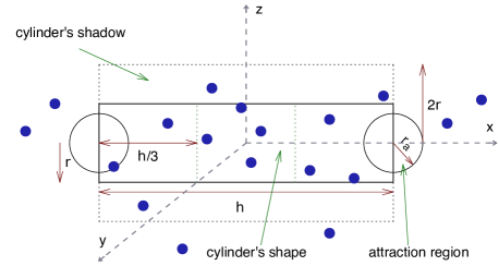
A cylinder is an object characterised by its centre and shape parameters. The shape parameters of a cylinder are the radius , the length , and the orientation vector . The radius is considered fixed. The length varies uniformly within the interval that will be specified later in this paper. The orientation vector parameters are uniformly distributed on , such that
| (2) |
Hence, the mark of our process is given by and its attached uniform distribution . We denote the cylinder by .
Two extremity rigid points (end points) are attached to each cylinder . Around each of these points a sphere of the radius is centred. These two spheres form an attraction region that are used to define connectivity and alignment rules for cylinders (see Sect. 3.4). We illustrate the basic cylinder in Fig. 1, where it is centred at the coordinate origin and its symmetry axis is parallel to the -axis. The coordinates of the end points are
| (3) |
and the orientation vector is .
Let be a configuration of cylinders, where denotes the mark. The unit intensity independently marked Poisson process constructs a configuration of cylinders as follows. First, the number of cylinders is chosen according to a Poisson law of parameter . Then the lengths and the orientation vectors are chosen independently following . Such a configuration has only very few connected and aligned cylinders. This effect is just a chance product. In order to obtain random configurations made of connected and aligned cylinders, a model defined by a probability density is needed. Such a probability density is specified with respect to the reference Poisson process and it can be written
| (4) |
where is the normalising constant, is the vector of the model parameters, and is the energy function of the system (its equivalent in physics is the total Gibbs energy of a system).
We assumed above that locally, galaxies may be grouped together inside a rather small cylinder, and such small cylinders may combine to form a filament if neighbouring cylinders are aligned in similar directions.
Following these two ideas the energy function in (4) can be specified as:
| (5) |
where is the data energy (see Sect. 3.3) and is the interaction energy (see Sect. 3.4) associated with the first and second assumptions above, respectively. In fact, the data energy is related to the position of the cylinders in the galaxy field, whereas the interaction energy is related to the alignment and connection of the cylinders constructing the filamentary pattern.
Being in the possession of the model, the parameters have to be chosen. Here, the Bayesian framework is adopted and the parameters are described by a prior law (Stoica et al., 2007a; Stoica et al., 2007b, 2010). This allows us to write the joint estimator of the filamentary pattern and the parameters as
| (6) | |||||
where is the prior law for the model parameters and is the model parameters space.
The Bayesian framework was preferred, since we believe, that for the problem at hand, it is much more natural to give a characterisation of the parameters by a probabilistic law, instead of a fixed value. Nevertheless, even in this case, some tuning of the model based on trial and error, is needed. The solution we obtain is not unique. In practise, the shape of the prior law may influence the solution, making the result to look more random compared with a result obtained for fixed values of parameters. Therefore, we have derived tools that are able to average the obtained solution and to state that the obtained results are really due to the data, and not to a random effect of the presented methodology (Stoica et al., 2007a; Stoica et al., 2007b, 2010). Full details concerning the set-up of the method and the analysis of the results obtained are given later in this paper.
The paper continues with the presentation of the energy terms, the simulation technique, and an optimisation algorithm.
3.3 Data energy
The data energy term is related to the local definition of a galactic filament. This is still an important open problem. Here, we consider that locally, the galaxies positions form a filament, if they are situated inside a rather small cylinder, while fulfilling simultaneously several criteria. The first one is that the galaxies positions should be spread more or less uniformly a long the main symmetry axis of the cylinder. The second one is that inside a cylinder there should be more galaxies than outside of it, that is inside the close-by neighbourhood of the cylinder. And finally, in order to avoid some clustering effect, the galaxies forming the filaments should be encouraged to get aligned as much as possible along the main symmetry axis of the cylinder.
Under these circumstances, the data energy of a configuration of cylinders is defined as the sum of the energy contributions corresponding to each cylinder:
| (7) |
where is the potential function associated with the cylinder . This potential takes into account the previously mentioned criteria and it depends on (the field of galaxies) and the model parameters given by .
In order to give a mathematical description of these requirements, an extra cylinder is attached to each cylinder , with exactly the same parameters as , except for the radius which equals . Let be the shadow of obtained by the subtraction of the initial cylinder from the bigger cylinder. The cylinder and its shadow are shown in Fig. 1. Then, we divide each cylinder into three equal volumes along its main symmetry axis, and denote by , , and their corresponding shapes.
Let us assume that locally the number of galaxies inside and around a cylinder, follows a Poisson distribution.
The first criteria requires the “local uniform spread” of the galaxies along the main symmetry axis of the cylinder. Under the Poissonian assumption, let be the intensity parameters of the corresponding distributions for the shape regions . If the underlying Poissonian process is stationary, “local uniform spread” requires all the to be equal. However, filaments are lumpy by nature – e.g., the filaments in Pimbblet et al. (2004) and the well-known Perseus Chain (Jõeveer & Einasto, 1978). To take this into account, we relax the uniformity assumption by requiring to be smaller than chosen threshold.
For any two regions and with , a statistical test can be done to compare and (Przyborowski & Wilenski, 1940; Kirshnamoorty & Thomson, 2004). The test is
| (8) |
for all pairs of indices , where is a given threshold value.
Now, for a given pair , the observed number of galaxies in and is and , respectively. Then, the -value for this test is computed using a binomial law of parameters and as follows
| (9) | |||||
Six such tests are necessary to verify the “local uniform spread” condition. The obtained score is
| (10) |
Notice, that this global test is equivalent with verifying with . Hence, it guarantees a minimum density for the galaxies inside a cylinder cell.
The second criteria demands for “locally high density” of galaxies inside of a cylinder comparing to the density of galaxies in the close-by neighbourhood of the cylinder. Under the Poissonian assumption, the test is
| (11) |
with a given threshold value. It is important to notice that the volumes ratio of and plays an important role in choosing the appropriate value of . For instance, if this tests if the two processes have the same intensity, if this tests if the intensity inside the cylinder is three times higher than inside its shadow.
If the observed number of galaxies inside and is and , respectively, the -value of the test is computed using a binomial distribution of parameters and
To take into account both tests simultaneously, the following score is defined
| (13) |
The previous tests are based on counts of points in some pre-defined regions. In order to take into account the spatial distribution of galaxies in a cylinder we define the cylinder concentration as
| (14) |
with the number of galaxies covered by the cylinder, the distance from the th galaxy inside the cylinder to its main symmetry axis, and is the cylinder radius. The weight is chosen to eliminate some pathological cases with too few points covered by a cylinder (there must be at least three galaxies inside a cylinder). Clearly, the concentration has a minimum when the symmetry axis of the cylinder coincides with the least mean square line passing through the cloud of points, given by the galaxy positions inside the cylinder.
It is important to notice that the use of this term may induce a local Gaussian assumption. This may be considered contradictory to the Poisson hypothesis previously used. Nevertheless, the use of these two strategies is complementary: the first two requirements impose conditions on the number of galaxies inside a cylinder, while the third one imposes conditions on the spatial distribution of these galaxies. The term given by (14) is also a very good indicator of a locally high density and a better estimator for the filament axis.
The potential function of the cylinder is built using the previous statistical tests and criteria. Let us assume that for the cylinder , the -value is computed as previously, and let be the cylinder concentration. We want to be maximum for the “best” location of the cylinder in the galaxy field. This allows the definition of the potential function as
| (15) |
with the number of galaxies covered by the cylinder and a given threshold value. Here, the formula (14) suggests . The parameter is required to make the two terms comparable: this allows to use these two strategies safely together.
The data term model (17) is a super-position of inhomogeneous Poisson point processes with respect to the reference measure. Since the number of galaxies is finite and since the observed window has a limited volume, the term is always finite. Therefore, the data term model is locally stable, hence it designs a well defined model that has an integrable probability density.
One more point has to be retained concerning the data term. The use of -values for constructing a potential function is different of the use of the values for “purely” statistical tests. In this last situation Bonferroni or Šidák corrections are required.
3.4 Interaction energy
The interaction energy is related to the relative position of the cylinders forming the network and its expression is as follows
| (18) |
where is the number of repulsive cylinder pairs and is the number of cylinders connected to the network through extremity points. The variables and are the potentials associated with these configurations, respectively.
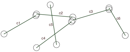
Two cylinders are considered repulsive, if they are rejecting each other and if they are not orthogonal. We say that two cylinders and reject each other if their centres are closer than the minimum allowed distance between cylinders, . Two cylinders are considered to be orthogonal if , where is the scalar product of the two orientation vectors and is a predefined parameter. So, a certain range of mutual angles is allowed for cylinders considered to be orthogonal.
Two cylinders are connected if they attract each other, do not reject each other, and are well aligned. Two cylinders attract each other if the distance between the cylinder end points is smaller than the interaction radius (see Fig. 1). Two cylinders are well aligned if , where is a predefined parameter.
To illustrate these definitions, we show an example configuration of cylinders (in two dimensions) in Fig. 2. Altogether, the configuration at Fig. 2 adds to the interaction energy contributions from three single-connected cylinders (, , ), one doubly-connected cylinder (), two free cylinders (, ), and one repulsive cylinder pair ().
The complete model (4) that includes the definition of the data energy and of the interaction energy is well defined for parameters , , and . The definition of the interactions and the parameter ranges chosen ensure that the complete model is locally stable (van Lieshout, 2000; Møller & Waagepetersen, 2004; Stoica et al., 2005a). This property ensures that we can safely use this model without expecting any dangers (integrability, convergence, numerical stability, etc). The values of the interaction parameters (, ) and of the data parameter have to be fixed taking into account the weight of each energy component and also the underlying galaxy field. If the interaction energy parameters are too strong, then the filamentary network may appear in location where the galaxies form no filaments. If the data energy parameters are too strong, then the filamentary pattern will be well located but not really forming a filamentary network. This is a normal compromise to be found such as in solution regularisation or Bayesian analysis. The Sect. 4.1 shows how these parameters were set.
3.5 Simulation of the model and optimisation algorithm
Several Markov chains Monte Carlo (MCMC) techniques are available to simulate marked point processes: spatial birth-and-death processes, Metropolis-Hastings algorithms, reversible jump dynamics or more recent exact simulation techniques (Geyer & Møller, 1994; Green, 1995; Geyer, 1999; Kendall & Møller, 2000; van Lieshout, 2000; van Lieshout & Stoica, 2006).
In this paper, we need to sample from the joint probability density law . This is done by using an iterative MCMC algorithm. An iteration of the algorithm consists of two steps. First, a value for the parameter is chosen with respect to . Then, conditionally on , a cylinder pattern is sampled from using a Metropolis-Hastings algorithm (Geyer & Møller, 1994; Geyer, 1999).
The Metropolis-Hastings (MH) algorithm we used is built using three types of moves (van Lieshout & Stoica, 2003; Stoica et al., 2005a; Stoica et al., 2007b, 2010).
-
•
Birth: with a probability a new cylinder , sampled from the birth rate , is proposed to be added to the present configuration . The new configuration is accepted with the probability
(19) -
•
Death: with a probability a cylinder from the current configuration is proposed to be eliminated according to the death proposal . The role of this move is to ensure the detailed balance of the simulated Markov chain and its convergence towards the equilibrium distribution. The probability of accepting the new configuration is computed reversing the ratio (19).
-
•
Change: with a probability we randomly choose a cylinder in the configuration and propose to slightly change its parameters using uniform proposals. For the selected element, we may change its location within the vicinity of its centre and change its orientation within a small angle tolerance with respect its initial orientation. The new element obtained is . This move improves the mixing properties of the sampling algorithm. The new configuration is accepted with the probability
(20)
Some practical details concerning the MH dynamics implementation are given below. For a complete description we recommend van Lieshout & Stoica (2003) and Stoica et al. (2005a).
The uniform choices and are commonly adopted for their simplicity and because they guarantee the necessary convergence properties of the simulated Markov chain, such as irreducibility, Harris recurrence, and geometric ergodicity. For the probabilities , , and , all the convergence properties are preserved as long as . Here, is the Lebesgue measure (volume) and is the number of cylinders in the configuration.
Nevertheless, when the model to simulate exhibits complicated interactions, such an update mechanism built of uniform birth and death proposals may be very slow in practice. Here the strategy proposed by van Lieshout & Stoica (2003) and Stoica et al. (2005a) is adopted. This strategy uses adapted moves that help the model. In our case, the new cylinder can be added uniformly in (the observed volume) or can be randomly connected with the rest of the network. This mechanism helps to build a connected network and it can be implemented using a non-uniform mixture for the birth proposal
| (21) |
with ( is the probability to add a connected cylinder) and is a probability density proposing attracting and well aligned (e.g. connected) cylinders. The expression of is given by
| (22) |
where is the set of cylinders in the configuration which have at least one end point able to create connections, and is the number of such cylinders in the configuration. Note that neglecting the edge effects, is the number of 0- and 1-connected cylinders in configuration. After choosing uniformly an object from the set , a new object is proposed to be added using the density
| (23) |
where is the region built from the union of attraction balls of which are not containing the end of any other attracting cylinder in the configuration , is the volume of those attraction balls, and is the indicator function that selects the cylinders the new cylinder may be connected with. Here, one end point of the proposed connected cylinder is uniformly distributed in and the orientation is uniformly chosen to satisfy the well-aligned criterion . Clearly, the summation in Eq. (22) is effectively over the cylinders the new cylinder can be connected with.
This birth rate leads the model to propose configurations with connected objects much more often than using the simple uniform proposal. In practice, it is also reasonable to sample only in the regions where the data potential is defined: . Hence, the Lebesgue measure in this case can be calculated as
| (24) |
In order to perform the maximisation of , the previously described sampling mechanism is integrated into a simulated annealing algorithm. The simulated annealing is a global optimisation method. It iteratively samples from , while goes slowly to zero. Stoica et al. (2005a) proved the convergence of a simulated annealing algorithm based on a Metropolis-Hastings dynamics for marked point processes, if a logarithmic cooling schedule is used. According to this result, the temperature is lowered as
| (25) |
where is the initial temperature.
4 Extracting and defining the filaments
In this section we describe how we set up the experiment and extract the filaments. Our aim is to use the result obtained using marked point processes to compile a filament catalogue. Every filament in this catalogue is represented as a spine: a set of points that define the axis of the filament.
| Param. | Description | Value |
| cylinder radius | 0.5 | |
| cylinder length | ||
| locally high density | 1.0 | |
| locally uniform spread | 4.0 | |
| minimum number of galaxies | 3 | |
| hypothesis test coefficient | ||
| attraction radius | 0.5 | |
| orthogonal cylinders | 0.30 | |
| parallel cylinders | 0.15 | |
| repulsive cylinders | 0 | |
| 0-connected cylinders | ||
| 1-connection cylinders | ||
| 2-connection cylinders | ||
| birth/death/change probabilities | 0.5/0.2/0.3 | |
| connected birth probability | 0.8 | |
| max shift for change move | 0.2 | |
| min cosine for orientation change | 0.95 | |
| initial temperature | 5.0 | |
| steps between temperature changes | 100 000 | |
| number of cycles | 200 000 | |
| number of simulations | 50 | |
| limiting visit map value for filaments | 0.05 | |
| limiting orientation strength | 0.75 | |
| limiting angle for filaments | 0.95 | |
| limiting curvature for filaments | 1.0 |
4.1 Experimental setup
As described above, we use the data set drawn from the SDSS contiguous area. The sample region is the observed volume in space.
In order to choose the values for the dimensions of the cylinder, we use the physical dimensions of galaxy filaments that have been observed in more detail (Pimbblet et al., 2004); we used the same values also in our previous papers (Stoica et al., 2007b, 2010): a radius . The same scale has been also used by Smith et al. (2012) and Tempel et al. (2013) showed that filaments of this size may influence galaxy evolution, so this seems to be the most interesting scale for galaxy filaments. Naturally, the nature of filaments is hierarchical (Shen et al., 2006; van de Weygaert & Bond, 2008a, b; Aragón-Calvo & Szalay, 2013) and the chosen scale of filaments can be arbitrary. In the present paper, we aim to detect filaments that have the strongest impact on galaxy evolution: for that the scale should be relatively small. Taking into account the data resolution in the SDSS, the scale is the minimal one we can choose. The length of a cylinder is chosen to be –, which is the shortest possible (the ratio of the cylinders length to its diameter is 3:1 to 5:1). The length in this range is considered to be free to more effectively sample the low number density regions.
We choose the attraction radius , which ensures that the end points of connected cylinders are not too far apart. For the cosines of the maximum curvature angles we choose and . This allows for a maximum of between the direction angles of connected cylinders and considers the cylinders to be orthogonal, if the angle between their directions is larger than .
The model parameters influence the detection results. If they are too low, no filaments will be detected. If they are too high, the detected filaments will be too wide and/or sparse, and precision will be lost. Still, the precision can be increased and the influence of model parameters can be minimised, when sets of simulations and visit maps are used (see Sect. 4.2): in a certain manner, it will average the detection results. In this work, the model parameters were chosen based on a previous knowledge and after a visual inspection of the detected filamentary pattern.
Fixing the data and interaction energy parameters require an “initial guess” of the size of the solution. This guess does not need to be precise. The stochastic algorithmic “machinery” will do the job, due to its mathematical theoretical properties. Nevertheless, from a practical point of view, if the range of parameters allows only very few cylinders in the configuration, then the detection may be incomplete. On the other hand, if too many cylinders are allowed, then the detection may contain a lot of false alarms. Attention should be also paid when the measure units are fixed. A transformation of the measure units induces a transformation of the model parameters so that the same probabilities are assigned to the same configurations of objects. Still, a direct relation between the change of the measure units and the model parameters is not easy to be derived, because of the non-linear character of the model. Under these circumstances, the strategy we have adopted is the following. It is generally accepted that the filaments occupy roughly 10% of the observed volume (Forero-Romero et al., 2009; Jasche et al., 2010; Aragón-Calvo et al., 2010b). In the actual observed volume of the SDSS the observed filamentary network is made of (roughly speaking, and with respect to the chosen unit measure), about cylinders. This gives a coarse cylinder density of about of cylinders per unit of volume. Hence, a very intuitive way of fixing the range of parameters is to equalise this density with the probability density given by the model of having a cylinder in an observed location. This probability density is naturally approximated by the conditional intensity of the model. Hence, we get
| (26) |
or
| (27) |
where is the new cylinder to be added to the configuration .
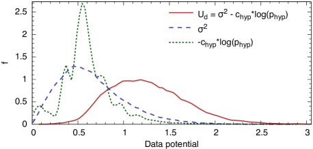
The definition of the data energy needs some predefined parameters. To test for the “locally high density”, we fix : the assumed number density in a filament should be at least three times larger than in its outer layers. For the “locally uniform spread” we set , this allows some lumpiness along the filament and at the same time penalises filaments that cross large clusters. The minimum number of galaxies inside a cylinder is set to be . To assure balance between the concentration and hypothesis testing terms, the constants in front of the hypothesis testing term is chosen to be . The value is chosen uniformly within the given interval. The distribution of the cylinder data potentials after the simulation are shown in Fig. 3, together with the distributions of the hypothesis testing term and the cylinder concentration term: we see that for given data and chosen parameters, these two terms are comparable and the overall data potential is reasonable.
For interaction energy, the potentials (, ) are chosen from an uniform prior density . We have opted for this choice since no information concerning the relative strength is available (Stoica et al., 2007a; Stoica et al., 2007b, 2010). Still, the general guidelines for fixing the prior parameters are that 2-connected cylinders are generally encouraged, while 1-connected cylinders are slightly penalised and 0-connected cylinders are strongly penalised. This choice encourages the cylinders to group in filaments in those regions where the data energy is good enough. Hence, the prior domain was set to , , and . The repulsion parameter , so configurations of repulsing cylinders are forbidden. The prior domain for was chosen based on the distribution of data energies (see Fig. 3): the chosen domain have to be in balance (in the same range) as data potentials for cylinders.
In Table 1 the parameters of the Metropolis-Hastings algorithm and the simulated annealing algorithm are also given. For the change move, the maximum shift for the cylinder centre is and the minimal cosine between the old and new direction angles is . We use a uniform prior for cylinder shift in a spherical volume with radius : orientations are taken uniformly on a unit sphere.
4.2 Extracting the filamentary pattern spine
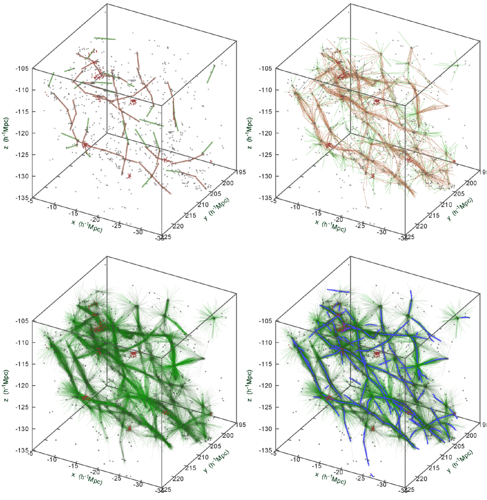
The solution provided by our model is stochastic. Therefore some variation in the detected patterns is expected for different runs of the method. In Fig. 4 (upper left panel) a single MCMC simulation is showed, while indicating the different types of cylinders: isolated (grey), single-connected (green), and double-connected (red). The Fig. 4 (upper right panel) presents the superposition of independent simulations. It can be seen, that the main features of the filamentary pattern are detected by most of the simulations, while differences that appear are due to the random effects of the method.
In order to have a more precise measure of these differences, a brief statistical exploratory analysis was done. To do this the sufficient statistics of the model (the number of 0,1,2-connected cylinders) were analysed. In one simulation, the simulated annealing algorithm run during steps or moves. One step consists of one iteration of the transition kernel of the MH dynamics, that is an accepted or rejected birth or death or change proposal. The temperature was lowered every iterations (one cycle): this number of moves was considered sufficiently high in order to obtain almost un-correlated samples. Finally, we get samples per simulation. In all, we have considered independent simulations.
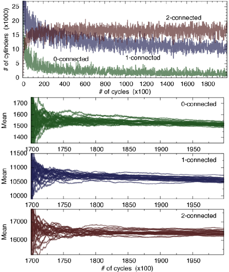
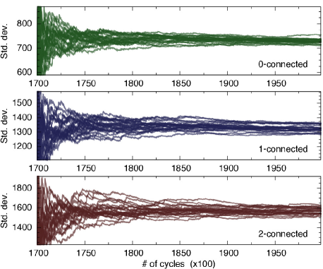
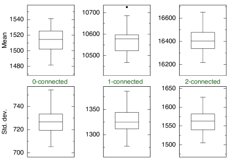
The results of the exploratory analysis are shown in Figs. 5 and 6. Figure 5 (upper panel) shows the number of cylinders in configuration as a function of cycles. We see that initially the number of 2-connected cylinders increases but it remains roughly constant after a certain time. The number of 0- and 1-connected cylinders decreases: this decrease is expected since simulated annealing penalises these cylinders more over time. Eventually, these numbers also approach a constant value. The three lower panels in Fig. 5 show the cumulated means for the final part of the simulations: superposition of 50 simulations are shown. From this figure we see that the number of 0,1,2-connected cylinders tend to have similar statistical values in every simulation. The cumulative standard deviations are shown in Fig. 6. The box-plots of the mean and standard deviation distributions obtained from the final realisation of 50 independent simulations are shown in Fig. 7. The standard deviation is much larger than the variation in mean numbers of cylinders, showing that all the 50 simulations are statistically equivalent.
These numerical results are coherent with the detection obtained in Fig. 4. The robust part of the network is given by the 2-connected cylinders. The part of the network made of 0- and 1-connected cylinders may be considered at a quick look as “noisy”. Still, the question what part of this “noisy” part is relevant for the filamentary network, is of real interest. Our manner of answering it was to leave the model parameters rather free, since we do not know exactly how the objects we are looking for look like. Averaging several simulation results and spine detection should eliminate the “noisy” part while keeping the important short filaments.
There is another point to be outlined. Our plots show that simulated annealing does not reach convergence yet (in theory, it converges at infinity). This is due to the real computational time needed for getting the results: with modern computers, one simulation takes approximately 1000 CPU-hours in a single CPU. There was a compromise to be done here: choosing an appropriate cooling schedule and stopping the algorithm after a while, or choosing a fast cooling schedule and stating that the algorithm “converged”. We have chosen the first approach. The convergence of the MCMC simulation methods is still an open research problem. For the reader interested to get a deeper insight of this very interesting problem we recommend as a starting point Robert & Casella (2004).
The main advantage of using such a stochastic approach consists in the ability of the model to give a simultaneous morphological and statistical characterisation of the pattern. This allows the comparison of several filamentary networks and this idea was used in a previous study to compare mock catalogues and observed data (Stoica et al., 2010). Nevertheless, it is legitimate to wish to have a smooth map of these filaments. A solution to this problem is, under the hypothesis of the model, to estimate the probability that a point belongs to the filamentary network and to look at those regions where these values are higher than a given threshold (Stoica et al., 2007a; Stoica et al., 2007b, 2010). Several realisations should be used to estimate this quantity and the filamentary network is smoothed. In our previous work, these quantities are called visit maps, and this name is kept in the following, due to its suggestivity. In mathematics, these quantities are known as level sets and the convergence of these type of estimators was studied in Heinrich, Stoica & Tran (2012). The visit map estimated from a number of realisation is shown in Fig. 4 (lower left panel).
Another very important aim of our work is to link the richness of our approach with the very efficient existing deterministic methods for filaments finding. Therefore, in the following a method for filamentary pattern spine detection is proposed. Figure 4 (lower right panel) shows the result of the introduced method. The main difference with the existing methods is that the spine detector we build uses the information provided by our stochastic approach. This information consists of different quantities that can be estimated locally using our model. These quantities estimate different probability and visit maps and also statistics related to the orientation field induced by the filamentary network.
The spine detection we propose is based on two main ideas. The first idea is that filament spines are situated at the highest density regions outlined by the filament probability maps. Next, in these regions of high probability for the filamentary network, the spines have an orientation that is aligned with the direction given by the orientation field of the filamentary network. On the contrary, in cross sections of filaments, the filament detection probability can be high, but the orientation field is not clearly defined. The filament spine detection method is described below in detail.
First, we re-call the visit map estimator for a given point
| (28) |
where are cylinder configurations and is the indicator function testing whether the point belongs to any of the cylinders in the configuration . By this definition, the visit map is defined to be in the range .
The density map of filaments is defined as a weighted visit map (level set). For a given point it is defined as
| (29) |
where the first summation is over realisations and the second summation is over cylinders in that given configuration . The potential function for a cylinder is defined by Eq. (15). The indicator function acts as a cylindrical kernel and selects the points that the cylinder covers. Note that a point can be covered by a several cylinders in one configuration, but effectively all configuration have equal weights. We weight the visit map to suppress weak intersecting filaments (to reduce the noise) and to encourage stronger filaments.
The orientation field for a point and for a orientation is defined as
| (30) |
where denotes the scalar product between the orientation vector and the cylinder orientation . Using this definition, . Using the orientation field, we also define density field for orientation strengths: the maximum of the orientation field depending on at a given location is ,
| (31) |
This quantity is a weighted estimator of the expectation of the scalar product between the orientation at the location . If the cylinder orientation is uniform on the unit sphere, then the absolute values of the scalar product is a uniform random variable between and . Hence the value of under the uniform assumption should be close to . If all the cylinders are aligned with respect to then the value of should be close to . If we are interested in the situation that the majority of cylinders are aligned to , then we may test with a pre-defined threshold value rather close to . For our purposes we set , since this value may suggest a half way distance between the uniform and the completely aligned case.
The corresponding orientation of the maximum value at location is and it is defined as
| (32) |
For computing the previous estimators the last extracted realisation from a single run of the algorithm were kept: we extracted the realisations after 1000 cycles. In total we have used independent runs of the algorithm. This gives in all cylinder configurations to be used for computing the previous defined quantities.
At a first look, the previous quantities can be computed locally, hence there is no need for keeping track of the cylinder configurations. In our case we need to calculate the visit map (and orientation map with orientations) in a grid with grid-step smaller than 0.1 Mpc to accurately determine the spine of the filaments. Due to the limitations of the computer memory, it cannot be computed globally for the entire simulation box. In order to calculate the visit map and orientation map with sufficiently fine grid, they have to be computed locally. For that purposes, we store the cylinder configurations from every simulations and compute the visit maps and orientation maps locally as defined above. The advantage of this approach is that all required quantities can be computed for every space and orientation in the sample volume and we are free of gridding. The chosen 1600 cylinder configuration is large enough for visit map and orientation map estimation and at the same time it requires reasonable amount of computational resources.
Using previous definitions, for every point we have three values: the filament density , the orientation strength , and the filament orientation in that location . To extract a single filament using these three quantities, we do the following.
-
1.
We start at a point of the highest density that is not yet masked out (we will discuss masking later). We designate this point as . The initial density map is calculated on a 0.5 Mpc grid, which is sufficiently fine (compared with cylinder size) for global maxima. After maximum is found, the density map is calculated locally on a 0.01 Mpc grid. Initially, all the regions where are masked out: e.g. we are searching for the filaments in the regions that have been covered at least in 5% of the realisations. We remind that all the detected structures are filaments by definition, and this is only the detection probability that depends on the model parameters.
-
2.
If the orientation at that point is defined, we start extracting a filament. We say that the orientation is defined if . Otherwise, we mask out the region around this point and continue with the step (i). The size of the masked region is taken as .
-
3.
We look from the point to both sides along .
-
4.
To extract the filament, we move from the point in the direction by . The step size is arbitrary, but a smaller step size gives smoother filaments. The step size is good enough ( is the cylinder radius). We designate the new point as .
-
5.
We calculate the density map that is perpendicular to the direction . The density map is two-dimensional and from that map we find the maximum that is closest to the point : the location of this maximum is marked as .
-
6.
If the orientation is not defined at , we stop the filament extracting algorithm and continue with the step (x).
-
7.
If the orientation is defined () we go forward by and find a new point as previously explained. This point is needed to perform two additional checks.
-
8.
Firstly, to avoid breaks in the filament, we calculate the curvature of the filament at the point using this point and its neighbours. The curvature , where is the radius of the sphere that these three points touch. We use the limiting value to stop the filament finding algorithm.
-
9.
Secondly, we require that the orientation at the point and at the neighbouring points is roughly the same:
(33) If the tests are not satisfied, we stop the filament finding algorithm. Otherwise, we move in the direction by and continue with the step (v).
-
10.
If all the filament points from both sides of have been found, we mask out the region that this filament covers. The radius of the masked out region is taken (twice the filament radius). We save the extracted points as a single filament.
-
11.
We return to the point (i) until all the volume is masked out.
Basically, this algorithm walks along the mountain chain in the filament density map and tests if the orientation is defined and the orientation is the same as the walking direction. There are only four parameters that define the filaments: defines the limiting visit map density and the strength of a filament, defines the orientation and estimates the strength of orientation for a filament, defines the limiting curvature, and defines the angle between the filament and the orientation field. All these criteria are unimportant for strong filaments, but they influence the regions where filaments intersect or the regions where filaments are poorly defined.
5 Results and discussion
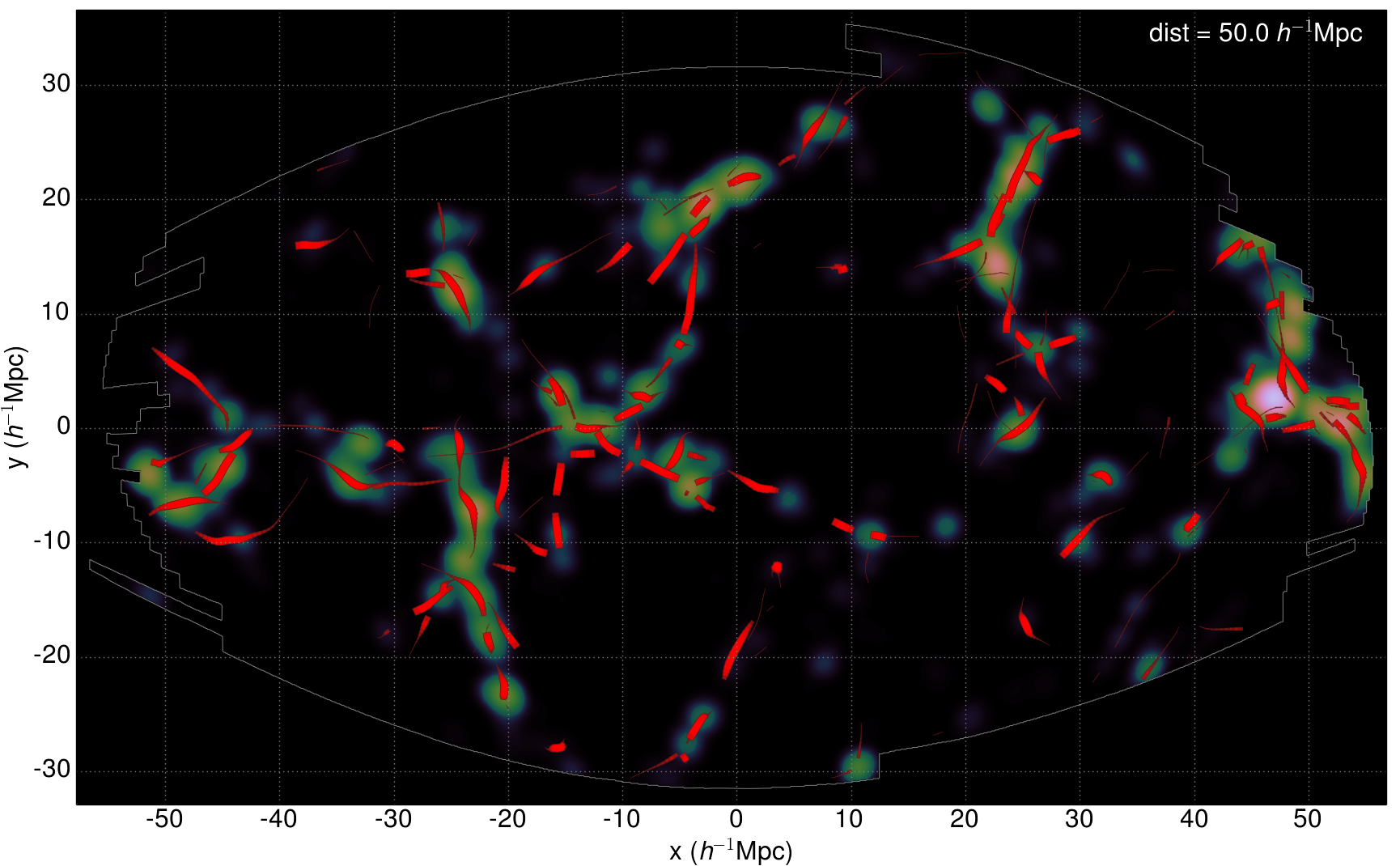
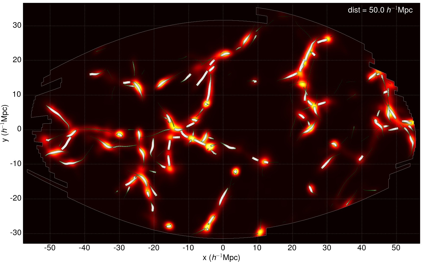
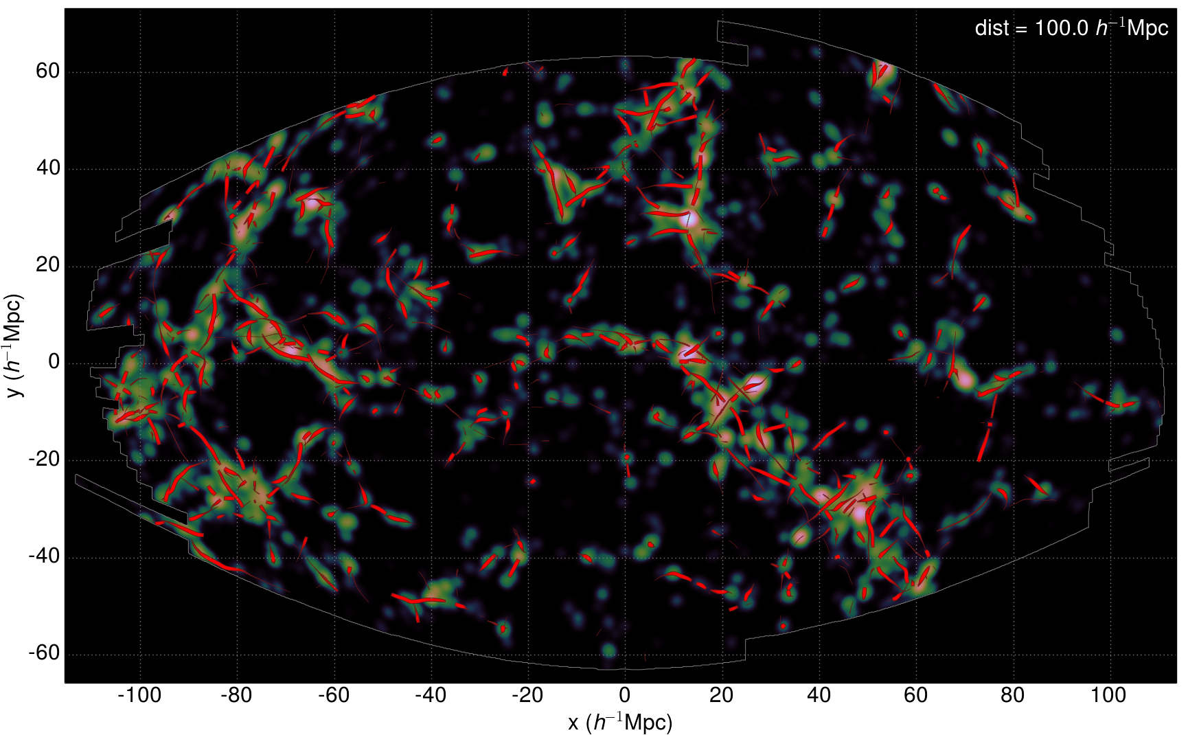
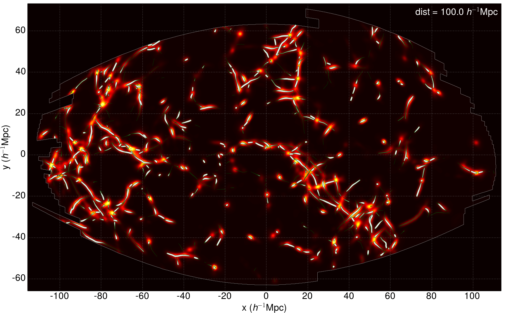
Figure 8 illustrates the detected filaments and their axes. In left panel are shown the luminosity density field smoothed with 1 Mpc -spline kernel. Right panel shows the corresponding visit map () for detected filaments. Extracted filament spines are shown with lines. Qualitatively, the filament axes plotted in these figures appear to closely trace the underlying large-scale filaments. This is not surprising because, by definition, our filament finder is based on cylindrical shapes and the filament detection probability field should trace the filamentary structures. Tempel et al. (2014) used the Bisous process to detect the filaments from dark matter simulations and showed that the detected filaments are very well aligned with the underlying velocity field. This shows that the detected filaments are also dynamical structures.
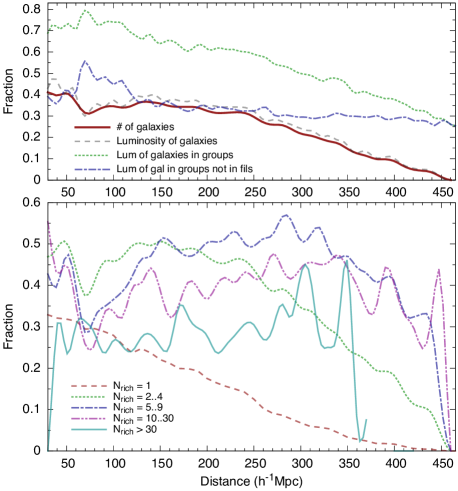
The upper panel in Fig. 9 shows the fraction of galaxies in filaments as a function of distance: the red solid line shows the number of galaxies and the grey dashed line shows the fraction of luminosity in filaments. We note that there is slightly more luminosity in filaments than the number fraction predicts – meaning that in filaments the luminosity density of galaxies is higher than in average. The green dotted line in the upper panel of Fig. 9 shows the fraction of luminosity that is in groups (we use the groups as defined in Tempel et al., 2012). Since we use a flux-limited sample, the number density of groups (and their luminosity) is higher for nearby regions. The blue dot-dashed line shows the fraction of luminosity in groups that are not in filaments. We see that this fraction is almost constant. The lower panel in Fig. 9 gives an explanation for that. Most of the galaxies that are in filaments are also in small groups and since filaments have a chain-like inner structure, the nearby filaments are made of smaller groups that are aligned. Further away, the number density of smaller groups is lower and the filament detection probability is also lower (the red solid line in the upper panel). The lower panel in Fig. 9 also shows that isolated galaxies are preferentially not located in filaments and also the galaxies in large clusters are mostly not in filaments: only galaxies in the outskirts of large clusters are in filaments.
All this implies that filaments are far from being smooth uniform structures. Visual inspection of the density field and the spines of filaments (Fig. 8) shows that filaments are populated by small galaxy groups and large clusters are in intersection of those filaments, as already shown in Bond et al. (1996). The same impression is quantitatively confirmed in Fig. 9.
The fraction of galaxies (or luminosity) in filaments gives us roughly the mass filling fraction of filaments. Up to distance , the fraction is 35–40%, which is in very good agreement with -body simulations (Forero-Romero et al., 2009; Aragón-Calvo et al., 2010b; Hoffman et al., 2012). Using the SDSS data, the same filament mass filling fraction has been measured by Jasche et al. (2010). We note that after , the number of detected structures decreases. Smith et al. (2012) search structures in the SDSS in the same scale as we, and their number of detected structures follows the same behaviour with distance. This is logically expected, since the number density of objects (that decreases with distance in flux-limited survey) is strictly related to the number of detected structures.
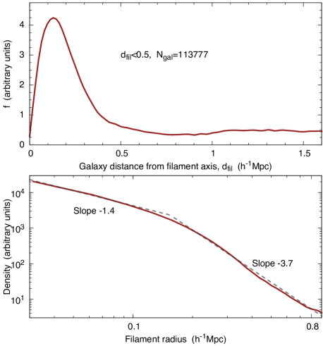
Although filaments have been studied extensively in general, there are only few studies addressing their radial density profile (Colberg et al., 2005; Dolag et al., 2006; Aragón-Calvo et al., 2010b). However, in these papers, larger filaments are considered, so a strict comparison is not possible. Figure 10 shows the filament radial profile in the current study: the upper panel shows the distribution of the number of galaxies per radius, the lower panel shows the number density profile for filaments. We see that most of the galaxies in filaments are closer than Mpc to the filament axis. This is because our defined filament radius is Mpc. We also see that there is a break in the density profile around Mpc. Using weak lensing, Jauzac et al. (2012) studied a single filament that connects two clusters and they also see the break in the density profile roughly at the same distance. Direct comparison with other studies is possible, once we extract thicker filaments: this is planned for future work.
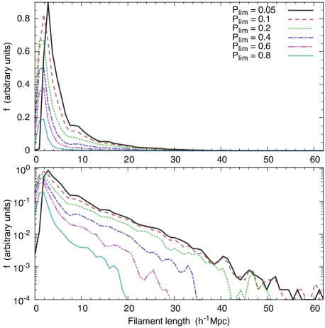
Another interesting quantity is the filament length distribution. Figure 11 shows the filament length distribution in the linear (upper panel) and logarithmic (lower panel) scale. The distribution is shown for different minimum detection probability values (). The black solid line shows the filaments as given in our catalogue. Increasing the limiting detection probability, the filaments start to fragment and small (weak) filaments disappear. We see that increasing the detection probability up to 0.2 practically does not change the long-end of the distribution. The longest filaments are strong and dominant filaments. We emphasise that the value of the detection probability is model dependent and it does not reflect the probability of the filamentary structure (all detected structures in our model are filaments based on the definition).
The filament length distribution has been also studied in Bond et al. (2010b) using -body simulations. Compared with our length distribution, the longest filaments are roughly the same, but we have more short filaments. This is probably because the spatial distribution of observed galaxies is sparse and in many cases we only found a piece of a filament.
The maximum length of our filaments is . This is in very good agreement with other measured values (Bharadwaj, Bhavsar & Sheth, 2004; Bond, Strauss & Cen, 2010b; Pandey et al., 2011).
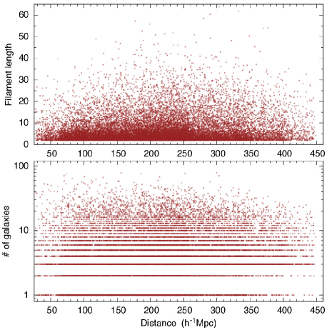
Figure 12 shows the filament lengths and the number of galaxies in filaments as a function of distance. We note that both distributions are quite uniform. There is lack of long filaments in the nearby region because its volume is small. Further away, the longest filaments are missing because the number density of galaxies is too low. However, there exist filaments with lengths up to Mpc further than Mpc. The number of galaxies in filaments (lower panel) decreases with distance because we used a flux-limited sample: the faintest galaxies are missing further away.
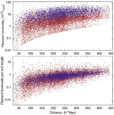
Figure 13 shows the luminosity of a filament (upper panel) and the luminosity per unit length (lower panel) as a function of distance. We notice that the faintest filaments are missing further away, because of the flux-limited survey. However, the upper limit is distance independent and it shows that the brightest filaments nearby and further away are practically the same. We also note that the scatter in the lower panel is quite small, indicating that luminosity per unit length in filaments does not vary much. Blue points in the figure show the longest filaments (at least Mpc long). We see that the longest filaments are also the most luminous filaments, however, their luminosity per unit length lies within the average. This indicates that short and long filaments have on average the same luminosity density.
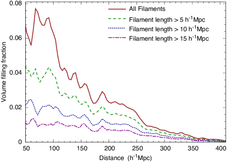
One important quantity that describes filaments is their volume filling factor. Figure 14 shows the volume filling factor as a function of distance. Since the number density of galaxies decreases with distance, the volume filling factor also decreases. The filament volume is calculated around the detected spines, using the filament radius ; in the nearby region, the filling factor is and it decreases with distance (due to the flux-limited survey). From -body simulations, the volume filling factor has been measured by Forero-Romero et al. (2009) and Aragón-Calvo et al. (2010b). In these papers, the volume filling factor depends on the used threshold, but it is in order of 10%, which is in good agreement with our results. Based on the SDSS data, the filaments have been extracted by Jasche et al. (2010). They use a novel Bayesian sampling algorithm, which permits precise recovery of poorly sampled objects in a non-linear density field. Based on their analysis, the filament volume filling factor is 10–20%, which is slightly larger than ours. However, since they use a grid their filaments are thicker than ours and these results cannot be directly compared. On the contrary, Hoffman et al. (2012) showed that the filament volume filling fraction is 4–5% using the velocity shear tensor. This is slightly lower than we found in the current study (considering the fact that we do not detect all structures). Since the mass filling fractions in both studies are comparable, the filaments found in the velocity field are probably located mostly in higher density environments and are somewhat thicker (Tempel et al., 2014).
5.1 Robustness of the filamentary pattern detection
Our method is sensitive to the galaxy density. If a data set contains too few galaxies, no filaments will be detected since the filamentary pattern is not observable. If the data set contains many galaxies, the filamentary network is already defined, hence our method will always work. Indeed, intuitively, there is an optimal range for the galaxy number density so that our model delineates correctly the filaments.
In general, the model parameters depend on the minimum number density. The model parameters of our “machinery” were designed studying the SDSS data set. After several trials and errors, we found the parameter values that give the best results (see Table 1). To reliably determine filaments, two (preferentially three or more) cylinders have to be aligned and connected. With the present model parameters, this leads to the minimum number density (inside a filament) of 6 galaxies within a cylindrical volume of the radius 0.5 and the length 6–10 Mpc.
As the data energy in our model is determined by the ratio of densities in the cylinder and its shadow, it does not depend on the local number density of galaxies (for fixed model parameters, and if the minimum number density condition is satisfied). This allows us to detect physically similar filaments regardless of the environmental density, and our method can recover structures of relatively sparsely sampled objects (filaments in lower density environments).
In a flux-limited survey, the number density of galaxies decreases with distance. For our model, it means that the filament detection probability decreases (we do not detect all filaments further away and/or we only detect parts of the filamentary network), but the reliability of the detected filaments, determined by the visit map value, is largely unaffected, due to the robustness of the model.
As an example, Figure 14 shows the volume filling fraction of filaments as a function of distance. Including all filaments (red line), the sample is not homogeneous. However, it is possible to construct a statistically homogeneous sub-sample of filaments, when the sample is limited by distance and filament length. Figure 14 shows that when using only longer filaments, the volume filling fraction is roughly constant with distance up to 240 Mpc. Further away, the galaxy number density decreases rapidly, and the full filamentary network for the scale used here () is not clearly outlined.
Another important point to be raised is the question whether the optimal choice of the model parameters should depend on the galaxy number density. Stoica et al. (2010) addressed this issue and concluded that simple choices (e.g. increasing the cylinder size) do not produce good results: different cylinder sizes detect different structures. To reduce the incompleteness in filament detection, larger cylinders should be used everywhere to detect the same structures.
How can shot noise affect the filament detection in low number density regions? Like for any other methods, shot noise affects the results. The main advantage of our method is in its probabilistic nature. Individual realisations of the solution may be sensitive to noise. Still, averaging these realisations reduces the noise influence, and allows computation of robust statistical quantities (Stoica et al., 2010). These quantities are the estimates of the sufficient statistics, the level sets (visit maps) and the local detection probability.
It is also possible to think about the reverse formulation of the detection problem. That is, knowing the topological structure of the filamentary pattern, we may wonder what is the density range within the observed volume, that still outlines the given filamentary network. However, the optimal model choice for filament detection, is at the moment an open mathematical and data analysis problem.
6 Conclusions and future work
This paper uses and develops an object point process with interactions (the Bisous process) to trace the filamentary network in the flux-limited SDSS data. This method works directly on the galaxy distribution and does not require any additional smoothing, it only requires fixing the scale of structures. For the current work, we fixed the radius of a filament as , which is close to the scale of galaxy groups/clusters; such filaments should have the largest impact for galaxy formation and evolution.
Our filament finder is probabilistic in the sense that it gives us the filament detection probability field together with the filament orientation field. Using these two fields, we define the spines of the filaments and extract single filaments from the data. We showed that the detected filaments fit well with the visible large-scale structure. The composed catalogue of filaments for the SDSS is made publicly available (see Appendix A).
We showed that the filament mass and volume filling factors are in good agreement with structures found in -body simulations and in previous observational studies. The mass filling fraction of our filaments is 35–40%, and the volume filling fraction is and decreases with distance due to the flux-limited data. Consequently, filaments contain the largest fraction of mass in the Universe and they represent the most salient component of the cosmic web: they form the bridges between all structural features at the group/cluster scale.
Our catalogue of filaments is not the first attempt to extract filaments from SDSS data. Filaments from SDSS have been extracted by Sousbie et al. (2008), Jasche et al. (2010), and Smith et al. (2012). In the following studies, we plan to compare how various filament finders work and how the filaments detected using different methods differ.
In our method we have to define the filament scale (radius). In the current study it is fixed at Mpc. This scale was chosen to find the bridges between galaxy groups and because it was known that this scale affects the galaxy evolution (e.g. Tempel et al., 2013; Tempel & Libeskind, 2013). Since filaments are hierarchical by nature (Aragón-Calvo et al., 2010b; Smith et al., 2012) it is interesting to search for filaments at many scales. The number density of galaxies in the SDSS does not allow to search for smaller filaments. We are preparing our filament finder to search for thicker filaments, and the catalogue and comparison of multi-scale filaments will be our next step. The multi-scale filaments will allow us to better determine the filament scale that affects galaxy evolution.
Figure 9 shows that galaxies in large clusters are not in filaments. This is expected since filaments are the bridges between clusters and large clusters are in intersection of many filaments (Aragón-Calvo et al., 2010b). In our following work, we plan to study how filaments and groups/clusters are connected and how this connection depends on cluster/filament properties.
The Bisous process can also be applied to other structure elements, as clusters, sheets, and voids. This is also one the future directions of our work.
Acknowledgments
We thank our colleagues in the Cosmology Department of Tartu Observatory for useful discussions that helped to clarify many aspects in the paper. We thank the referee for his/her constructive comments and questions.
We acknowledge the support by the Estonian Science Foundation grants 9428, MJD272, PUT246; the Estonian Ministry for Education and Science research project SF0060067s08; the Centre of Excellence of Dark Matter in (Astro)particle Physics and Cosmology; by the Spanish Ministry of Science and Innovation project AYA2010-22111-C03-02, and by the Generalitat Valenciana project of excellence Prometeo 2009/064. E.S. acknowledges a visiting professor grant of the Vicerrectorado de Investigación y Política Científica de la Universitat de València. E.T. and E.S. also thank the hospitality of the Observatori Astronòmic, Universitat de València and Université Lille 1 where part of this work was performed. R.S. thanks the Université Lille 1, the GDR 3477 Géométrie stochastique, the Tartu Observatory and the Valencia Observatory for the financial and scientifical support. This work was carried out in the High Performance Computing Center of University of Tartu. All the figures have been made using the gnuplot plotting utility or matplotlib (Hunter, 2007). This research has made use of NASA’s Astrophysics Data System Bibliographic Services.
Funding for SDSS-III has been provided by the Alfred P. Sloan Foundation, the Participating Institutions, the National Science Foundation, and the U.S. Department of Energy Office of Science. The SDSS-III web site is http://www.sdss3.org/.
SDSS-III is managed by the Astrophysical Research Consortium for the Participating Institutions of the SDSS-III Collaboration including the University of Arizona, the Brazilian Participation Group, Brookhaven National Laboratory, Carnegie Mellon University, University of Florida, the French Participation Group, the German Participation Group, Harvard University, the Instituto de Astrofisica de Canarias, the Michigan State/Notre Dame/JINA Participation Group, Johns Hopkins University, Lawrence Berkeley National Laboratory, Max Planck Institute for Astrophysics, Max Planck Institute for Extraterrestrial Physics, New Mexico State University, New York University, Ohio State University, Pennsylvania State University, University of Portsmouth, Princeton University, the Spanish Participation Group, University of Tokyo, University of Utah, Vanderbilt University, University of Virginia, University of Washington, and Yale University.
References
- Aihara et al. (2011) Aihara H. et al., 2011, ApJS, 193, 29
- Alpaslan et al. (2013) Alpaslan M. et al., 2013, MNRAS, accepted, arXiv:1311.1211
- Aragón-Calvo (2013) Aragón-Calvo M. A., 2013, arXiv:1303.1590
- Aragón-Calvo & Szalay (2013) Aragón-Calvo M. A., Szalay A. S., 2013, MNRAS, 428, 3409
- Aragón-Calvo et al. (2007a) Aragón-Calvo M. A., Jones B. J. T., van de Weygaert R., van der Hulst J. M., 2007a, A&A, 474, 315
- Aragón-Calvo et al. (2007b) Aragón-Calvo M. A., van de Weygaert R., Jones B. J. T., van der Hulst J. M., 2007b, ApJ, 655, L5
- Aragón-Calvo et al. (2010a) Aragón-Calvo M. A., Platen E., van de Weygaert R., Szalay A. S., 2010a, ApJ, 723, 364
- Aragón-Calvo et al. (2010b) Aragón-Calvo M. A., van de Weygaert R., Jones B. J. T., 2010b, MNRAS, 408, 2163
- Beygu et al. (2013) Beygu B., Kreckel K., van de Weygaert R., van der Hulst J. M., van Gorkom J. H., 2013, AJ, 145, 120
- Bharadwaj et al. (2004) Bharadwaj S., Bhavsar S. P., Sheth J. V., 2004, ApJ, 606, 25
- Blanton et al. (2005) Blanton M. R., Eisenstein D., Hogg D. W., Schlegel D. J., Brinkmann J., 2005, ApJ, 629, 143
- Blanton & Roweis (2007) Blanton M. R., Roweis S., 2007, AJ, 133, 734
- Bond et al. (1996) Bond J. R., Kofman L., Pogosyan D., 1996, Nature, 380, 603
- Bond et al. (2010a) Bond N. A., Strauss M. A., Cen R., 2010a, MNRAS, 406, 1609
- Bond et al. (2010b) Bond N. A., Strauss M. A., Cen R., 2010b, MNRAS, 409, 156
- Brunino et al. (2007) Brunino R., Trujillo I., Pearce F. R., Thomas P. A., 2007, MNRAS, 375, 184
- Cautun et al. (2013) Cautun M., van de Weygaert R., Jones B. J. T., 2013, MNRAS, 429, 1286
- Cen & Ostriker (1999) Cen R., Ostriker J. P., 1999, ApJ, 514, 1
- Cervantes-Sodi et al. (2010) Cervantes-Sodi B., Hernandez X., Park C., 2010, MNRAS, 402, 1807
- Codis et al. (2012) Codis S., Pichon C., Devriendt J., Slyz A., Pogosyan D., Dubois Y., Sousbie T., 2012, MNRAS, 427, 3320
- Colberg et al. (2005) Colberg J. M., Krughoff K. S., Connolly A. J., 2005, MNRAS, 359, 272
- Davis & Peebles (1983) Davis M., Peebles P. J. E., 1983, ApJ, 267, 465
- Dietrich et al. (2012) Dietrich J. P., Werner N., Clowe D., Finoguenov A., Kitching T., Miller L., Simionescu A., 2012, Nature, 487, 202
- Dolag et al. (2006) Dolag K., Meneghetti M., Moscardini L., Rasia E., Bonaldi A., 2006, MNRAS, 370, 656
- Doroshkevich et al. (1997) Doroshkevich A. G., Gottlöber S., Madsen S., 1997, A&AS, 123, 495
- Dressler (1980) Dressler A., 1980, ApJ, 236, 351
- Einasto et al. (1974) Einasto J., Saar E., Kaasik A., Chernin A. D., 1974, Nature, 252, 111
- Forero-Romero et al. (2009) Forero-Romero J. E., Hoffman Y., Gottlöber S., Klypin A., Yepes G., 2009, MNRAS, 396, 1815
- Fukugita et al. (1998) Fukugita M., Hogan C. J., Peebles P. J. E., 1998, ApJ, 503, 518
- Geyer (1999) Geyer C. J., 1999, in Stochastic geometry, likelihood and computation, ed. O. Barndorff-Nielsen, W. S. Kendall, & M. N. M. van Lieshout (Boca Raton: CRC Press/Chapman and Hall), 79
- Geyer & Møller (1994) Geyer C. J., Møller J., 1994, Scan. J. Stat., 21, 359
- González & Padilla (2010) González R. E., Padilla N. D., 2010, MNRAS, 407, 1449
- Green (1995) Green P. J., 1995, Biometrica, 82, 711
- Hahn et al. (2007) Hahn O., Porciani C., Carollo C. M., Dekel A., 2007, MNRAS, 375, 489
- Hahn et al. (2010) Hahn O., Teyssier R., Carollo C. M., 2010, MNRAS, 405, 274
- Heinrich et al. (2012) Heinrich P., Stoica R. S., Tran V. C., 2012, Spatial Statistics, 2, 47
- Heß et al. (2013) Heß S., Kitaura F.-S., Gottlöber S., 2013, MNRAS, 435, 2065
- Hoffman et al. (2012) Hoffman Y., Metuki O., Yepes G., Gottlöber S., Forero-Romero J. E., Libeskind N. I., Knebe A., 2012, MNRAS, 425, 2049
- Hunter (2007) Hunter J. D., 2007, Computing In Science & Engineering, 9, 90
- Jackson (1972) Jackson J. C., 1972, MNRAS, 156, 1P
- Jasche et al. (2010) Jasche J., Kitaura F. S., Li C., Enßlin T. A., 2010, MNRAS, 409, 355
- Jauzac et al. (2012) Jauzac M. et al., 2012, MNRAS, 426, 3369
- Jones et al. (2010) Jones B. J. T., van de Weygaert R., Aragón-Calvo M. A., 2010, MNRAS, 408, 897
- Jõeveer & Einasto (1978) Jõeveer M., Einasto J., 1978, in Longair M. S., Einasto J., eds, Large Scale Structures in the Universe Vol. 79 of IAU Symposium, Has the universe the cell structure. pp 241–250
- Jõeveer et al. (1978) Jõeveer M., Einasto J., Tago E., 1978, MNRAS, 185, 357
- Kaiser (1987) Kaiser N., 1987, MNRAS, 227, 1
- Kendall & Møller (2000) Kendall W. S., Møller J., 2000, Adv. Appl. Prob., 32, 844
- Kirshnamoorty & Thomson (2004) Kirshnamoorty K., Thomson J., 2004, Journal of Statistical Planning and Inference, 119, 23
- Kitaura & Enßlin (2008) Kitaura F. S., Enßlin T. A., 2008, MNRAS, 389, 497
- Komatsu et al. (2011) Komatsu E. et al., 2011, ApJS, 192, 18
- Lee & Erdogdu (2007) Lee J., Erdogdu P., 2007, ApJ, 671, 1248
- Lee & Lee (2008) Lee J., Lee B., 2008, ApJ, 688, 78
- Libeskind et al. (2012) Libeskind N. I., Hoffman Y., Knebe A., Steinmetz M., Gottlöber S., Metuki O., Yepes G., 2012, MNRAS, 421, L137
- Libeskind et al. (2013) Libeskind N. I., Hoffman Y., Forero-Romero J., Gottlöber S., Knebe A., Steinmetz M., Klypin A., 2013, MNRAS, 428, 2489
- Liivamägi et al. (2012) Liivamägi L. J., Tempel E., Saar E., 2012, A&A, 539, A80
- Martínez & Saar (2002) Martínez V. J., Saar E., 2002, Statistics of the Galaxy Distribution. Chapman & Hall
- Martínez et al. (2010) Martínez V. J., Arnalte-Mur P., Stoyan D., 2010, A&A, 513, A22
- Møller & Waagepetersen (2004) Møller J., Waagepetersen R. P., 2004, Statistical inference and simulation for spatial point processes. Chapman and Hall/CRC, Boca Raton
- Murphy et al. (2011) Murphy D. N. A., Eke V. R., Frenk C. S., 2011, MNRAS, 413, 2288
- Navarro et al. (2004) Navarro J. F., Abadi M. G., Steinmetz M., 2004, ApJ, 613, L41
- Novikov et al. (2006) Novikov D., Colombi S., Doré O., 2006, MNRAS, 366, 1201
- Pandey et al. (2011) Pandey B., Kulkarni G., Bharadwaj S., Souradeep T., 2011, MNRAS, 411, 332
- Pimbblet et al. (2004) Pimbblet K. A., Drinkwater M. J., Hawkrigg M. C., 2004, MNRAS, 354, L61
- Platen et al. (2007) Platen E., van de Weygaert R., Jones B. J. T., 2007, MNRAS, 380, 551
- Przyborowski & Wilenski (1940) Przyborowski J., Wilenski H., 1940, Biometrika, 31, 313
- Rieder et al. (2013) Rieder S., van de Weygaert R., Cautun M., Beygu B., Portegies Zwart S., 2013, MNRAS, 435, 222
- Robert & Casella (2004) Robert C. P., Casella G., 2004, Statistical Science, 19, 1
- Shandarin (2011) Shandarin S. F., 2011, J. Cosmology Astropart. Phys., 5, 15
- Shandarin et al. (2012) Shandarin S., Habib, S., Heitmann, K., 2012, Phys. Rev. D, 85, 083005
- Shen et al. (2006) Shen J., Abel T., Mo H. J., Sheth R. K., 2006, ApJ, 645, 783
- Smith et al. (2012) Smith A. G., Hopkins A. M., Hunstead R. W., Pimbblet K. A., 2012, MNRAS, 422, 25
- Sousbie (2011) Sousbie T., 2011, MNRAS, 414, 350
- Sousbie et al. (2008) Sousbie T., Pichon C., Courtois H., Colombi S., Novikov D., 2008, ApJ, 672, L1
- Sousbie et al. (2011) Sousbie T., Pichon C., Kawahara H., 2011, MNRAS, 414, 384
- Stoica et al. (2005a) Stoica R. S., Gregori P., Mateu J., 2005a, Stochastic Processes and their Applications, 115, 1860
- Stoica et al. (2005b) Stoica R. S., Martínez V. J., Mateu J., Saar E., 2005b, A&A, 434, 423
- Stoica et al. (2007a) Stoica R. S., Gay E., Kretzschmar A., 2007a, Biometrical Journal, 49, 1
- Stoica et al. (2007b) Stoica R. S., Martínez V. J., Saar E., 2007b, Journal of the Royal Statistical Society Series C, 56, 459
- Stoica et al. (2010) Stoica R. S., Martínez V. J., Saar E., 2010, A&A, 510, A38
- Stoyan et al. (1995) Stoyan D., Kendall W., Mecke J., 1995, Stochastic Geometry and its Applications. John Wiley and Sons
- Strauss et al. (2002) Strauss M. A. et al., 2002, AJ, 124, 1810
- Tago et al. (2008) Tago E., Einasto J., Saar E., Tempel E., Einasto M., Vennik J., Müller V., 2008, A&A, 479, 927
- Tago et al. (2010) Tago E., Saar E., Tempel E., Einasto J., Einasto M., Nurmi P., Heinämäki P., 2010, A&A, 514, A102
- Tegmark et al. (2004) Tegmark M. et al., 2004, Phys. Rev. D, 69, 103501
- Tempel & Libeskind (2013) Tempel E., Libeskind N. I., 2013, ApJL, 775, L42
- Tempel et al. (2011) Tempel E., Saar E., Liivamägi L. J., Tamm A., Einasto J., Einasto M., Müller V., 2011, A&A, 529, A53
- Tempel et al. (2012) Tempel E., Tago E., Liivamägi L. J., 2012, A&A, 540, A106
- Tempel et al. (2013) Tempel E., Stoica R. S., Saar E., 2013, MNRAS, 428, 1827
- Tempel et al. (2014) Tempel E., Libeskind N. I., Hoffman Y., Liivamägi L. J., Tamm A., 2014, MNRAS, 437, L11
- Trowland et al. (2013) Trowland H. E., Lewis G. F., Bland-Hawthorn J., 2013, ApJ, 762, 72
- Trujillo et al. (2006) Trujillo I., Carretero C., Patiri S. G., 2006, ApJ, 640, L111
- Tully & Fisher (1978) Tully R. B., Fisher J. R., 1978, in Longair M. S., Einasto J., eds, Large Scale Structures in the Universe Vol. 79 of IAU Symposium, Nearby small groups of galaxies. pp 31–45
- van de Weygaert & Bond (2008a) van de Weygaert R., Bond J. R., 2008a, in Plionis M., López-Cruz O., Hughes D., eds, A Pan-Chromatic View of Clusters of Galaxies and the Large-Scale Structure Vol. 335 of Lect. Notes Phys., Clusters and the Theory of the Cosmic Web
- van de Weygaert & Bond (2008b) van de Weygaert R., Bond J. R., 2008b, in Plionis M., López-Cruz O., Hughes D., eds, A Pan-Chromatic View of Clusters of Galaxies and the Large-Scale Structure Vol. 740 of Lect. Notes Phys., Observations and Morphology of the Cosmic Web
- van Lieshout (2000) van Lieshout M. N. M., 2000, Markov point processes and their applications. London, Singapore: Imperial College Press/World Scientific Publishing
- van Lieshout & Stoica (2003) van Lieshout M. N. M., Stoica R. S., 2003, Statistica Neerlandica, 57, 177
- van Lieshout & Stoica (2006) van Lieshout M. N. M., Stoica R. S., 2006, Computational Statistics and Data Analysis, 51, 679
- Viel et al. (2005) Viel M., Branchini E., Cen R., Ostriker J. P., Matarrese S., Mazzotta P., Tully B., 2005, MNRAS, 360, 1110
- Wang et al. (2012) Wang H., Mo H. J., Yang X., van den Bosch F. C., 2012, MNRAS, 420, 1809
- Wang et al. (2013) Wang H., Szalay A., Aragon-Calvo M. A., Neyrinck M. C., Eyink G. L., 2013, arXiv:1309.5305
- York et al. (2000) York D. G. et al., 2000, AJ, 120, 1579
- Zhang et al. (2009) Zhang Y., Yang X., Faltenbacher A., Springel V., Lin W., Wang H., 2009, ApJ, 706, 747
- Zhang et al. (2013) Zhang Y., Yang X., Wang H., Wang L., Mo H. J., van den Bosch F. C., 2013, ApJ, 779, 160
Appendix A Description of the catalogue
The catalogue of filaments consists of three tables. The first table lists the extracted filaments and the general properties (e.g., length) of the filaments. The second table gives all the filament points with their properties: every filament from the first table consists of a point set with a spacing of . The third table lists the galaxies that we used to generate the filaments: the galaxies are extracted from Tempel et al. (2012). The galaxy table lists the basic galaxy properties (for more properties, please see the Table in Tempel et al. 2012) together with the info on the filament where the galaxy belongs to.
The catalogues are accessible at http://www.aai.ee/~elmo/sdss-filaments/ with a complete description in the readme.txt file. We give these catalogues as ascii files as well as a fits table with three extensions, one for each table. We will also upload the catalogues to the Strasbourg Astronomical Data Center (CDS).
A.1 Description of the filament catalogue
The filament catalogue (see Table 2) contains the following information (the column numbers are given in square brackets):
-
1..
[1] id – unique identification number for a filament;
-
2..
[2] npts – number of points in the filament with a spacing (the filament consists of these points);
-
3..
[3] len – filament length in units of , measured along the filament from point to point;
-
4..
[4–5] ngal1, ngal2 – numbers of galaxies in the filament that are closer than 0.5, 1.0 to filament axis;
-
5..
[6–7] lum1, lum2 – luminosity of the filament: the sum of luminosities of observed galaxies that are closer than 0.5, 1.0 to filament axis (in units of );
-
6..
[8–10] xmin, ymin, zmin – filament minimum coordinate in axis; the coordinates are defined by Eq. (1);
-
7..
[11–13] xlen, ylen, zlen – filament range in axis.
A.2 Description of the filament points table
The table of filament points (see Table 3) contains the following information (the column numbers are given in square brackets):
-
1..
[1] id – filament identification number;
-
2..
[2] idpts – unique identification number for a filament point, shared for all filaments;
-
3..
[3] npts – number of filament points in the filament the point belongs to;
-
4..
[4] len – length of the filament (in units of ) the point belongs to;
-
5..
[5–7] x, y, z – the co-moving coordinates (, , ) in units of as defined by Eq. (1);
-
6..
[8] dist – distance to the filament point in units of ;
-
7..
[9–11] dx, dy, dz – orientation of the filament at that point as defined by , the orientation is given as an unit vector;
-
8..
[12] vmap – visit map (level set) value ();
-
9..
[13] fden – weighted visit map value, filament density ();
-
10..
[14] fori – strength of orientation as defined by .
A.3 Description of the galaxies table
The table of galaxies (see Table 4) contains the following information (the column numbers are given in square brackets):
-
1..
[1] id – unique identification number for a galaxy, as used in Tempel et al. (2012);
-
2..
[2] nrich – richness of the group the galaxy belongs to;
-
3..
[3] redshift – redshift, corrected to the CMB rest frame;
-
4..
[4–5] ra, dec – right ascension and declination (deg);
-
5..
[6] distcor – co-moving distance of the galaxy when the finger-of-god effect is suppressed (as used in filament extraction);
-
6..
[7–11] mag_ – Galactic extinction corrected Petrosian magnitude ( filters);
-
7..
[12] lumr – absolute luminosity in the -band in units of , where (Blanton & Roweis, 2007);
-
8..
[13] w – weight factor for the galaxy (wlumr was used to calculate the luminosity density field);
-
9..
[14] edgedist – co-moving distance of the galaxy from the border of the survey mask;
-
10..
[15] fil_dist – distance from the nearest filament axis (or from filament end point) in units of ;
-
11..
[16] fil_id – id of the nearest filament;
-
12..
[17] fil_idpts – id of the nearest filament point.
| id | npts | len | ngal1 | ngal2 | lum1 | lum2 | xmin | ymin | zmin | xlen | ylen | zlen |
|---|---|---|---|---|---|---|---|---|---|---|---|---|
| 1 | 50 | 24.79 | 17 | 22 | 24.57 | 40.07 | -129.64 | 270.94 | -158.41 | 17.97 | 13.90 | 6.47 |
| 2 | 91 | 45.27 | 21 | 25 | 30.94 | 36.40 | -128.90 | 170.87 | -120.65 | 14.51 | 38.65 | 11.60 |
| 3 | 45 | 22.22 | 20 | 28 | 5.85 | 8.98 | 49.34 | 87.33 | -55.79 | 6.29 | 10.46 | 17.61 |
| 4 | 76 | 37.63 | 27 | 29 | 21.99 | 25.18 | -46.78 | 134.59 | 41.37 | 7.24 | 30.41 | 9.61 |
| 5 | 33 | 16.22 | 18 | 25 | 7.33 | 11.01 | -32.24 | 75.18 | -15.86 | 1.79 | 15.40 | 3.31 |
| id | idpts | npts | len | x | y | z | dist | dx | dy | dz | vmap | fden | fori |
|---|---|---|---|---|---|---|---|---|---|---|---|---|---|
| 1 | 1 | 50 | 24.79 | -111.66 | 270.94 | -155.93 | 331.96 | -0.5467 | 0.4396 | -0.7126 | 0.434 | 0.095 | 0.855 |
| 1 | 2 | 50 | 24.79 | -111.98 | 271.13 | -156.31 | 332.40 | -0.6738 | 0.5447 | -0.4991 | 0.530 | 0.139 | 0.836 |
| 1 | 3 | 50 | 24.79 | -112.33 | 271.36 | -156.61 | 332.85 | -0.7001 | 0.5836 | -0.4113 | 0.586 | 0.176 | 0.788 |
| 1 | 4 | 50 | 24.79 | -112.68 | 271.61 | -156.87 | 333.29 | -0.7015 | 0.5523 | -0.4503 | 0.507 | 0.148 | 0.915 |
| 1 | 5 | 50 | 24.79 | -113.04 | 271.85 | -157.13 | 333.73 | -0.7198 | 0.5147 | -0.4657 | 0.451 | 0.131 | 0.974 |
| id | nrich | redshift | ra | dec | distcor | mag_r | lumr | w | edgedist | fil_dist | fil_id | fil_idpts |
|---|---|---|---|---|---|---|---|---|---|---|---|---|
| deg | deg | mag | ||||||||||
| 16 | 2 | 0.1044 | 251.16 | 28.22 | 308.57 | 16.73 | 1.61 | 1.81 | 10.79 | 2.59 | 6778 | 177435 |
| 17 | 2 | 0.1062 | 251.17 | 28.13 | 309.10 | 17.40 | 0.91 | 1.81 | 11.05 | 2.54 | 6778 | 177435 |
| 18 | 3 | 0.1324 | 251.34 | 28.46 | 387.90 | 17.68 | 1.13 | 2.55 | 11.37 | 0.12 | 218 | 10252 |
| 19 | 3 | 0.1337 | 251.35 | 28.48 | 388.02 | 17.56 | 1.25 | 2.55 | 11.29 | 0.06 | 218 | 10253 |
| 22 | 3 | 0.1331 | 251.33 | 28.49 | 387.96 | 17.66 | 1.11 | 2.55 | 11.32 | 0.07 | 218 | 10253 |