Predator-Prey Interactions, Age Structures and Delay Equations

Abstract

A general framework for age-structured predator-prey systems is introduced. Individuals are distinguished into two classes, juveniles and adults, and several possible interactions are considered. The initial system of partial differential equations is reduced to a system of (neutral) delay differential equations with one or two delays. Thanks to this approach, physically correct models for predator-prey with delay are provided. Previous models are considered and analysed in view of the above results. A Rosenzweig-MacArthur model with delay is presented as an example.

Key words: predator-prey, age structure, population dynamics, delay differential equations, neutral equations, rosenzweig-macarthur model
 
AMS subject classification: 92D25, 34K17, 34K40, 34K20.

1 Introduction

One of the classical topics of population dynamics is the description of predator-prey interactions. Historically, the first mathematical approach for predator-prey dynamics was given by Lotka [14] and Volterra [24] who proposed the system

$$R^{\prime}(t) =b_{r}R(t)-\mu_{r}P(t)R(t),$$ (1)

$$P^{\prime}(t) =-\mu_{p}P(t)+b_{p}R(t)P(t).$$

Here $R(t)$ and $P(t)$ denote the population size at time $t\geq 0$ of prey and predators, respectively. According to this model, in absence of predators the prey population grows exponentially with rate $b_{r}>0$. In absence of prey, the predator population decreases exponentially with rate $\mu_{p}>0$. Prey encounter predators and are killed at rate $\mu_{r}>0$, consequently the predator population increases with rate $b_{p}>0$. Solutions of (1) oscillate periodically about a nonnegative coexistence point [7].
 
More realistic models than (1) have been proposed. For example, May [15] suggested that the prey population grows logistically, rather than exponentially,

$$R^{\prime}(t) =b_{r}R(t)\left(1-\frac{R(t)}{K}\right)-\mu_{r}P(t)R(t),$$ (2)

$$P^{\prime}(t) =-\mu_{p}P(t)+b_{p}R(t)P(t).$$

Stability analysis of (2) shows that the coexistence equilibrium, which depends also on the carrying capacity $K$ of the prey population, is always a stable point [7]. Including the assumption that the predation underlies a saturation, one obtains a system which is usually attributed to Rosenzweig and MacArthur [20], namely

$$R^{\prime}(t) =b_{r}R(t)\left(1-\frac{R(t)}{K}\right)-\frac{\mu_{r}P(t)R(t)}{1+R(t)},$$ (3)

$$P^{\prime}(t) =-\mu_{p}P(t)+\frac{b_{p}P(t)R(t)}{1+R(t)}.$$

This system reproduces the so-called paradox of enrichment: If the carrying capacity $K$ of the prey is small, the coexistence point (when it exists) is stable. For $K\to\infty$ a Hopf bifurcation occurs, the coexistence point becomes unstable and a stable periodic orbit appears [7].
In general a predator-prey system has the structure

$$R^{\prime}(t) =\alpha(R(t))R(t)-g(R(t),P(t))P(t),$$ (4)

$$P^{\prime}(t) =-\gamma(P(t))P(t)+h(R(t),P(t))P(t),$$

where $\alpha$ (respectively, $h$) is the growth rate and $g$ (respectively, $\gamma$) is the death rate for the prey (the predators). Several biological experiments suggest that death of prey and birth of predators depend on the total prey and/or predator population size [1]. The function $g$ is usually called the predation response function and describes how probable the prey dies due to predation. In general one assumes that $g:[0,\infty)\times[0,\infty)\to[0,\infty)$ is continuous and $g(0,0)=0$. The simplest $g(R,P)$ is a linear function of $R$. For example in (1) and (2), we find $g(R,P)=\mu_{r}R$, with $\mu_{r}>0$, the rate at which a prey encounters a predator. A nonlinear choice for $g$ is also possible. For example, a Holling type II function, $g(R,P)=\frac{dR}{T+R}$, as in system (3), indicates that predators can only eat up a limited number of prey, whereas the function $g(R,P)=\frac{dRP}{T+RP}$ suggests that the number of encounters between predator and prey depends also on $P$. The function $h$ is also called the fecundity response function and describes how the reproduction rate of predators depends on predation. It is common to let $h:[0,\infty)\times[0,\infty)\to[0,\infty)$ be continuous, with $h(0,0)=0$. However, the biology suggests that there must be a certain relation between $h$ and $g$, and in general $h(R,P)=cg(R,P)$, with some $c>0$, as in systems (1), (2), (3).
 
To model predator-prey interactions and include more details, one can use partial differential equations (PDEs) and consider age-structured populations [6]. Alternative modelling approaches use systems of ordinary differential equations (ODEs) or delay differential equations (DDEs) with constant delays and suggest a sort of age structure, identifying several maturity classes. The simplest models consider only two classes of individuals, namely juvenile and adult ones [21, 12, 19, 2].

In this paper we want to combine a PDE system with a DDE system and show the connections between the two modelling approaches, as it was done for single population dynamics, e.g., in [4, 17]. The paper is organised as follows. In Section 2 we consider age-structured prey and predator populations and define a threshold age, age-at-maturity, to distinguish juvenile from adult individuals. A newborn individual enters the juvenile class and if it survives up to the age-at-maturity it enters the adult class. In our assumptions, the age-at-maturity of prey is not necessarily the same as the one of predators. Similar considerations would hold for a size-structured population. We show how to obtain a system of neutral equations with constant delays from the age structure. In this framework it is possible to find few heuristically introduced and previously published models, e.g., those in [2, 11] but also examples which are inconsistent with the biology. Results on the qualitative behaviour of solutions are provided in Section 3 Further we study a delay extension of (3), which is an example for the class of equations introduced in Section 2 We shall point out the sensitive dependence of the model dynamics on the delay and provide numerical examples.
 
Throughout this paper, the indices 1 and 2 indicate variables and parameters related to juvenile and adult individuals, respectively.

2 Model derivation

Before discussing age-structured predator-prey interactions, we briefly recall the dynamics of an isolated population structured by age. Let $n(a,t)$ be the population density with respect to the age $a$ at time $t$. Biological interpretation suggests that $\lim\limits_{a\to\infty}n(a,t)=0$. The classical representation of an isolated population structured by age is the Lotka-Sharpe model [22],

$$\frac{\partial}{\partial t}n(a,t)+\frac{\partial}{\partial a}n(a,t) =-\mu(a)n(a,t),$$ (5)

$$n(0,t) =\int_{0}^{\infty}b(a)n(a,t)\,da,$$

$$n(a,0) =n_{0}(a).$$

Here $\mu:[0,\infty)\rightarrow[0,\infty)$ and $b:[0,\infty)\rightarrow[0,\infty)$ denote the age-dependent mortality and fertility rate, respectively. The number of newborns at time $t$ is $B(t)=n(0,t)$. The continuous function $n_{0}:[0,\infty)\rightarrow[0,\infty)$ provides the initial age distribution. With the method of characteristics one finds the explicit solution of (5),

$$n(a,t)=\begin{cases}n_{0}(a-t)e^{-\int_{a-t}^{a}\mu(s)\,ds},&\quad a>t,\\ B(t-a)e^{-\int_{0}^{a}\mu(s)\,ds},&\quad a\leq t.\end{cases}$$ (6)

The Lotka-Sharpe model (5) is our point of departure. We follow [4] and introduce a threshold age, $\tau>0$, to distinguish juvenile individuals ($a<\tau$) from adult ones ($a>\tau$),

$$n(a,t)=\begin{cases}n_{1}(a,t),&\quad a\in[0,\tau),\\ n_{2}(a,t),&\quad a\in(\tau,\infty).\end{cases}$$

The total juvenile and adult populations at time $t\geq 0$ are thus, respectively,

$$n_{1}(t)=\int_{0}^{\tau}n_{1}(a,t)\,da\qquad\mbox{ and }\qquad n_{2}(t)=\int_{\tau}^{\infty}n_{2}(a,t)\,da.$$

In the next section we extend this idea to model predator-prey interactions. Table 1 provides an overview of parameters and variables used.

2.1 Age-structured predator population

We consider a predator-prey model where only the predator population is structured by age. Let $p(a,t)$ denote the predator population density of individuals of age $a$ at time $t$ and, as done above, distinguish juvenile predators, $p_{1}(a,t)=p(t,a),\;a\in[0,\tau_{p})$, from adult ones, $p_{2}(a,t)=p(t,a)$, $a\in(\tau_{p},\infty)$. Transition from the juvenile class to the adult one occurs at age $\tau_{p}>0$, the age-at-maturity of the predators. Let $\tau_{p}^{+}:=\inf\{s:s>\tau_{p}\}$ and $\tau_{p}^{-}:=\sup\{s:s<\tau_{p}\}$. The total number of predators, $P(t)$, is given by

$$P(t)\,=\,\int_{0}^{\infty}p(a,t)\,da\,=\,\int_{0}^{\tau_{p}^{-}}p_{1}(a,t)\,da+\int_{\tau_{p}^{+}}^{\infty}p_{2}(a,t)\,da\,=:\,P_{1}(t)+P_{2}(t).$$

Let $R(t)$ denote the number of prey at time $t$. When we want to model a general (non-structured) prey population interacting with juvenile and adult predators, we expect to work with a system of three equations,

$$\mbox{Prey}\qquad R^{\prime} =\alpha(R)R-g(R,P_{1},P_{2})\delta(P_{1},P_{2}),$$ (7)

$$\mbox{Juvenile predators}\qquad P_{1}^{\prime} =\pi_{1}(R,P_{1},P_{2})-m_{1}(R,P_{1},P_{2})-\gamma_{1}(P_{1},P_{2})P_{1},$$

$$\mbox{Adult predators}\qquad P_{2}^{\prime} =\pi_{2}(R,P_{1},P_{2})-\gamma_{2}(P_{1},P_{2})P_{2}.$$

Death of prey is due to encounters with juvenile and/or adult predators ($\delta(P_{1},P_{2})$). The terms $\pi_{1}(\pi_{2})$ and $m_{1}$ describe, respectively, the recruitment into the juvenile (adult) class and the maturation from the juvenile class into the adult one. Indeed, in general these processes can be regulated by both predator classes. For the dynamics of an isolated population, a similar system has been introduced in [17]. Recruitment into the juvenile class is mostly given by a birth function, whereas into the adult class it occurs by maturation only. In [17] it was shown that $m_{1}(R,P_{1},P_{2})=\pi_{2}(R,P_{1},P_{2})$ is actually a function of $P_{2}(t-\tau_{p})$. As in (4), we include the function $h$ into (7) and obtain

$$R^{\prime} =\alpha(R)R-g(R,P_{1},P_{2})\delta(P_{1},P_{2}),$$ (8)

$$P_{1}^{\prime} =\underbrace{h(R,P_{1},P_{2})\beta_{1}(P_{1},P_{2})}_{\pi_{1}}-m_{1}(R,P_{1},P_{2})-\gamma_{1}(P_{1},P_{2})P_{1},$$

$$P_{2}^{\prime} =\pi_{2}(R,P_{1},P_{2})-\gamma_{2}(P_{1},P_{2})P_{2}.$$

It is not straightforward to formulate correctly the above model. In particular, it might be not clear how to write the terms $m_{1}$ and $\pi_{2}$. The approach we show below provides a physically correct formulation of the mathematical model. For compactness of notation, in the following we denote $g(R(t),P_{1}(t),P_{2}(t))$ and $h(R(t),P_{1}(t),P_{2}(t))$ by $g(t)$ and $h(t)$, respectively.
 
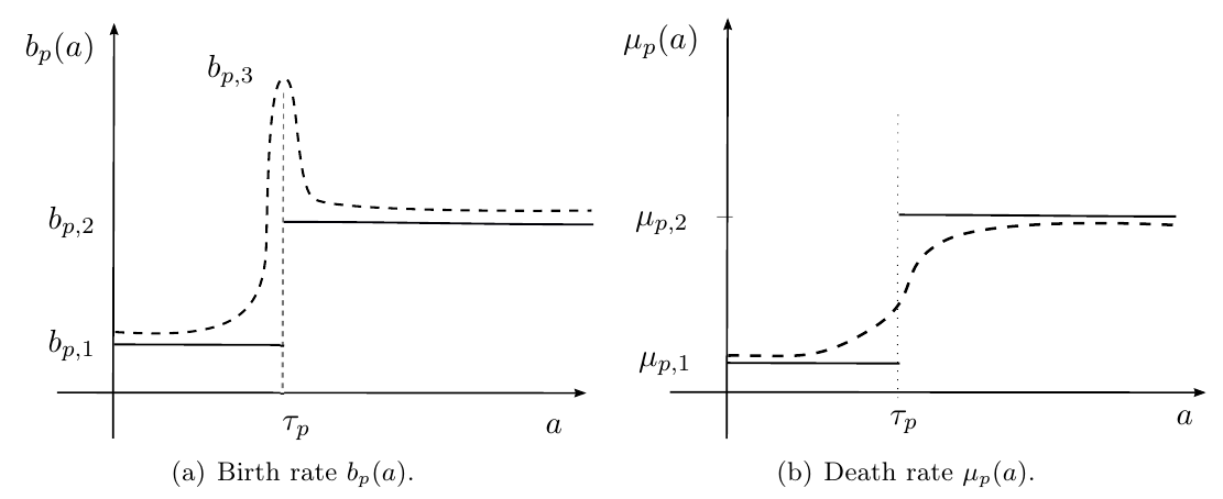
For the age-structured predator population, we choose birth and death rates in the form

$$\mu_{p}(a) =\mu_{p,1}+(\mu_{p,2}-\mu_{p,1})H_{\tau_{p}}(a),$$

$$b_{p}(a) =b_{p,1}+(b_{p,2}-b_{p,1})H_{\tau_{p}}(a)+b_{p,3}\delta_{\tau_{p}}(a),$$

where $H_{\tau_{p}}(a)$ is the Heaviside function with a jump at $a=\tau_{p}$. The coefficients $b_{p,k},\mu_{p,k},\,k=\{1,2\},$ represent birth and death rates of juveniles ($k=1$) and adults ($k=2$). When individuals reach sexual maturity, at age $a=\tau_{p}$, there may be a peak of weight $b_{p,3}\geq 0$ in the fertility rate ($\delta_{\tau_{p}}(a)$ is the delta distribution). A similar assumption was used in [4]. Figure 1 shows the rates $b_{p}(a)$ and $\mu_{p}(a)$.

Figure 1: Birth and death rates of predators are functions of the age $a$. Solid lines reflect the model assumptions, dashed curves represent biologically realistic smooth functions.

Taking into account effects of predation, we put up a modified Lotka-Sharpe model for $p_{1}(a,t)$:

$$\frac{\partial}{\partial t}p_{1}(a,t)+\frac{\partial}{\partial a}p_{1}(a,t) =-\mu_{p}(a)p_{1}(a,t),$$

$$p_{1}(0,t) =\int_{0}^{\infty}b_{p}(a)p(a,t)da$$

$$=\bigl{(}b_{p,1}P_{1}(t)+b_{p,2}P_{2}(t)+b_{p,3}p_{1}(\tau_{p}^{-},t)\bigr{)}h(t),$$

$$p_{1}(a,0) =p_{1}^{0}(a),$$

with $p_{1}^{0}(a)\geq 0$ for all $a\in[0,\tau_{p})$. Assuming that no individual dies at the very moment when it becomes adult, $p_{2}(\tau_{p}^{+},t)=p_{1}(\tau_{p}^{-},t)$, and that $\lim\limits_{a\to\infty}p_{2}(a,t)=0$, we have a similar system for $p_{2}(a,t)$ with initial age distribution $p_{2}^{0}(a)\geq 0$ for all $a>\tau_{p}$.
 
The total number of juvenile individuals satisfies

$$P_{1}^{\prime}(t) =\int_{0}^{\tau_{p}^{-}}\frac{\partial p_{1}}{\partial t}(a,t)\,da\,=\,\int_{0}^{\tau_{p}^{-}}-\frac{\partial p_{1}}{\partial a}(a,t)-\mu_{p,1}p_{1}(a,t)da$$

$$=p_{1}(0,t)-p_{1}(\tau_{p}^{-},t)-\mu_{p,1}P_{1}(t),$$

and for the adult population we have

$$P_{2}^{\prime}(t)=\int_{\tau_{p}{+}}^{\infty}\frac{\partial p_{2}}{\partial t}(a,t)\,da=p_{1}(\tau_{p}^{-},t)-\mu_{p,2}P_{2}(t).$$ (9)

With the explicit solution (6) of a Lotka-Sharpe model, we find for $t<\tau_{p}$

$$p_{1}(\tau_{p}^{-},t)=p_{1}^{0}(\tau_{p}-t)e^{-\mu_{p,1}t},$$

and for $t\geq\tau_{p}$,

$$p_{1}(\tau_{p}^{-},t)=\Bigl{[}b_{p,1}h(t-\tau_{p})P_{1}(t-\tau_{p})+b_{p,2}h(t-\tau_{p})P_{2}(t-\tau_{p})+b_{p,3}h(t-\tau_{p})p_{1}(\tau_{p}^{-},t-\tau_{p})\Bigr{]}e^{-\mu_{p,1}\tau_{p}}.$$

With (9), for $t\geq\tau_{p}$ we have

$$p_{1}(\tau_{p}^{-},t) =\Bigl{[}b_{p,1}h(t-\tau_{p})P_{1}(t-\tau_{p})+b_{p,2}h(t-\tau_{p})P_{2}(t-\tau_{p})$$

$$\phantom{=}+b_{p,3}h(t-\tau_{p})\Bigl{(}P_{2}^{\prime}(t-\tau_{p})+\mu_{p,2}P_{2}(t-\tau_{p})\Bigr{)}\Bigr{]}e^{-\mu_{p,1}\tau_{p}}.$$

For the prey population, we have in general the first equation in (8). One possible choice for $\alpha(R)$ could be the logistic growth with carrying capacity $K>0$ and net growth rate $r>0$,

$$R^{\prime}(t)=\underbrace{r\left(1-\frac{R(t)}{K}\right)}_{\alpha(R(t))}R(t)-g(t)\delta(P_{1}(t),P_{2}(t)).$$ (10)

For $t<\tau_{p}$ the predator population satisfies

$$P_{1}^{\prime}(t) =\bigl{(}b_{p,1}h(t)-\mu_{p,1}\bigr{)}P_{1}(t)+b_{p,2}h(t)P_{2}(t)+\bigl{(}b_{p,3}h(t)-1\bigr{)}p_{1}^{0}(\tau_{p}-t)e^{-\mu_{p,1}t},$$ (11)

$$P_{2}^{\prime}(t) =-\mu_{p,2}P_{2}(t)+p_{1}^{0}(\tau_{p}-t)e^{-\mu_{p,1}t}.$$

For $t\geq\tau_{p}$ we have

$$P_{1}^{\prime}(t) =\bigl{(}b_{p,1}h(t)-\mu_{p,1}\bigr{)}P_{1}(t)+b_{p,2}h(t)P_{2}(t)+\bigl{(}b_{p,3}h(t)-1\bigr{)}b_{p,1}h(t-\tau_{p})P_{1}(t-\tau_{p})e^{-\mu_{p,1}\tau_{p}}$$ (12)

$$\phantom{=}+\bigl{(}b_{p,3}h(t)-1\bigr{)}\Bigl{(}b_{p,2}h(t-\tau_{p})+b_{p,3}h(t-\tau_{p})\mu_{p,2}\Bigr{)}e^{-\mu_{p,1}\tau_{p}}P_{2}(t-\tau_{p})$$

$$\phantom{=}+\bigl{(}b_{p,3}h(t)-1\bigr{)}b_{p,3}h(t-\tau_{p})e^{-\mu_{p,1}\tau_{p}}P_{2}^{\prime}(t-\tau_{p}),$$

$$P_{2}^{\prime}(t) =\Bigl{[}b_{p,1}h(t-\tau_{p})P_{1}(t-\tau_{p})+\Bigl{(}b_{p,2}h(t-\tau_{p})+b_{p,3}h(t-\tau_{p})\mu_{p,2}\Bigr{)}P_{2}(t-\tau_{p})$$

$$\phantom{=\Bigl{[}}+b_{p,3}h(t-\tau_{p})P_{2}^{\prime}(t-\tau_{p})\Bigr{]}e^{-\mu_{p,1}\tau_{p}}-\mu_{p,2}P_{2}(t).$$

We have obtained a class of systems (10), (11), respectively (10), (12), in which we can cast several examples from the literature.
Consider the system for $t\geq\tau_{p}$. For $b_{p,3}=0$, we have a system of the form (8). It is now clear how $m_{1}$ and $\pi_{2}$ should be formulated in terms of $h(t-\tau_{p})$ and $P_{j}(t-\tau_{p}),\,j=1,2$. Assuming that juvenile individuals are not fertile ($b_{p,1}=0$), we obtain

$$R^{\prime}(t) =r\left(1-\frac{R(t)}{K}\right)R(t)-g(t)\delta(P_{1}(t),P_{2}(t)),$$ (13)

$$P_{1}^{\prime}(t) =-\mu_{p,1}P_{1}(t)+b_{p,2}h(t)P_{2}(t)-b_{p,2}h(t-\tau_{p})e^{-\mu_{p,1}\tau_{p}}P_{2}(t-\tau_{p}),$$

$$P_{2}^{\prime}(t) =b_{p,2}h(t-\tau_{p})P_{2}(t-\tau_{p})e^{-\mu_{p,1}\tau_{p}}-\mu_{p,2}P_{2}(t).$$

A proper choice of birth and death rates and of the functions $h$ and $g$ yields, e.g., the model by Gourley and Kuang [10]. Another system of the form (10), (11) is the third model in [19], though there is here no equation for $P_{1}$ (predators are meant to be adult predators). A “complementary” model to (10), (11) is provided in [11], where maturation is considered only for the prey population. In addition our approach shows that sometimes examples from the literature are inconsistent with the biological phenomena. For example Ross [21] suggests a model in which the recruitment into the adult predator population is given by $b_{p,2}R(t)P_{2}(t-\tau_{p})$. Apparently, the delay in the prey density has been neglected.

2.2 Age-structured predator and prey population

Now we assume that the prey population is structured by age, too. As in Section 2.1, we simplify the age structure by introducing an age-at-maturity, $\tau_{r}>0$, for the prey. Again, we shall consider only juvenile and adult individuals. The advantage of an age structure for the prey population is not only that we have age-dependent fertility and mortality rate, but we can also assume that predation depends on the age of the prey. This allows us to include age-specific predation into the model and to reflect different possible settings from biology. In general, a mathematical model which includes juvenile and adult predators (respectively, prey) is an extension of system (8) and can be described by a system of four equations

$$R_{1}^{\prime} =\alpha_{1}(R_{1},R_{2})a_{1}(R_{1},R_{2})-q_{1}(R_{1},R_{2},P_{1},P_{2})-g_{1}(R_{1},R_{2},P_{1},P_{2})\delta_{1}(P_{1},P_{2}),$$

$$R_{2}^{\prime} =\rho_{2}(R_{1},R_{2},P_{1},P_{2})-g_{2}(R_{1},R_{2},P_{1},P_{2})\delta_{2}(P_{1},P_{2}),$$

$$P_{1}^{\prime} =h(R_{1},R_{2},P_{1},P_{2})\beta_{1}(P_{1},P_{2})-m_{1}(R_{1},R_{2},P_{1},P_{2})-\gamma_{1}(P_{1},P_{2})P_{1},$$

$$P_{2}^{\prime} =\pi_{2}(R_{1},R_{2},P_{1},P_{2})-\gamma_{2}(P_{1},P_{2})P_{2}.$$

Here the term $q_{1}$ indicates maturation of juvenile prey and $\rho_{2}$ the recruitment into the adult prey class. As in (8) predation and recruitment rates can be due to all classes of individuals. For simplicity we denote the functions $g_{j}(\cdot)$ and $h(\cdot)$ by $g_{j}(t)$, $j=1,2$, and $h(t)$, respectively.
 
As in Section 2.1 we start with age-structured prey and predator populations and derive DDEs for juvenile and adult individuals. For the predator population we have essentially the systems (11) and (12). Equations for the prey population can be obtained in a similar way, however, we have to take into account age-specific predation. We assume that only adult preys undergo predation, that is $g_{1}(t)\equiv 0$. This assumption fits several insect species, where individuals in the egg and larval stage are well protected [25]. It follows that $q_{1}(R_{1},R_{2},P_{1},P_{2})=q_{1}(R_{1},R_{2})$ and $\rho_{2}(R_{1},R_{2},P_{1},P_{2})=\rho_{2}(R_{1},R_{2})$.
For simplicity of computation, let $g_{2}(t)=\mu_{r,2}R_{2}(t)$ (however a different choice of $g_{2}$ is also possible, cf. Section 1). Under the assumption that juveniles die at constant rate $\mu_{r,1}$, we have

$$\mu_{r}(a) =\mu_{r,1}+\bigl{(}\delta_{2}(P_{1}(t),P_{2}(t))\mu_{r,2}-\mu_{r,1}\bigr{)}H_{\tau}(a).$$

Let $r_{1}(a,t),\,a\in[0,\tau_{r})$ be the density of juvenile prey at time $t\geq 0$. Analogously, $r_{2}(a,t),\,a\in(\tau_{r},\infty)$ denotes the density of adult prey at time $t\geq 0$. Let $R_{1}(t)$ (respectively, $R_{2}(t)$) be the total juvenile (respectively, adult) population size at time $t$.
As in the previous section, we consider the PDE model for $r_{1}(a,t)$ and $r_{2}(a,t)$ and obtain a system of differential equations for $R_{1}$ and $R_{2}$. Computation yields for $t<\tau_{r}$

$$R_{1}^{\prime}(t) =\bigl{(}b_{r,1}-\mu_{r,1}\bigr{)}R_{1}(t)+b_{r,2}R_{2}(t)+\bigl{(}b_{r,3}-1\bigr{)}r_{1}^{0}(\tau_{r}-t)e^{-\mu_{r,1}t},$$ (14)

$$R_{2}^{\prime}(t) =-\mu_{r,2}\delta_{2}(P_{1}(t),P_{2}(t))R_{2}(t)+r_{1}^{0}(\tau_{r}-t)e^{-\mu_{r,1}t},$$

and for $t\geq\tau_{r}$

$$R_{1}^{\prime}(t) =\bigl{(}b_{r,1}-\mu_{r,1}\bigr{)}R_{1}(t)+b_{r,2}R_{2}(t)+\bigl{(}b_{r,3}-1\bigr{)}b_{1}R_{1}(t-\tau_{r})e^{-\mu_{r,1}\tau_{r}}$$ (15)

$$\phantom{=}+\bigl{(}b_{r,3}-1\bigr{)}\Bigl{(}b_{r,2}+b_{r,3}\mu_{r,2}\Bigr{)}e^{-\mu_{r,1}\tau_{r}}R_{2}(t-\tau_{r})$$

$$\phantom{=}+\bigl{(}b_{r,3}-1\bigr{)}b_{r,3}e^{-\mu_{r,1}\tau_{r}}R_{2}^{\prime}(t-\tau_{r}),$$

$$R_{2}^{\prime}(t) =\Bigl{[}b_{r,1}R_{1}(t-\tau_{r})+\Bigl{(}b_{r,2}+b_{r,3}\mu_{r,2}\Bigr{)}R_{2}(t-\tau_{r})$$

$$\phantom{=}+b_{r,3}R_{2}^{\prime}(t-\tau_{r})\Bigr{]}e^{-\mu_{r,1}\tau_{r}}-\mu_{r,2}\delta_{2}(P_{1}(t),P_{2}(t))R_{2}(t).$$

Hence we have obtained a general class of predator-prey systems in which we can cast several examples from the literature (of course a proper choice of birth and death rates and of the functions $h$ and $\delta_{2}$ is necessary). As for the systems (4) and (8), also in this case there is a certain relation between predation response and fecundity response of predators. It is meaningful to choose $h(t)$ proportional to a linear combination of $g_{1}(t)$ and $g_{2}(t)$, that is, the growth rate of predators depends on the (eaten) prey (cf. [19, 13, 3]). If predation is only due to adult predators, then we have $\delta_{j}(P_{1},P_{2})=\delta_{j}(P_{2}),\,j=1,2$.
It is worth noticing that often in previous models no distinction between juvenile and adult individuals has been made (cf. [2, 19, 13]). A comparison with our model suggests that, mostly, heuristically introduced equations describe the dynamics of adult prey and predators. A special case, in which predators and prey species have the same maturation time was given in [19]. Further, when two populations of juveniles and adult individuals are explicitly introduced, e.g., in [10], then usually it is assumed that juvenile individuals are not fertile, that is, $b_{1}=0$ as in (13).
Our approach guarantees that the obtained mathematical model is consistent with biology. This is not the case for all models. For example in [3] death of prey is described by the term $-\mu_{r}P(t)R(t-\sigma)$, whereas recruitment into predator population is given by $bP(t-\tau)R(t)$. The two delays $\sigma$ and $\tau$ seem to have no connection with maturation times and it remains unclear how they should be motivated from a biological point of view.
 
In general, prey and predators are not characterized by the same age-at-maturity, that is, we could have $\tau_{p}\neq\tau_{r}$. Hence, there are three time intervals which we have to consider separately. Let $\tau_{min}:=\min\{\tau_{p},\tau_{r}\}$ and $\tau_{max}:=\max\{\tau_{p},\tau_{r}\}$. For $t\in[0,\tau_{min})$, we have a nonautonomous ODE system (11), (14), whose right-hand side depends on the initial age distribution of the underlying PDE model. For $t\in[\tau_{min},\tau_{max})$, we have a system consisting of two nonautonomous ODEs and two neutral equations with constant delay. If $\tau_{min}=\tau_{p}$, the system is given by (12) – (14), whereas it is given by (11), (15), if $\tau_{min}=\tau_{r}$. In both cases, we have a combination of initial data given by the initial age distribution of the PDE model and the solution of the system on $[0,\tau_{min})$. For $t\in[\tau_{max},\infty)$, we have a system of four neutral equations with two constant delays (12), (15). Here the initial data is given by the solution on $[0,\tau_{max})$.
 
In the general settings presented above, we have assumed that there is a peak of weight $b_{p,3}$ in the birth rate when individuals reach maturity. Such a peak in the fertility rate was observed, e.g., in loggerhead turtles [5], as well as in many insect populations [25]. From a mathematical point of view, $b_{p,3}\neq 0$ yields a neutral equation. To the best of our knowledge, there are only few other examples of neutral equations for predator-prey interactions. Kuang [13] suggests a system with neutral term in the equation for the prey,

$$R^{\prime}(t)=rR(t)\left(1-\frac{R(t-\tau_{r})+\dot{R}(t-\tau_{r})}{K}\right)-P(t)\rho(R(t)).$$ (16)

This model is essentially obtained by extending the “neutral logistic equation” in [9] with a further death term due to predation. The formal derivation of a DDE from the age structure yields in (15) a delay in the recruitment term of the prey, in contrast to equation (16), where the delay appears in the death term (see also [4] for similar observations for single population dynamics).
However, in many species, one does usually not observe a peak in the fertility rate, but rather a jump, when individuals become sexually mature, see e.g. the data set in [18]. In the following we shall neglect the peak in $b(a)$, both for the prey and for the predator population, i.e., $b_{p,3}=0=b_{r,3}$. This assumption reduces the problem to a system of (non-neutral) equations with constant delays.

Symbol	Description
$p(a,t)$	density of predators of age $a$ at time $t$
$p_{j}(a,t)$	density of juvenile/adult predators of age $a$ at time $t$
$P(t)$	size of predator population at time $t$
$P_{j}(t)$	size of juvenile/adult predator population at time $t$
$r(a,t)$	density of prey of age $a$ at time $t$
$r_{j}(a,t)$	density of juvenile/adult prey of age $a$ at time $t$
$R(t)$	size of prey population at time $t$
$R_{j}(t)$	size of juvenile/adult prey population at time $t$
$\tau_{p}$	age at maturity of predator
$\tau_{r}$	age at maturity of prey
$\mu_{p,j}$	death rate of juvenile/adult predator
$b_{p,j}$	fertility rate of juvenile/adult predator
$b_{p,3}$	fertility rate of predator at age $\tau_{p}$
$\mu_{r,j}$	death rate of juvenile/adult prey
$b_{r,j}$	fertility rate of juvenile/adult prey
$b_{r,3}$	fertility rate of prey at age $\tau_{r}$

Table 1: Variables and parameters for the models in Section 2. The indices $j=1$ and $j=2$ indicate juvenile and adult individuals, respectively. All quantities are nonnegative.

3 Analytical Results

Here we provide some analytical results for the model with one delay. Much more challenging is the case of two (or several) delays, which shall be studied in a forthcoming paper.
 
Consider the model (13) for $t\geq\tau_{p}$, and let $g(t)=g(R(t),P_{2}(t))$ and $h(t)=h(R(t),P_{2}(t))$. For simplicity of notation, we omit the $p$-index in the coefficients and in the delay. For $t<\tau$ we have

$$R^{\prime}(t) =r\left(1-\frac{R(t)}{K}\right)R(t)-g(t)\delta(P_{1}(t),P_{2}(t)),$$ (17)

$$P_{1}^{\prime}(t) =-\mu_{1}P_{1}(t)+b_{2}h(t)P_{2}(t)-p_{1}^{0}(\tau-t)e^{-\mu_{1}t},$$ (18)

$$P_{2}^{\prime}(t) =-\mu_{2}P_{2}(t)+p_{1}^{0}(\tau-t)e^{-\mu_{1}t}.$$ (19)

Taken together the model, which describes the dynamics in the whole interval $[0,\infty)$ can be seen as a general formulation of the system by Gourley and Kuang [10].
 
Preservation of positivity is a crucial factor in mathematical biology. However, systems of DDEs can possibly have negative solutions even when the initial functions are nonnegative [23]. In the following we provide criteria to guarantee nonnegative solutions of (13).
The right-hand side of (17)–(19) depends on the initial age distribution $p^{0}_{1}(a)$ of a PDE system of the form (5) for the juvenile predator. If $p^{0}_{1}(a)\geq 0,\,a\geq 0$ is known, we take the solution of (17)–(19) as history function for (13) and we obtain nonnegative solutions. Now consider the case in which $p^{0}_{1}(a)$ is not known. Following [4], we start with (19) and find

$$\frac{d}{dt}\bigl{(}P_{2}(t)e^{\mu_{2}t}\bigr{)}e^{(\mu_{1}-\mu_{2})t} =p_{1}^{0}(\tau-t)\qquad(\geq 0).$$

That is, the function $P_{2}(t)e^{\mu_{2}t}$ is nondecreasing on $[0,\tau]$. Integration in $[0,\tau]$ yields

$$P_{1}(0)=P_{2}(\tau)e^{\mu_{1}\tau}-P_{2}(0)-(\mu_{1}-\mu_{2})\int_{0}^{\tau}P_{2}(t)e^{\mu_{1}t}dt.$$ (20)

We use (18) to substitute the term $p_{1}^{0}(\tau-t)e^{-\mu_{1}t}$ and obtain

$$P_{1}^{\prime}(t) =-\mu_{1}P_{1}(t)+\bigl{(}b_{2}h(t)-\mu_{2}\bigr{)}P_{2}(t)-P_{2}^{\prime}(t).$$

The last equation can be solved with variation of constants and integration by parts,

$$P_{1}(t) =\bigl{(}P_{1}(0)+P_{2}(0)\bigr{)}e^{-\mu_{1}t}-P_{2}(t)+\int_{0}^{t}\bigl{(}b_{2}h(s)-\mu_{2}\bigr{)}P_{2}(s)e^{\mu_{1}(s-t)}ds$$ (21)

$$\phantom{=}\;+\mu_{1}\int_{0}^{t}P_{2}(s)e^{\mu_{1}(s-t)}ds.$$

As the equation (17) is an ODE, there is no problem with positivity of solutions, as long as we choose a nonnegative initial value $R(0)$. The solution exists and is unique, given continuously differentiable $g$ and $\delta$.
We define an operator $T:(C[0,\tau])^{2}\rightarrow C[0,\tau]$ so that $(T(R,P_{2}))(t)=P_{1}(t)$ for $t\in[0,\tau]$ and $P_{1}(t)$ is given by (21) with $P_{1}(0)$ as in (20). The cone $\mathcal{K}$ is defined by

$$\mathcal{K}:= \Bigl{\{}(R,P_{1},P_{2})\in(C[0,\tau])^{3}:\;P_{2}(0)\geq 0,$$

$$\phantom{==}P_{2}(t)e^{\mu_{2}t}\text{ is nondecreasing in }[0,\tau],\;P_{1}=T(R,P_{2}),R(0)\geq 0\Bigr{\}}.$$

Proposition 3.1.

Let a PDE system of the form (5) for $p_{1}(a,t)$ be given with initial age distribution $p_{1}^{0}(a)\geq 0$. Then the functions $R(t),P_{1}(t),P_{2}(t)$ defined in Section 2.1 satisfy system (17)–(19) and $(R,P_{1},P_{2})\big{|}_{[0,\tau]}\in\mathcal{K}$.
 
Conversely, for $(\tilde{R},\tilde{P}_{1},\tilde{P}_{2})\in\mathcal{K}$, there is an initial age distribution $p_{1}^{0}(a)\geq 0$ such that the solution $(R,P_{1},P_{1})$ of the system (17)–(19) satisfies $(R,P_{1},P_{2})\big{|}_{[0,\tau]}=(\tilde{R},\tilde{P}_{1},\tilde{P}_{2})$.

Proof. The first part has already been shown. The rest of the proof follows similar to [4], with the difference that here the operator $T$ has two arguments.

3.1 Linearised stability

3.1.1 The case $\tau=0$

First we consider (13) with $\tau=0$. From a biological point of view, this means that newborn individuals are sexually mature. The juvenile class $P_{1}$ loses its original meaning. Evidently, $\lim\limits_{t\to\infty}P_{1}(t)=0$. Fixed points of the system are the trivial equilibrium $E_{0}=(0,0,0)$, in which we find neither prey nor predator, the point $E_{R}=(K,0,0)$, where only prey are present and a coexistence equilibrium $E_{C}=(R^{*},0,P_{2}^{*})$, with $R^{*}\in(0,K)$ and $P_{2}^{*}>0$. Such an equilibrium is obtained as the intersection of the curve $b_{2}h(R^{*},P_{2}^{*})=\mu_{2}$ and the prey isocline $rR^{*}(1-\frac{R^{*}}{K})=g(R^{*},P_{2}^{*})\delta(0,P_{2}^{*})$ in the positive cone. The number of coexistence points depends on the choice of the functions $h$ and $g$.
 
We denote by $g_{R}$ and $g_{P_{2}}$ the derivative of $g$ with respect to $R$ and ${P_{2}}$, respectively (analogously for $h$). The biology suggests that the functions $h$ and $g$ are nondecreasing both in $P_{2}$ and $R$, hence all the partial derivatives are nonnegative. This assumption includes the possibility that, when the prey population has reached its carrying capacity, the prey dies for reasons different than predation, e.g., external harvesting or migration. However, we assume that $g_{R}(R,0)=0$, for all $R\geq 0$, i.e., in absence of predators no prey dies. The function $\delta(P_{1},P_{2})$ is nondecreasing in both components.

Proposition 3.2.

The trivial equilibrium $E_{0}=(0,0,0)$ is always unstable.
The point $E_{R}=(K,0,0)$ is locally asymptotically stable if $\mu_{2}>b_{2}h(K,0)$.

Proof. The proof follows with standard linear stability theory. Computation can be found in [16].
 
Consider the coexistence equilibrium $E_{C}=(R^{*},0,P_{2}^{*})$. As the $P_{1}$-direction is always stable, it is sufficient to investigate the matrix $A=\left(a_{l,k}\right)_{l,k=1,2}$,

$$A=\begin{pmatrix}r-2\frac{r}{K}R^{*}-g_{R}(R^{*},P_{2}^{*})\delta(0,P_{2}^{*})&-g_{P_{2}}(R^{*},P_{2}^{*})\delta(0,P_{2}^{*})-g(R^{*},P_{2}^{*})\delta_{P_{2}}(0,P_{2}^{*})\\ &\\ b_{2}h_{R}(R^{*},P_{2}^{*})P_{2}^{*}&b_{2}h_{P_{2}}(R^{*},P_{2}^{*})P_{2}^{*}\end{pmatrix}.$$

Notice that $a_{1,2}\leq 0$, whereas $a_{2,1}$ and $a_{2,2}$ are nonnegative. The coexistence point is stable when $\det(A)>0$ and $\operatorname{trace}(A)<0$.

3.1.2 The case $\tau>0$

As in the case $\tau=0$ we have the equilibria $E_{0}=(0,0,0)$ and $E_{R}=(K,0,0)$. Coexistence equilibria depend on the choice of $h$ and $g$. In Section 3.2 we show an example in which the coexistence point $E_{C}=(R^{*},P_{1}^{*},P_{2}^{*})$ is uniquely determined. We say a coexistence point is feasible when it is in the positive cone and all its components are bounded.
 
Linearised stability analysis [23] allows to reduce the problem to a standard linear equation of the form $x^{\prime}(t)=Ax(t)+Bx(t-\tau)$. It is immediate to prove that the delay has no influence on the stability of the trivial equilibrium $E_{0}$. It is locally asymptotically stable if $r<g_{R}(0,0)\delta(0,0)$ holds, otherwise unstable [16].
Linearisation about the point $E_{R}$ yields the characteristic equation

$$\bigl{(}\lambda+r+g_{R}(K,0)\delta(0,0)\bigr{)}\bigl{(}\lambda+\mu_{1}\bigl{)}\bigl{(}\lambda+\mu_{2}-e^{-(\mu_{1}+\lambda)\tau}b_{2}h(K,0)\bigr{)}=0.$$

The characteristic roots are $\lambda_{1}=-r-g_{R}(K,0)\delta(0,0)\in\mathbb{R},\,\lambda_{2}=-\mu_{1}\in\mathbb{R}$ and $\lambda_{3}$ which is given by the equation

$$\lambda+\mu_{2}-e^{-(\mu_{1}+\lambda)\tau}b_{2}h(K,0)=0.$$ (22)

This equation has the form $\lambda-a-be^{-\tau\lambda}=0,$ with $a=-\mu_{2}$ and $b=e^{-\mu_{1}\tau}b_{2}h(K,0)>0$ for all $\tau>0$. The delay in the coefficients of the characteristic equation can make the stability analysis challenging. However, Theorem 6 in [8] ensures that equation (22) has a real dominant root (the condition $-e^{-1}\leq b\tau e^{-a\tau}$ holds for all $\tau>0$). Hence it is sufficient to investigate the real characteristic roots of (22), which are given by the intersections of the line $y=x+\mu_{2}$ with the curve $y=b_{2}h(K,0)e^{-\mu_{1}\tau}e^{-x\tau}$.

Proposition 3.3.

The equilibrium $E_{R}$ of system (13) is locally asymptotically stable if it holds that

$$r+g_{R}(K,0)\delta(0,0)>0\qquad\mbox{and}\qquad\mu_{2}>b_{2}h(K,0)e^{-\mu_{1}\tau}.$$

Assume that there is a uniquely determined coexistence point $E_{C}=(R^{*},P_{1}^{*},P_{2}^{*})$. For simplicity of computation we assume that predation is only due to adult predators, i.e., $\delta(P_{1},P_{2})=\delta(P_{2})$. We are interested in stability properties of $E_{C}$ with respect to the delay $\tau>0$. To this purpose we shall make use of results in [3, Sec. 2]. Linearisation of (13) about $E_{C}$ yields the characteristic equation $G(\lambda;\tau)=0$, with

$$G(\lambda;\tau) =\bigl{(}\lambda+\mu_{1}\bigr{)}\Bigl{[}\Bigl{(}\lambda+\mu_{2}-e^{-(\lambda+\mu_{1})\tau}\bigl{(}b_{2}h(R^{*},P_{2}^{*})+b_{2}h_{P_{2}}(R^{*},P_{2}^{*})P_{2}^{*}\bigr{)}\Bigr{)}$$

$$\;\phantom{=}\cdot\Bigl{(}\lambda-r+2\frac{rR^{*}}{K}+g_{R}(R^{*},P_{2}^{*})\delta(P_{2}^{*})\Bigr{)}$$

$$\phantom{=}+e^{-(\lambda+\mu_{1})\tau}b_{2}h_{R}(R^{*},P_{2}^{*})P_{2}^{*}\Bigl{(}g_{P_{2}}(R^{*},P_{2}^{*})\delta(P_{2}^{*})+g(R^{*},P_{2}^{*})\delta^{\prime}(P_{2}^{*})\Bigr{)}\Bigr{]}.$$

Hence we have one real root $\lambda=-\mu_{1}$, whereas other roots are determined by the term in the square brackets. The above characteristic equation can be written in the form

$$P(\lambda;\tau)+Q(\lambda;\tau)e^{-\lambda\tau}=0,$$

with

$$P(\lambda;\tau) =\lambda^{2}+\left(2\frac{r}{K}R^{*}+g_{R}(R^{*},P_{2}^{*})\delta(P_{2}^{*})-r+\mu_{2}\right)\lambda$$

$$\phantom{=}+\left(2\frac{r}{K}R^{*}+g_{R}(R^{*},P_{2}^{*})\delta(P_{2}^{*})-r\right)\mu_{2},$$

$$Q(\lambda;\tau) =-e^{-\mu_{1}\tau}\left(b_{2}h(R^{*},P_{2}^{*})+b_{2}h_{P_{2}}(R^{*},P_{2}^{*})P_{2}^{*}\right)\lambda$$

$$\phantom{=}-e^{-\mu_{1}\tau}\biggl{[}\left(b_{2}h_{R}(R^{*},P_{2}^{*})+b_{2}h_{P_{2}}(R^{*},P_{2}^{*})P_{2}^{*}\right)\left(2\frac{r}{K}R^{*}+g_{R}(R^{*},P_{2}^{*})\delta(P_{2}^{*})-r\right)$$

$$\phantom{=}-b_{2}h_{R}(R^{*},P_{2}^{*})\left(g_{P_{2}}(R^{*},P_{2}^{*})\delta(P_{2}^{*})+g(R^{*},P_{2}^{*})\delta^{\prime}(P_{2}^{*})\right)P_{2}^{*}\biggr{]}.$$

Let

$$\beta =2\frac{r}{K}R^{*}+g_{R}(R^{*},P_{2}^{*})\delta(P_{2}^{*})-r,$$ (23)

$$\gamma =b_{2}h(R^{*},P_{2}^{*})+b_{2}h_{P_{2}}(R^{*},P_{2}^{*})P_{2}^{*},$$

$$\varepsilon =b_{2}h_{R}(R^{*},P_{2}^{*})\Bigl{(}g_{P_{2}}(R^{*},P_{2}^{*})\delta(P_{2}^{*})+g(R^{*},P_{2}^{*})\delta^{\prime}(P_{2}^{*})\Bigr{)}P_{2}^{*},$$

and obtain

$$P(\lambda;\tau)=\lambda^{2}+(\beta+\mu_{2})\lambda+\mu_{2}\beta,\qquad Q(\lambda;\tau)=-e^{-\mu_{1}\tau}\gamma\lambda-e^{-\mu_{1}\tau}\bigl{(}\gamma\beta-\varepsilon\bigr{)}.$$

Stability properties of $E_{C}$ are determined by the real part of the characteristic roots. Define the functions

$$M:[0,\infty)\to\mathbb{R}, \;\;\tau\,\mapsto\,\beta^{2}+\mu_{2}^{2}-e^{-2\mu_{1}\tau}\gamma^{2},$$

$$N:[0,\infty)\to\mathbb{R}, \;\;\tau\,\mapsto\,e^{-2\mu_{1}\tau}(\gamma\beta-\varepsilon)^{2}-\mu_{2}^{2}\beta^{2}.$$

As the delay appears in the coefficients of the characteristic equation (notice that $\tau$ is also in the coordinates of the point $E_{C}$) it is difficult to determine precisely the value of the delay at which stability switches occur. However, we have the following result.

Theorem 3.1.

Let $\beta\bigl{(}\gamma-\mu_{2}e^{\mu_{1}\tau}\bigr{)}\neq\varepsilon$ with $\tau\geq 0$. The stability of $E_{C}$ depends on the value of the delay $\tau\geq 0$ as follows.

1. Assume $M(\tau)\geq 0$. If $\tau$ increases and enters $S_{c}:=\left\{\tau\in\mathbb{R}_{0}:M(\tau)\geq 0,\;N(\tau)>0\right\}$, stability switches may occur as $\tau$ increases within $S_{c}$. If $\tau\notin S_{c}$, no stability switch occurs.

2. Assume $M(\tau)<0$. If $\tau$ increases and enters $S_{c}:=\left\{\tau\in\mathbb{R}_{0}:M(\tau)<0,\;N(\tau)\geq-\frac{M(\tau)^{2}}{4}\right\}$, stability switches may occur as $\tau$ increases within $S_{c}$. If $\tau\notin S_{c}$, no stability switch occurs.

Proof. We verify the hypothesis of [3, Sec. 2]. The functions $P$ and $Q$ do not have any common imaginary root $\lambda=\pm iy,\;y\in\mathbb{R}_{+}$. Indeed

$$P(iy;\tau)=-y^{2}+i(\beta+\mu_{2})y+\mu_{2}\beta\,=\,0\,=\,-e^{-\mu_{1}\tau}\left(i\gamma y+\gamma\beta-\varepsilon\right)=Q(iy;\tau)$$

only for $y=0$. Further we have $\overline{P(-iy,\tau)}=P(iy,\tau)$ and $\overline{Q(-iy,\tau)}=Q(iy,\tau)$ for $y\in\mathbb{R}$ and for all $\tau\geq 0$. Observe that

$$P(0;\tau)+Q(0;\tau)=\beta\left(\mu_{2}-\gamma e^{-\mu_{1}\tau}\right)-\varepsilon e^{-\mu_{1}\tau}\neq 0,\qquad\mbox{for all}\,\tau\geq 0.$$

Some computation (see [16]) shows that for all $\tau\geq 0$,

$$\limsup\{|Q(\lambda,\tau)|/|P(\lambda,\tau)|:|\lambda|\rightarrow\infty,\Re(\lambda)\geq 0\}<1.$$

Consider purely imaginary roots $\lambda=iy$ for $y\in\mathbb{R}_{+}$. Then we have

$$P_{R}:=\Re(P(iy;\tau))=\mu_{2}\beta-y^{2}, \qquad P_{I}:=\Im(P(iy;\tau))=(\beta+\mu_{2})y,$$

$$Q_{R}:=\Re(Q(iy;\tau))=-e^{-\mu_{1}\tau}\bigl{(}\gamma\beta-\varepsilon\bigr{)}, \qquad Q_{I}:=\Im(Q(iy;\tau))=-e^{-\mu_{1}\tau}\gamma y.$$

Hence,

$$F(y;\tau)\,=\,P_{R}^{2}+P_{I}^{2}-Q_{R}^{2}-Q_{I}^{2}\,=\,y^{4}+M(\tau)y^{2}-N(\tau).$$

With $z:=y^{2}$, the zeros of $F(y;\tau)$ are given by $y_{1,2}=\sqrt{z_{\pm}}$ and $y_{3,4}=-\sqrt{z_{\pm}}$, where

$$z_{\pm}=-\frac{M(\tau)}{2}\pm\sqrt{\frac{M(\tau)^{2}}{4}+N(\tau)}.$$

For each $\tau\geq 0$ we have at most four different real roots of $F(y;\tau)$, hence also the last hypothesis is satisfied. We search for values of $\tau$ such that $F$ has at least one strictly positive root. If $M(\tau)\geq 0$, $z_{-}$ is always negative or complex, but $z_{+}>0$ if and only if $N(\tau)>0$. If $M(\tau)<0$, $z_{-}>0$ if and only of $N(\tau)>0$ and $z_{+}>0$ if and only if $N(\tau)\geq-\frac{M(\tau)^{2}}{4}$.

3.2 A Rosenzweig-MacArthur DDE model

An example for the class of problems (13) is given by a delayed version of the Rosenzweig-MacArthur model (3). We choose the functions $h(t)=h(R(t))=R(t)/(1+R(t))$, $g(t)=g(R(t))=bh(t),\,b>0$, and $\delta(P_{1}(t),P_{2}(t))=\delta(P_{2}(t))=P_{2}(t)$. Notice that these are all $C^{1}$-functions and that $h(0)=0=g(0)$. As observed in the previous section, the $P_{1}$-equation is not relevant for the dynamics of the whole system. Hence, we focus on the system

$$R^{\prime}(t) =R(t)\left(1-\frac{R(t)}{K}\right)-b\frac{R(t)}{1+R(t)}P_{2}(t),$$ (24)

$$P_{2}^{\prime}(t) =-\mu P_{2}(t)+b\frac{R(t-\tau)}{1+R(t-\tau)}P_{2}(t-\tau)e^{-\mu_{1}\tau}.$$

Assume that we have nonnegative continuous initial data $R(\vartheta),P_{2}(\vartheta)$ on $-\tau\leq\vartheta\leq 0$. Then it is easy to proof that the solutions $(R(t),P_{2}(t))$ of (24) are nonnegative for all $t\geq 0$ [16].
 
In the case $\tau=0$, the dynamics of (24) is known [20]. Beside the trivial equilibrium, which always exists, system (24) has a unique coexistence equilibrium $E_{C}=(R^{*},P_{2}^{*})$ with

$$R^{*}=\frac{\mu}{b-\mu},\quad P_{2}^{*}=\frac{1}{b-\mu}\left(1-\frac{\mu}{K(b-\mu)}\right).$$

The coexistence equilibrium is feasible only if $b>\mu$ and $K>K^{*}_{0}=\frac{\mu}{b-\mu}$. The point $E_{C}$ is locally asymptotically stable if $K<\frac{b+\mu}{b-\mu}$, a Hopf bifurcation occurs at $K^{*}_{1}=\frac{b+\mu}{b-\mu}$ and the point becomes unstable.
 
In the case $\tau>0$, for $b>\mu e^{\mu_{1}\tau}$ and $K<\frac{\mu}{be^{-\mu_{1}\tau}-\mu}$, there is only one nontrivial equilibrium $E_{R}=(K,0)$, which is stable for all $\tau\geq 0$. For $b>\mu e^{\mu_{1}\tau}$ and $K>\frac{\mu}{be^{-\mu_{1}\tau}-\mu}$ beside $E_{R}=(K,0)$, we find a unique coexistence point $E_{C}=\left(\frac{\mu}{be^{-\mu_{1}\tau}-\mu},\frac{1}{b}\Bigl{(}1-\frac{R^{*}}{K}\Bigr{)}(1+R^{*})\right)$, whose stability depends on $\tau$. We determine the set $S_{c}$ in which stability switches can occur. With (23) we find the values

$$\beta=\frac{2\mu}{K(be^{-\mu_{1}\tau}-\mu)}-e^{\mu_{1}\tau}\left(\frac{\mu}{b}+\frac{\mu}{Kb}\right),\qquad\gamma=\mu e^{\mu_{1}\tau},\qquad\varepsilon=\mu e^{\mu_{1}\tau}\left[1-e^{\mu_{1}\tau}\left(\frac{\mu}{b}+\frac{\mu}{Kb}\right)\right],$$

and we have that $M(\tau)=\beta^{2}\geq 0$. Hence, stability switches occur for $\tau\geq 0$ such that $N(\tau)>0$, or equivalently for $\tau>0$ such that

$$\varepsilon-2\mu e^{\mu_{1}\tau}\beta>0\quad\Leftrightarrow\quad 1+e^{\mu_{1}\tau}\Bigl{(}\frac{\mu}{b}+\frac{\mu}{Kb}\Bigr{)}-\frac{4\mu}{K(be^{-\mu_{1}\tau}-\mu)}>0.$$

That is, we want to find values $x>0$ such that

$$x^{2}+\frac{3b}{\mu(1+K)}x-\frac{Kb^{2}}{\mu^{2}(1+K)}<0$$ (25)

holds. Zeros of (25) are

$$x_{\pm}=-\frac{3b}{2\mu(1+K)}\pm\sqrt{\frac{9b^{2}}{4\mu^{2}(1+K)^{2}}+\frac{Kb^{2}}{\mu^{2}(1+K)}}.$$

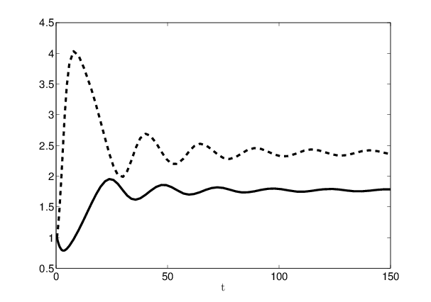
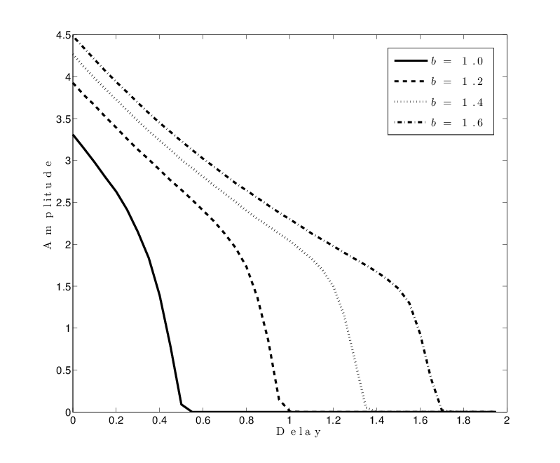
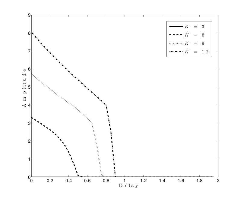
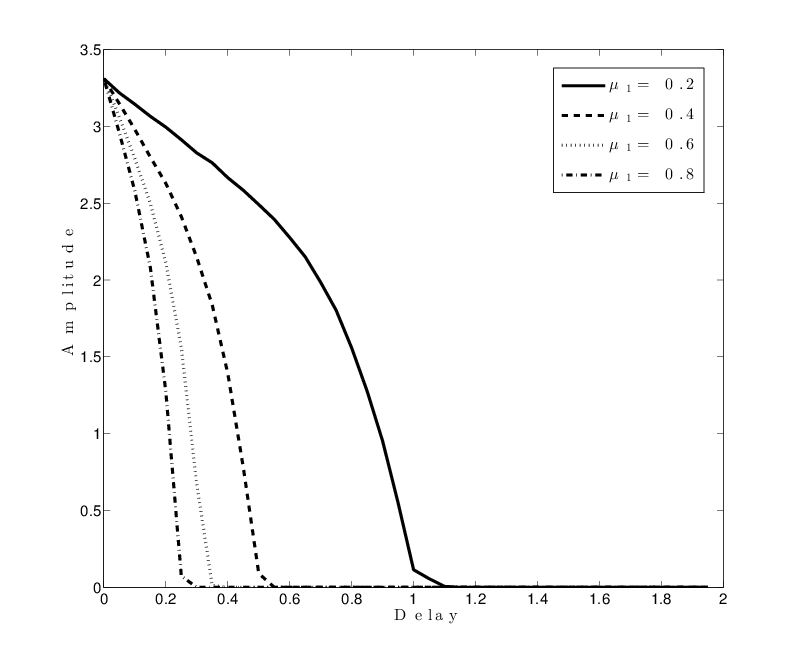
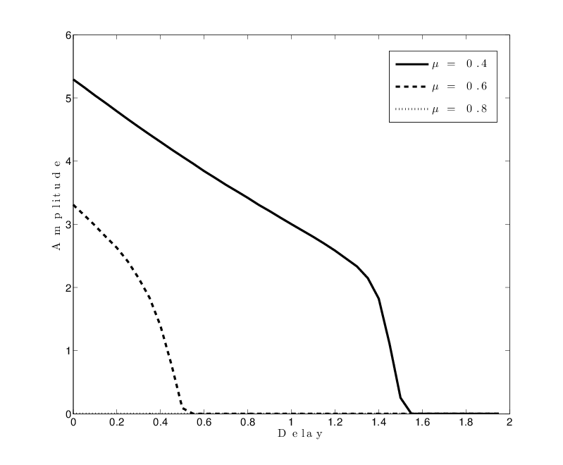
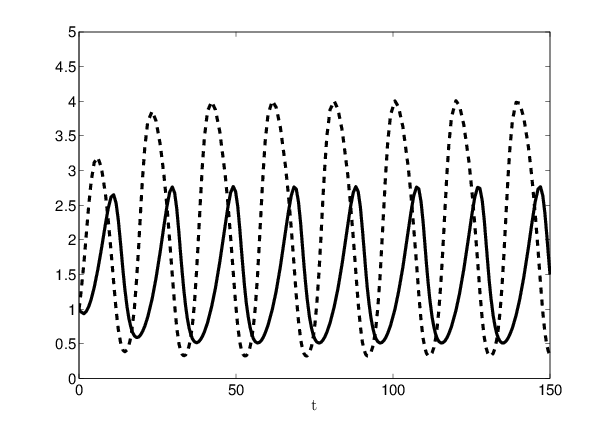
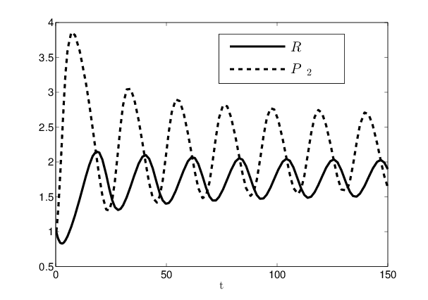
It is easy to see that $x_{-}<0$. Thus $N(\tau)>0$ holds for all $\tau\in S_{c}=[0,\tau_{max})$, with $\tau_{max}=\ln(x_{+})/\mu_{1}$. For $\tau\in[0,\tau_{max})$ we can observe stability switches, for $\tau>\tau_{max}$ the stability of the coexistence point does not change when $\tau$ changes. An example is shown in Figure 2. We observe that both $K$ and $\tau$ can be chosen as bifurcation parameters for (24). For $\tau=0$ and $K\in(0,K^{*}_{0})$ the point $E_{R}$ is stable, whereas for $K\in(K^{*}_{0},K^{*}_{1})$ the coexistence equilibrium $E_{C}$ is locally asymptotically stable and when the carrying capacity $K$ becomes larger than $K^{*}_{1}$ a limit cycle appears. The inclusion into the model of a maturation delay seems to shift forward the destabilization of the equilibria. That is, for $\tau>0$ and $K\in(0,K^{*}_{R}(\tau))$, with $K^{*}_{R}(\tau)\leq K^{*}_{R}(0)=K^{*}_{0}$ the point $E_{R}$ is stable, whereas for $K\in(K^{*}_{R}(\tau),K^{*}_{C}(\tau))$ with $K^{*}_{C}(\tau)\leq K^{*}_{C}(0)=K^{*}_{1}$ the coexistence equilibrium $E_{C}$ is locally asymptotically stable. However, for $K>K^{*}_{C}(\tau)$ an increase in the delay can lead to damped oscillations and again to a stable coexistence equilibrium, cf. Figure 2. A last numerical test shows how periodic solutions depend on the delay and on the other parameters. We consider periodic solutions and compute oscillation amplitudes (over one period of the periodic solution). Figure 3 shows oscillation amplitudes for the solution $P_{2}$ in dependence of the delay and of one other parameters. Observe that there is no periodic solution for very large values of the delay. From a biological point of view, a very large age-at-maturity implies that predators stay long in the juvenile phase and it takes a long time for them to become active predators. During this time the prey can increase and reach a certain density such that the predation effects are not very relevant. This leads to a stable coexistence of predators and prey, rather than the well-known oscillatory dynamics.

(a) $\tau=0.01$.

(b) $\tau=0.3$.

(c) $\tau=0.4$.

Figure 2: Effect of the delay on the solution of the system (24). Numerical simulations were performed with the MATLAB®  solver dde23. For this simulations we choose $K=5,\,b=1,\mu=0.6,\mu_{1}=0.4$ and three values of the delay $\tau$. We may observe stability switches for $\tau\in[0,\tau_{max})$, with $\tau_{max}=0.3728$.

Figure 3: Oscillation amplitudes of the $P_{2}$ population with respect to the delay and one of the parameters. Unless otherwise indicated in the plot, parameter values are $K=6,\,b=1,\mu=0.6,\mu_{1}=0.4$.

References

• [1] P. A. Abrams and L. R. Ginzburg. The nature of predation: prey dependent, ratio dependent or neither? Trends Ecol. Evol., 15(8):337–341, 2000.
• [2] M. S. Bartlett. On theoretical models for competitive and predatory biological systems. Biometrika, 44(1-2):27–42, 1957.
• [3] E. Beretta and Y. Kuang. Geometric stability switch criteria in delay differential systems with delay dependent parameters. SIAM J. Math. Anal., 33(5):1144–1165, 2002.
• [4] G. A. Bocharov and K. P. Hadeler. Structured population models, conservation laws, and delay equations. J. Diff. Equa., 168(1):212–237, 2000.
• [5] D. T. Crouse, L. B. Crowder, and H. Caswell. A stage-based population model for loggerhead sea turtles and implications for conservation. Ecology, 68(5):1412–1423, 1987.
• [6] J. M. Cushing and M. Saleem. A predator prey model with age structure. J. Math. Biol., 14(2):231–250, 1982.
• [7] L. Edelstein-Keshet. Mathematical Models in Biology. SIAM, New York, 1988.
• [8] M. V. S. Frasson. On the dominance of roots of characteristic equations for neutral functional differential equations. Appl. Math. Comput., 214(1):66–72, 2009.
• [9] K. Gopalsamy and B. G. Zhang. On a neutral delay logistic equation. Dynam. Stabil. Syst., 2:183–195, 1988.
• [10] S. A. Gourley and Y. Kuang. A stage structured predator-prey model and its dependence on maturation delay and death rate. J. Math. Biol., 49(2):188–200, 2004.
• [11] A. Hastings. Age-dependent predation is not a simple process. I. continuous time models. Theor. Popul. Biol., 23(3):347–362, 1983.
• [12] A. Hastings. Delays in recruitment at different trophic levels: Effects on stability. J. Math. Biol., 21:35–44, 1984.
• [13] Y. Kuang. On neutral delay logistic gause-type predator-prey systems. Dynam. Stabil. Syst., 6(2):173–189, 1991.
• [14] A. J. Lotka. Elements of physical biology. Williams & Wilkins, Princeton, N. J., 1925.
• [15] R. May. Complexity and stability in model ecosystems. Princeton University Press, 1973.
• [16] M. Mohr. On Predator-Prey Models with Delay due to Maturation. Master’s thesis, Technische Universität München, Munich, 2012.
• [17] R. M. Nisbet and W. S. C. Gurney. The systematic formulation of population models for insects with dynamically varying instar duration. Theor. Popul. Biol., 23(1):114–135, 1983.
• [18] V. N. Novoseltsev, J. A. Novoseltseva, and A. I. Yashin. What does a fly’s individual fecundity pattern look like? The dynamics of resource allocation in reproduction and ageing. Mech. Ageing Dev., 124(5):605–617, 2003.
• [19] L. Nunney. The effect of long time delays in predator-prey systems. Theor. Popul. Biol., 27:202–221, 1985.
• [20] M. L. Rosenzweig and R. H. MacArthur. Graphical representation and stability conditions of predator-prey interactions. Am. Nat., pages 209–223, 1963.
• [21] G. G. Ross. A difference-differential model in population dynamics. J. Theor. Biol., 37(3):477–492, 1972.
• [22] F. R. Sharpe and A. J. Lotka. A problem in age distribution. Philos. Mag. Ser. 6, 21:435–438, 1911.
• [23] H. Smith. An Introduction to Delay Differential Equations with Applications to the Life Sciences. Springer, New York, 2011.
• [24] V. Volterra. Variazioni e fluttuazioni del numero d’individui in specie conviventi. Mem. Accad. Lincei Roma, 2:31–113, 1926.
• [25] K. S. Williams and C. Simon. The ecology, behavior, and evolution of periodical cicadas. Annu. Rev. Entomol., 40(1):269–295, 1995.