Parallel Triangle Counting in Massive Streaming Graphs

Abstract

The number of triangles in a graph is a fundamental metric, used in social network analysis, link classification and recommendation, and more. Driven by these applications and the trend that modern graph datasets are both large and dynamic, we present the design and implementation of a fast and cache-efficient parallel algorithm for estimating the number of triangles in a massive undirected graph whose edges arrive as a stream. It brings together the benefits of streaming algorithms and parallel algorithms. By building on the streaming algorithms framework, the algorithm has a small memory footprint. By leveraging the paralell cache-oblivious framework, it makes efficient use of the memory hierarchy of modern multicore machines without needing to know its specific parameters. We prove theoretical bounds on accuracy, memory access cost, and parallel runtime complexity, as well as showing empirically that the algorithm yields accurate results and substantial speedups compared to an optimized sequential implementation.

(This is an expanded version of a CIKM’13 paper of the same title.)

1 Introduction

The number of triangles in a graph is an important metric in social network analysis [31, 23], identifying thematic structures of networks [10], spam and fraud detection [1], link classification and recommendation [29], among others. Driven by these applications and further fueled by the growing volume of graph data, the research community has developed many efficient algorithms for counting and approximating the number of triangles in massive graphs. There have been several streaming algorithms for triangle counting, including [6, 14, 3, 22, 18, 25, 15]. Although these algorithms are well-suited for handling graph evolution, they cannot effectively utilize parallelism beyond the trivial “embarrassingly parallel” implementation, leaving much to be desired in terms of performance (we further discuss this below). On the other hand, there have been a number of parallel algorithms for triangle counting, such as [27, 9]. While these algorithms excel at processing static graphs using multiple processors, they cannot efficiently handle constantly changing graphs. Yet, despite indications that modern graph datasets are both massive and dynamic, none of the existing algorithms can efficiently handle graph evolution and fully utilize parallelism at the same time.

In this paper, we present a fast shared-memory parallel algorithm for approximate triangle counting in a high-velocity streaming graph. Using streaming techniques, it only has to store a small fraction of the graph but is able to process the graph stream in a single pass. Using parallel-computing techniques, it was designed for modern multicore architecture and can take full advantage of the memory hierarchy. The algorithm is versatile: It can be used to monitor a streaming graph where high throughput and low memory consumption are desired. It can also be used to process large static graphs, reaping the benefits of parallelism and small memory footprints. As is standard, our algorithm provides a randomized relative-error approximation to the number of triangles: given $\varepsilon,\delta\in[0,1]$, the estimate $\hat{X}$ is an $(\varepsilon,\delta)$-approximation of the true quantity $X$ if $|\hat{X}-X|\leq\varepsilon X$ with probability at least $1-\delta$.

We have used the following principles to guide our design and implementation: First, we work in the limited-space streaming model, where only a fraction of the graph can be retained in memory. This allows the algorithm to process graphs much larger than the available memory. Second, we adopt the bulk arrival model. Instead of processing a single edge at a time, our algorithm processes edges one batch at a time. This allows for processing the edges of a batch in parallel, which results in higher throughput. Third but importantly, we optimize for the memory hierarchy. The memory system of modern machines has unfortunately become highly sophisticated, consisting of multiple levels of caches and layers of indirection. Navigating this complex system, however, is necessary for a parallel implementation to be efficient. To this end, we strive to minimize cache misses. We design our algorithm in the so-called cache-oblivious framework [11, 5], allowing the algorithm to make efficient use of the memory hierarchy but without knowing the specific memory/cache parameters (e.g., cache size, line size).

Basic Parallelization: Before delving further into our algorithm, we discuss two natural parallelization schemes and why they fall short in terms of performance. For the sake of this discussion, we will compare the PRAM-style (theoretical) time to process a stream of $m$ total edges on $p$ processors, assuming a reasonable scheduler.

As a concrete running example, we start with the sequential triangle counting algorithm in [25], which uses the same neighborhood sampling technique as our algorithm. Their algorithm—and typically every streaming algorithm for triangle counting—works by constructing a “coarse” estimator with the correct expectation, but with potentially high variance. Multiple independent estimators are then run in parallel, and their results are aggregated to get the desired $(\varepsilon,\delta)$-approximation. This suggests a natural approach to parallelizing this algorithm (aka. the “embarrassingly parallel” approach): treat these independent estimators as independent processes and update them simultaneously in parallel. In this naïve parallel scheme, if there are $r$ estimators, the time on $p$ processors is $T_{p}=O(rm/p)$ and the total work is $O(rm)$ assuming each edge update takes $O(1)$ time. The problem is that the total work—the product $r\cdot m$—can be prohibitively large even for medium-sized graphs, quickly rendering the approach impractical even on multiple cores.

In the batch arrival model, there is an equally simple parallelization scheme that bootstraps from a sequential batch processing algorithm. Continuing with our running example, the sequential algorithm in [25] can be adapted to bulk-process edges in a cache-efficient manner. With the modification, a batch of $s$ edges can be processed using $r=\Theta(s)$ estimators, in $O(s\log s)$ time per batch, assuming a cache-efficient implementation. In the second parallel scheme, which we term independent bulk parallel, we $r/p$ estimators on each processor, and each processor uses the bulk processing streaming algorithm to maintain the estimators assigned to the processor. Since each processor has to handle all $m$ edge arrivals, this leads to a parallel time of $T_{p}=\Theta(m\log s)$, and total work of $\Theta(mp\log s)$. Notice that in this scheme, the different parallel tasks do not interact; they run independently in parallel. While this appears to be better than the naïve parallel approach, it suffers a serious drawback: the total work increases linearly with the number of processors, dwarfing the benefits of parallelization.

1.1 Contributions

The main contribution of this work is a shared-memory parallel algorithm, which we call the coordinated bulk parallel algorithm. The key to its efficiency is the coordination between parallel tasks, so that we do not perform duplicate work unnecessarily. The algorithm maintains a number of estimators as chosen by the user and processes edges in batches. Upon the arrival of a batch, the algorithm (through a task scheduler) enlists different cores to examine the batch and generate a shared data structure in a coordinated fashion. Following that, it instructs the cores (again, via a task scheduler) to look at the shared data structure and use the information they learn to update the estimators. This is to be contrasted with the “share-nothing” schemes above.

We accomplish this by showing how to reduce the processing of a batch of edges to simple parallel operations such as sorting, merging, parallel prefix, etc. We prove that the processing cost of a batch of $s$ edges is asymptotically no more expensive than that of a cache-optimal parallel sort. (See Theorem 4.1 for a precise statement.) To put this in perspective, this means that incorporating a batch of $s$ edges into $\Theta(s)$ estimators has a (theoretical) time of $T_{p}=\Theta(\log^{2}s+\frac{s\log s}{p})$ assuming a reasonable scheduler. Equivalently, using equal-sized batches, the total work to process a stream of $m$ edges is $\Theta(m\log s)$. This is $p$ times better than independent bulk parallel. Furthermore, the algorithm is cache oblivious, capable of efficiently utilizing of the caches without needing to know the cache parameters

We also experimentally evaluate the algorithm. Our implementation yields substantial speedups on massive real-world networks. On a machine with 12 cores, we obtain up to $11.24$x speedup when compared with a sequential version, with the speedup ranging from $7.5$x to $11.24$x. In separate a stress test, a large (synthetic) power-law graph of size 167GB was processed in about 1,000 seconds. In terms of throughput, this translates to millions of edges per second.

More broadly, our results show that it is possible to combine a small-space streaming algorithm with the power of multicores to process massive dynamic graphs of hundreds of GB on a modest machine with smaller memory. To our knowledge, this is the first parallel small-space streaming algorithm for any non-trivial graph property.

1.2 Related Work

Approximate triangle counting is well-studied in both streaming and non-streaming settings. In the streaming context, there has been a long line of research [14, 3, 22, 18], beginning with the work of Bar-Yossef et al.[6]. Let $n$ be the number vertices, $m$ be the number of edges, $\Delta$ be the maximum degree, and $\tau(G)$ be the number of triangles in the graph. An algorithm of [14] uses $\tilde{O}(m\Delta^{2}/\tau(G))$ space whereas the algorithm of [3] uses $\tilde{O}(mn/\tau(G))$ space. With higher space complexity, [22] and [18] gave algorithms for the more general problem of counting cliques and cycles, supporting insertion and deletion of edges. A recent work [25] presented an algorithm with space complexity $\tilde{O}(m\Delta/\tau(G))$. Jha et al. [15] gave a $O(\sqrt{n})$ space approximation algorithm for triangle counting as well as the closely related problem of the clustering coefficient. Their algorithm has an additive error guarantee as opposed to the previously mentioned algorithms, which had relative error guarantees. The related problem of approximating the triangle count associated with each vertex has also been studied in the streaming context [1, 19], and there are also multi-pass streaming algorithms for approximate triangle counting [17]. However, no non-trivial parallel algorithms were known so far, other than the naive parallel algorithm.

In the non-streaming (batch) context there are many works on counting and enumerating triangles—both exact and approximate [8, 20, 28, 30, 4, 7]. Recent works on parallel algorithms in the MapReduce model include [27, 9, 24].

2 Preliminaries and Notation

We consider a simple, undirected graph $G=(V,E)$ with vertex set $V$ and edge set $E$. The edges of $G$ arrive as a stream, and we assume that every edge arrives exactly once. Let $m$ denote the number of edges and $\Delta$ the maximum degree of a vertex in $G$. An edge $e\in E$ is a size-$2$ set consisting of its endpoints. For edges $e,f\in E$, we say that $e$ is adjacent to $f$ or $e$ is incident on $f$ if they share a vertex—i.e., $|e\cap f|=1$. When the graph $G$ has a total order (e.g., imposed by the stream arrival order), we denote by $\mathcal{S}=(V,E,\leq_{\mathcal{S}})$ the graph $G=(V,E)$, together with a total order $\leq_{\mathcal{S}}$ on $E$. The total order fully defines the standard relations (e.g., $<_{\mathcal{S}},>_{\mathcal{S}},\geq_{\mathcal{S}}$), which we use without explicitly defining. When the context is clear, we sometimes drop the subscript. Further, for a sequence $A=\langle a_{1},\dots,a_{|A|}\rangle$, we write $G_{A}=(V_{A},E_{A},\leq_{A})$, where $V_{A}$ is the relevant vertex set, $E_{A}=\{a_{1},\dots,a_{|A|}\}$, and $\leq_{A}$ is the total order defined by the sequence order. Given $\mathcal{S}=(V,E,\leq_{\mathcal{S}})$, the neighborhood of an edge $e\in E$, denoted by $\Gamma_{\mathcal{S}}(e)$, is the set of all edges in $E$ incident on $e$ that “appear after” $e$ in the $\leq_{\mathcal{S}}$ order; that is, $\Gamma_{\mathcal{S}}(e):=\{f\in E:f\cap e\neq\emptyset\land f>_{\mathcal{S}}e\}$.

Let $\mathcal{T}(G)$ (or $\mathcal{T}(\mathcal{S})$) denote the set of all triangles in $G$—i.e., the set of all closed triplets, and $\tau(G)$ be the number of triangles in $G$. For a triangle $t^{*}\in\mathcal{T}(G)$, define $C(t^{*})$ to be $|\Gamma_{\mathcal{S}}(f)|$, where $f$ is the smallest edge of $t^{*}$ w.r.t. $\leq_{\mathcal{S}}$. Finally, we write $x\in_{R}S$ to indicate that $x$ is a random sample from $S$ taken uniformly at random.

Parallel Cost Model. We focus on parallel algorithms that efficiently utilize the memory hierarchy, striving to minimize cache misses across the hierarchy. Towards this goal, we analyze the (theoretical) efficiency of our algorithms in terms of the memory cost—i.e., the number of cache misses—in addition to the standard parallel cost analysis.

The specifics of these notions are not necessary to understand this paper (for completeness, more details appear in Appendix A). In the remainder of this section, we summarize the basic ideas of these concepts: The work measure counts the total operations an algorithm performs. The depth measure is the length of the longest chain of dependent tasks in the algorithm; this is a lower bound on the parallel runtime of the algorithm. A gold standard here is to keep work around that of the best sequential algorithm and to achieve small depth (sublinear or polylogarithmic in the input size).

For memory cost, we adopt the parallel cache-oblivious (PCO) model [2], a well-accepted parallel variant of the cache-oblivious model [11]. A cache-oblivious algorithm has the advantage of being able to make efficient use of the memory hierarchy without knowing the specific cache parameters (e.g. cache size, line size)—in this sense, the algorithm is oblivious to the cache parameters. This makes the approach versatile, facilitating code reuse and reducing the number of parameters that need fine-tuning. In the PCO model, the cache/memory complexity of an algorithm $A$ is given as a function of cache size $M{}$ and line size $B{}$ assuming the optimal offline replacement policy. This cache complexity measure is denoted by $Q^{*}(A;M{},B{})$, which behaves much like work measure and subsumes it for the applications in this paper. In the context of a parallel machine, it represents the number of cache misses across all processors for a particular level. Furthermore, because the algorithm is oblivious to the cache parameters, the bounds simultaneously hold across all levels in the memory hierarchy.

3 Technical Background

3.1 Neighborhood Sampling

We review neighborhood sampling, a technique for selecting a random triangle from a streaming graph. This was implicit in the streaming algorithm in a recent work [25]. When compared to other sampling algorithms proposed in the context of streaming graphs, neighborhood sampling has a higher probability of discovering a triangle, which translates to a better space bound in the context of triangle counting. For this paper, we will restate it as a set of invariants:

Invariant 3.1.

Let $\mathcal{S}=(V,E,\leq_{\mathcal{S}})$ denote a simple, undirected graph $G=(V,E)$, together with a total order $\leq_{\mathcal{S}}$ on $E$. The tuple $(f_{1},f_{2},f_{3},\chi)$, where $f_{i}\in E\cup\{\emptyset\}$ and $\chi\in{\mathbb{Z}}_{+}$, satisfies the neighborhood sampling invariant (NBSI) if

1. Level-1 Edge: $f_{1}\in_{R}E$ is chosen uniformly at random from $E$;

2. $\chi=|\Gamma_{\mathcal{S}}(f_{1})|$ is the number of edges in $\mathcal{S}$ incident on $f_{1}$ that appear after $f_{1}$ according to $\leq_{\mathcal{S}}$.

3. Level-2 Edge: $f_{2}\in_{R}\Gamma_{\mathcal{S}}(f_{1})$ is chosen uniformly from the neighbors of $f_{1}$ that appear after it (or $\emptyset$ if the neighborhood is empty); and

4. Closing Edge: $f_{3}>_{\mathcal{S}}f_{2}$ is an edge that completes the triangle formed uniquely defined by the edges $f_{1}$ and $f_{2}$ (or $\emptyset$ if the closing edge is not present).

The invariant provides a way to maintain a random—although non-uniform—triangle in a graph. We state a lemma that shows how to obtain an unbiased estimator for $\tau$ from this invariant (the proof of this lemma appears in [25] and is reproduced here for completeness):

Lemma 3.2.

Let $\mathcal{S}=(V,E,\leq_{\mathcal{S}})$ denote a simple, undirected graph $G=(V,E)$, together with a total order $\leq_{\mathcal{S}}$ on $E$. Further, let $(f_{1},f_{2},f_{3},\chi)$ be a tuple satisfying NBSI. Define random variable $X$ as $X=0$ if $f_{3}=\emptyset$ and $X=\chi\cdot|E|$ otherwise. Then, $\mathop{\text{{E}}}\!\left[X\right]=\tau(G)$.

The lemma follows directly the following claim, which establishes the probability that the edges $f_{1},f_{2},f_{3}$ coincide with a particular triangle in the graph $G$.

Claim 3.3.

Let $t^{*}$ be any triangle in $G$. If $(f_{1},f_{2},f_{3},\chi)$ satisfies NBSI, then the probability that $\{f_{1},f_{2},f_{3}\}$ represents the triangle $t^{*}$ is

$$\mathop{\text{{{Pr}}}}\!\left[\{f_{1},f_{2},f_{3}\}=t^{*}\right]=\frac{1}{|E|\cdot C_{\mathcal{S}}(t^{*})}$$

where we recall that $C(t^{*})=|\Gamma_{\mathcal{S}}(f)|$ if $f$ is the $t^{*}$’s first edge in the $\leq_{\mathcal{S}}$ ordering.

Proof.

Let $t^{*}=\{e_{1},e_{2},e_{3}\}\in\mathcal{T}(G)$, where $e_{1}<e_{2}<e_{3}$ without loss of generality. Further, let $\mathcal{E}_{1}$ be the event that $f_{1}=e_{1}$, and $\mathcal{E}_{2}$ be the event that $f_{2}=e_{2}$. It is easy to check that $f_{3}=e_{3}$ if and only if both $\mathcal{E}_{1}$ and $\mathcal{E}_{2}$ hold. By NBSI, we have that $\mathop{\text{{{Pr}}}}\!\left[\mathcal{E}_{1}\right]=\frac{1}{|E|}$ and $\mathop{\text{{{Pr}}}}\!\left[\mathcal{E}_{2}\/\mid\/\mathcal{E}_{1}\right]=\frac{1}{|\Gamma_{\mathcal{S}}(e_{1})|}=\frac{1}{C_{\mathcal{S}}(t^{*})}$. Thus, $\mathop{\text{{{Pr}}}}\!\left[t=t^{*}\right]=\mathop{\text{{{Pr}}}}\!\left[\mathcal{E}_{1}\cap\mathcal{E}_{2}\right]=\frac{1}{|E|\cdot C_{\mathcal{S}}(t^{*})}$, concluding the proof.

While the estimate provided by Lemma 3.2 is unbiased, it has a high variance. We can obtain a sharper estimate by running multiple copies of the estimate (making independent random choices) and aggregating them, for example, using median-of-means aggregate. The proof of the following theorem is standard; interested readers are referred to [25]:

Theorem 3.4 ([25]).

There is an $(\varepsilon,\delta)$-approximation to the triangle counting problem that requires at most $r$ independent estimators on input a graph $G$ with $m$ edges, provided that $r\geq\frac{96}{\varepsilon^{2}}\cdot\frac{m\Delta(G)}{\tau(G)}\cdot\log(\tfrac{1}{\delta})$.

3.2 Parallel Primitives

Instead of designing a parallel cache-oblivious algorithm directly, we describe our algorithm in terms of primitive operations that have parallel algorithms with optimal cache complexity and polylogarithmic depth. This not only simplifies the exposition but also allows us to utilize existing implementations that have been optimized over time.

Our algorithm relies on the following primitives: sort, merge, concat, map, scan, extract, and combine. The primitive sort takes a sequence and a comparison function, and outputs a sorted sequence. The primitive merge combines two sorted sequences into a new sorted sequence. The primitive concat forms a new sequence by concatenating the input sequences. The primitive map takes a sequence $A$ and a function $f$, and it applies $f$ on each entry of $A$. The primitive scan (aka. prefix sum or parallel prefix) takes a sequence $A$ ($A_{i}\in D$), an associative binary operator $\oplus$ ($\oplus\!\!:D\times D\to D$), a left-identity id for $\oplus$ ($\textsf{id}\in D$), and it produces the sequence $\langle\textsf{id},\textsf{id}\oplus A_{1},\textsf{id}\oplus A_{1}\oplus A_{2},\dots,\textsf{id}\oplus A_{1}\oplus\dots\oplus A_{|A|-1}\rangle$. The primitive extract takes two sequences $A$ and $B$, where $B_{i}\in\{1,\dots,|A|\}\cup\{{\texttt{null}}\}$, and returns a sequence $C$ of length $|B|$, where $C_{i}=A[B_{i}]$ or null if $B_{i}={\texttt{null}}$. Finally, the primitive combine takes two sequences $A,B$ of equal length and a function $f$, and outputs a sequence $C$ of length $|A|$, where $C[i]=f(A[i],B[i])$.

On input of length $N$, the cache complexity of sorting in the PCO model is $Q^{*}({\texttt{sort}}(N);M,B)=O(\frac{N}{B}\log_{M/B}(1+\frac{N}{B}))$, whereas concat, map, scan, and combine all have the same cost as scan: $Q^{*}({\texttt{scan}}(N);M,B)=O(N/B)$. For merge and concat, $N$ is the length of the two sequences combined. We also write ${\texttt{sort}}(N)$ and ${\texttt{scan}}(N)$ to denote the corresponding cache costs when the context is clear. In this notation, the primitive extract has $O({\texttt{sort}}(|B|)+{\texttt{scan}}(|A|+|B|))$. All these primitives have at most $O(\log^{2}N)$ depth.

In addition, we will rely on a primitive for looking up multiple keys from a sequence of key-value pairs. Specifically, let $S=\langle(k_{1},v_{1}),\dots,(k_{n},v_{n})\rangle$ be a sequence of $n$ key-value pairs, where $k_{i}$ belongs to a total order domain of keys. Also, let $T=\langle k^{\prime}_{1},\dots,k^{\prime}_{m}\rangle$ be a sequence of $m$ keys from the same domain. The exact multisearch problem (exactMultiSearch) is to find for each $k^{\prime}_{j}\in T$ the matching $(k_{i},v_{i})\in S$. We will also use the predecessor multisearch (predEQMultiSearch) variant, which asks for the pair with the largest key no larger than the given key. The exact search version has a simple hash table implementation that will not be cache friendly. Existing cache-optimal sort and merge routines directly imply an implementation with $O({\texttt{sort}}(n)+{\texttt{sort}}(m)+{\texttt{scan}}(n+m))$ cost:

Lemma 3.5 ([5, 2]).

There are algorithms ${\texttt{exactMultiSearch}}(S,T)$ and ${\texttt{predEQMultiSearch}}(S,T)$ each running in $O(\log^{2}(n+m))$ depth and $O({\texttt{sort}}(n)+{\texttt{sort}}(m))$ cache complexity, where $n=|S|$ and $m=|T|$. Furthermore, if $S$ and $T$ have been presorted in the key order, these algorithms take $O(\log(n+m))$ depth and $O({\texttt{scan}}(n+m))$.

4 Parallel Streaming Algorithm

In this section, we describe the coordinated parallel bulk-processing algorithm. The main result of this section is as follows:

Theorem 4.1.

Let $r$ be the number of estimators maintained for approximate triangle counting. There is a parallel algorithm bulkUpdateAll for processing a batch of $s$ edges with $O({\texttt{sort}}(r)+{\texttt{sort}}(s))$ cache complexity (memory-access cost) and $O(\log^{2}(r+s))$ depth.

This translates to a $p$-processor time of $T_{p}=\Theta((r\log r+s\log s)/p+\log^{2}(r+s))$ in a PRAM-type model. To meet these bounds, we cannot afford to explicitly track each estimator individually. Neither can we afford a large number of random accesses.

We present an overview of the algorithm and proceed to discuss its details and complexity analysis.

4.1 Algorithm Overview

We outline a parallel algorithm for efficiently maintaining $r$ independent estimators satisfying NBSI as a bulk of edges arrives. More precisely, for $i=1,\dots,r$, let $\text{{est}}_{i}$ be a tuple $(f_{1},f_{2},f_{3},\chi)$ satisfying NBSI on the graph $G=(V,E,\leq_{\mathcal{S}})$, where $\leq_{\mathcal{S}}$ gives a total order on $E$. The sequence of arriving edges is modeled as $W=\langle w_{1},\dots,w_{s}\rangle$; the sequence order defines a total order on $W$. Denote by $G^{\prime}=(V^{\prime},E^{\prime},\leq_{\mathcal{S}^{\prime}})$ the graph on $E\cup W$, where the edges of $W$ all come after the edges of $E$ in the new total order $\mathcal{S}^{\prime}$.

The goal of the bulkUpdateAll algorithm is to take as input estimators $\text{{est}}_{i}$ ($i=1,\dots,r$) that satisfy NBSI on $G$ and the arriving edges $W$, and to produce as output estimators $\text{{est}}^{\prime}_{i}$ ($i=1,\dots,r$) that satisfy NBSI on $G^{\prime}$. The algorithm has $3$ steps corresponding to the main parts of NBSI. After these steps, the NBSI invariant is upheld; if the application so chooses, it can aggregate the “coarse” estimates together in cost no more expensive that the update process itself.

1. Update level-1 edges;

2. Update level-2 edges and neighborhood sizes $\chi$’s;

3. Check for closing edges.

For each step, we will describe what needs to done conceptually for each individual estimator and explain how to do it efficiently across all $r$ estimators in parallel. Slightly abusing notation to reduce clutter, we will write $\Gamma_{A}(f)$ to mean $A\cap\Gamma_{\mathcal{S}^{\prime}}(f)$, where $A\subseteq\mathcal{S}^{\prime}$ is a set and $f\in\mathcal{S}^{\prime}$ is an edge.

4.2 Step 1: Manage Level-1 Edges

The goal of Step 1 is to make sure that for each estimator, its level-1 edge $f_{1}$ is a uniform sample of the edges that have arrived so far ($E\cup W$). We begin by describing a conceptual algorithm for one estimator. This step is relatively straightforward: use a simple variant of reservoir sampling—with probability $\frac{|W|}{|W|+|E|}$, replace $f_{1}$ with an edge uniformly chosen from $W$; otherwise, retain the current edge. Notice that for a batch size of $1$ (i.e., $|W|=1$), this recovers the familiar reservoir sampling algorithm.

Implementing this step in parallel is easy. First, we generate a length-$r$ vector idx, where ${\texttt{idx}}[i]$ is the index of the replacement edge in $W$ or null if the current edge is retained. This can be done by using the primitive map on the function randInt$(|W|+|E|)$. Then, we apply extract and combine to “extract” these indices from $W$ and update the level-1 edges in the estimator states. For the estimators receiving a new level-1 edge, set its $\chi$ to $0$ (this helps simplify the presentation in the next step).

4.3 Step 2: Update Level-2 Edges and Degrees

The goal of Step 2 is to ensure that for every estimator $\text{{est}}_{i}$, the level-2 edge $\text{{est}}_{i}.f_{2}$ is chosen uniformly at random from $\Gamma_{\mathcal{S}^{\prime}}(\text{{est}}_{i}.f_{1})$ and $\text{{est}}_{i}.\chi=|\Gamma_{\mathcal{S}^{\prime}}(\text{{est}}_{i}.f_{1})|$. We remember that $\Gamma_{\mathcal{S}^{\prime}}(f_{1})=\{e>_{\mathcal{S}^{\prime}}f_{1}:e\cap f_{1}\neq\emptyset\}$—or, in words, the set of edges incident on $f_{1}$ that appear after it in $\mathcal{S}^{\prime}$. In this view, $\chi$ is the size of $\Gamma_{\mathcal{S}^{\prime}}(f_{1})$, and $f_{2}$ is a random sample from an appropriate “substream.”

We now describe a conceptual algorithm for one estimator. Consider an estimator $\text{{est}}_{i}=(f_{1},f_{2},f_{3},\chi)$ that has completed Step 1. To streamline the presentation, we define two quantities:

$$\chi^{-}=|\Gamma_{E}(f_{1})|\quad\text{ and }\quad\chi^{+}=|\Gamma_{W}(f_{1})|$$

In words, $\chi^{-}$ is the number edges in $E$ incident on $f_{1}$ that arrived after $f_{1}$—and $\chi^{+}$ is the number edges in $W$ incident on $f_{1}$ that arrived after $f_{1}$. Thus, $\chi^{-}=\chi$ (inheriting it from the current state); remember that if $f_{1}$ was just replaced in Step 1, $\chi$ was reset to $0$ in Step 1. We also note that $|\Gamma_{\mathcal{S}^{\prime}}(f_{1})|$—the total number of edges incident on $f_{1}$ that arrived after it in the whole stream—is $\chi^{-}+\chi^{+}$.

In this notation, the update rule is simply:

With probability $\frac{\chi^{-}}{\chi^{-}+\chi^{+}}$, keep the current $f_{2}$; otherwise, pick a random edge from $\Gamma_{W}(f_{1})$. Then, update $\chi$ to $\chi^{-}+\chi^{+}$.

Designing an efficient algorithm. Before we can implement this step efficiently, we have to answer the question: How to efficiently compute, for every estimator, the number of candidate edges $\chi^{+}$ and how to sample uniformly from these candidates? This is challenging because at a high level, all $r$ estimators need to navigate their substreams—potentially all different—to figure out their sizes and sample from them. To meet our performance requirement, we cannot afford to explicitly track these substreams. Moreover, for reasons of cache efficiency, we can neither afford a large number of random accesses, though this seems necessary at first glance.

We address this challenge in two steps: First, we define the notion of rank and present a fast algorithm for it. Second, we show how to sample efficiently using the rank, and how it relates to the number of potential candidates.

Definition 4.2 (Rank).

Let $W=\langle w_{1},\dots,w_{s}\rangle$ be a sequence of unique edges. Let $H=(V_{W},W)$ be the graph on the edges $W$, where $V_{W}$ is the set of relevant vertices on $E\cup W$. For $x,y\in V_{W}$, $x\neq y$, the rank of $x\to y$ is

$$\mathop{\mathrm{rank}}(x\to y)=\begin{cases}|\{j:x\in w_{j}\land j>i\}|&\text{ if }\exists i,\{x,y\}=w_{i}\\ \deg_{H}(x)&\text{ otherwise }\end{cases}$$

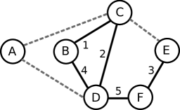
Arc	Rank
C $\to$ A	2
C $\to$ D	0
D $\to$ C	2
D $\to$ F	0
B $\to$ C	1
B $\to$ D	0

Figure 1: A $6$-node streaming graph where a batch of $5$ new edges (solid; arrival order labeled next to them) is being added to a stream of $3$ edges (dashed) that have arrived earlier—and examples of the corresponding rank values as this batch is being incoporated.

In words, if $\{x,y\}$ is an edge in $W$, $\mathop{\mathrm{rank}}(x\to y)$ is the number of edges in $W$ that are incident on $x$ and appear after $xy$ in $W$. For non-edge pairs, $\mathop{\mathrm{rank}}(x\to y)$ is simply the degree of $x$ in the graph $G_{W}$. This function is, in general, not symmetric: $\mathop{\mathrm{rank}}(x\to y)$ is not the same as $\mathop{\mathrm{rank}}(y\to x)$. We provide an example in Figure 1.

Computing rank. We give an algorithm for computing the rank of every edge, in both orientations; it outputs a sequence of length $2|W|$ in an order convenient for subsequent lookups. Following the description and proof, we show a run of the algorithm on an example graph.

Lemma 4.3.

There is a parallel algorithm ${\texttt{rankAll}}(W)$ that takes a sequence of edges $W=\langle w_{1},\dots,w_{s}\rangle$ and produces a sequence of length $2|W|$, where each entry is a record $\{{\texttt{src}},{\texttt{dst}},{\texttt{rank}},{\texttt{pos}}\}$ such that

1. $\{{\texttt{src}},{\texttt{dst}}\}=w_{i}$ for some $i=1,\dots,|W|$;

2. ${\texttt{pos}}=i$; and

3. ${\texttt{rank}}=\mathop{\mathrm{rank}}({\texttt{src}}\to{\texttt{dst}})$.

Each input edge $w_{i}$ gives rise to exactly $2$ entries, one per orientation. The algorithm runs in $O({\texttt{sort}}(s))$ cache complexity and $O(\log^{2}s)$ depth.

(Readers interested in the main idea of the algorithm may wish to skip this proof on the first read and proceed to the example in Figure 2.)

Proof.

We describe an algorithm and reason about its complexity. First, we form a sequence $F$, where each $w_{i}=\{u,v\}$ yields two records: $\{{\texttt{src}}=u,{\texttt{dst}}=v,{\texttt{pos}}=i\}$ and $\{{\texttt{src}}=v,{\texttt{dst}}=u,{\texttt{pos}}=i\}$. That is, there are two entries corresponding to each input edge, both marked with the position in the original sequence. This step can be accomplished in $O({\texttt{scan}}(s))$ cache complexity and at most $O(\log^{2}s)$ depth using map and concat.

If we view the entries of $F$ as directed edges, the rank of an arc $e\in F$, $\mathop{\mathrm{rank}}(e.{\texttt{src}}\to e.{\texttt{dst}})$, is the number of arcs in $F$ emanating from $e.{\texttt{src}}$ with ${\texttt{pos}}>e.{\texttt{pos}}$. To take advantage of this equivalent definition, we sort $F$ by src and for two entries of the same src, order them in the decreasing order of pos. This has $O({\texttt{sort}}(s))$ cost and $O(\log^{2}s)$ depth. Now, in this ordering, the rank of a particular edge is one more than the rank of the edge immediately before it unless it is the first edge of that src; the latter has rank $0$. Consequently, the rank computation for the entire sequence has cost $O({\texttt{scan}}(s))$ since all that is required is to figure out whether an edge is the first edge with that src (using combine) and a prefix scan operation (see, e.g., [13] or Appendix B). Overall, the algorithm runs in $O({\texttt{sort}}(s)+{\texttt{scan}}(s))$ cache complexity and $O(\log^{2}s)$ depth, as claimed.

rankAll$(W)=\;$

I	src:	B	B	C	C	D	D	D	E	F	F
	dst:	D	C	D	B	F	B	C	F	D	E
	pos:	4	1	2	1	5	4	2	3	5	3
II	rank:	0	1	0	1	0	1	2	0	0	1

Figure 2: Running rankAll on the example streaming graph. Each column corresponds to an entry in the output.

In Figure 2, we give an example of the output of rankAll on the example graph from Figure 1. It also illustrates the intermediate steps of the algorithm: the 3 rows marked with I show the array $F$ the algorithm has after the sort step. The line marked with II is the result after performing scan.

In addition, using this figure as an example, we make two observations about the output of rankAll that will prove useful later on.

1. it is ordered by src breaking tie in the decreasing order of pos; and

2. it is ordered by src then by rank, in the increasing order.

Mapping rank to substreams. Having defined rank and showed how to compute it, we now present an easy-to-verify observation that implicitly defines a substream with respect to a level-1 edge $f_{1}$ in terms of rank values:

Observation 4.4.

Let $f_{1}=\{u,v\}\in E\cup W$ be a level-1 edge. Let $F^{\prime}={\texttt{rankAll}}(W)$. The set of edges in $W$ incident on $f_{1}$ that appears after it—i.e., the set $\Gamma_{W}(f_{1})$—is precisely the undirected edges corresponding to $L\cup R$, where

$$L =\{e\in F^{\prime}:e.{\texttt{src}}=u,e.{\texttt{rank}}<\mathop{\mathrm{rank}}(u\to v)\}$$

and

$$R =\{e\in F^{\prime}:e.{\texttt{src}}=v,e.{\texttt{rank}}<\mathop{\mathrm{rank}}(v\to u)\}.$$

To elaborate further, we note that there are $\mathop{\mathrm{rank}}(u\to v)$ edges in $\Gamma_{W}(f_{1})$ incident on $u$ (those in $L$) and $\mathop{\mathrm{rank}}(v\to u)$ edges, on $v$ (those in $R$). As an immediate consequence, we have that $\chi^{+}=\mathop{\mathrm{rank}}(u\to v)+\mathop{\mathrm{rank}}(v\to u)$. Since $\chi^{-}$ is already known, we can readily compute the new $\chi$ value as $\chi=\chi^{+}+\chi^{-}$, as noted before.

Furthermore, we will use this as a “naming system” for identifying which level-2 edge to pick. For a level-1 edge $f_{1}$, there are $\chi^{+}$ candidates in $\Gamma_{W}(f_{1})$. We will associate each number $\phi\in\{0,1,\dots,\chi^{+}-1\}$ with an edge in $\Gamma_{W}(f_{1})$ as follows: if $\phi<\mathop{\mathrm{rank}}(u\to v)$, we associate it with the edge ${\texttt{src}}=u$ and ${\texttt{rank}}=\phi$; otherwise, associate it with the edge ${\texttt{src}}=v$ and ${\texttt{rank}}=\phi-\mathop{\mathrm{rank}}(u\to v)$. We give two examples in Figure 3 to illustrate the naming system.

$\phi$:	0	1
src:	D	D
rank:	0	1
real edge:	DF	BD

$\phi$:	0	1	2
src:	C	C	E
rank:	0	1	0
real edge:	CD	CB	EF

Figure 3: Translating rank values to substreams: (Left) $f_{1}=\textsf{\small DC}$ using $u=\textsf{\small D}$ and $v=\textsf{\small C}$, so $\chi^{+}=2$. (Right) $f_{1}=\textsf{\small CE}$ using $u=\textsf{\small C}$ and $v=\textsf{\small E}$, so $\chi^{+}=3$.

Putting them together. Armed with these ingredients, we are ready to sketch an algorithm for maintaining level-2 edges and $\chi$. We will also rely on multisearch queries of the following forms (which can be supported by Lemma 3.5)—(Q1) Given $(u,p)$, locate an edge with ${\texttt{src}}=u$ with the least pos larger or equal to $p$; and (Q2) Given $(u,a)$, locate an edge with ${\texttt{src}}=u$ with the rank exactly equal to $a$.

First, construct a length-$r$ array $\chi^{-}[]$ of $\chi^{-}$ values by copying from $\text{{est}}_{i}.\chi$ (using map). Then, for $i=1,\dots,r$, compute $\mathit{ld}[i]=\mathop{\mathrm{rank}}(u\to v)$ and $\mathit{rd}[i]=\mathop{\mathrm{rank}}(v\to u)$, where $\{u,v\}=\text{{est}}_{i}.f_{1}$; this can be done using two multisearch calls each involving $r$ queries of the form (Q1) This is sufficient information to compute the length-$r$ array $\chi^{+}[]$, where $\chi^{+}[i]=\mathit{ld}[i]+\mathit{rd}[i]$ (using combine).

Now we apply map to flip a coin for each estimator deciding whether it will take on a new level-2 edge from $W$. Using the same map operation, for every estimator $\text{{est}}_{i}$ that is replacing its level-2 edge, we pick a random number between $0$ and $\chi^{+}[i]-1$ (inclusive), which maps to an edge in the substream $\Gamma_{W}(\text{{est}}_{i}.f_{1})$ using the naming scheme above. To convert this number to an actual edge, we perform a multisearch operation involving at most $r$ queries of the form (Q2), which completes Step 2.

4.4 Step 3: Locate Closing Edges

The goal of Step 3 is to detect, for each estimator, if the wedge formed by level-1 and level-2 edges closes using a edge from $W$. For this final step, we construct a length-$|W|$ array edges, where each $w_{i}=\{u,v\}\in W$ ($u<v$) yields a record $\{{\texttt{src}}=u,{\texttt{dst}}=v,{\texttt{pos}}=i\}$. We then sort this by src, then by dst. After that, with a map operation, we compute the candidate closing edge and use a multisearch on edges with at most $r$ queries of the form “Given $(u,v)$, locate the edge $(u,v)$” This allows us to check if the candidates are present and come after the level-2 edge, by checking their pos field.

4.5 Cost Analysis

Using the terminology of Theorem 4.1, we let $s=|W|$ and $r$ be the number of estimators we maintain. Step 1 is implemented using map, extract, and combine. Therefore, the cache cost for Step 1 is at most $O({\texttt{sort}}(r)+{\texttt{scan}}(r+s))$, and the depth is at most $O(\log^{2}(r+s))$. For Step 2, the cost of running rankAll is $O({\texttt{sort}}(s))=O(\tfrac{s}{B}\log_{M/B}(1+s/B))$ memory cost and $O(\log^{2}s)$ depth. The cost of the other operations in Step 2 is dominated by $O({\texttt{sort}}(r)+{\texttt{sort}}(s))$. The total cost for Step 2 is $O({\texttt{sort}}(r)+{\texttt{sort}}(s))$ memory cost and at most $O(\log^{2}(r+s))$ depth. Likewise, in Step 2, the cost of sorting dominates the multisearch cost and map, resulting in a total cost of $O({\texttt{sort}}(r)+{\texttt{sort}}(s))$ for memory cost and at most $O(\log^{2}(r+s))$ depth.

Hence, the total cost of the bulkUpdateAll is $O({\texttt{sort}}(r)+{\texttt{sort}}(s))$ memory cost and $O(\log^{2}(r+s))$ depth, as promised.

5 Evaluation

We implemented the algorithm described in Section 4 and investigated its performance on real-world datasets in terms of accuracy, parallel speedup, parallelization overhead, effects of batch size on throughput, and cache behaviors.

Implementation. We followed the description in Section 4 rather closely. The algorithm combines the “coarse” estimators into a sharp estimate using a median-of-means aggregate. The main optimization we made was in avoiding malloc-ing small chunks of memory often. The sort primitive uses a PCO sample sort algorithm [5, 26], which offers good speedups. The multisearch routines are a modified Blelloch et al.’s merge algorithm [5]; the modification stops recursing early when the number of “queries” is small. Other primitives are standard. The main triangle counting logic has about $600$ lines of Cilk code, a dialect of C/C++ with keywords that allow users to specify what should be run in parallel [12] (fork/join-type code). Cilk’s runtime system relies on a work-stealing scheduler, a dynamic scheduler that allows tasks to be rescheduled dynamically at relatively low cost. The scheduler is known to impose only little overhead on both parallel and sequential code. Our benchmark programs were compiled with the public version of Cilk shipped with GNU g++ Compiler version 4.8.0 (20130109). We used the optimization flag -O2.

Testbed and Datasets. We performed experiments on a $12$-core (with hyperthreading) Intel machine, running Linux 2.6.32-279 (CentOS 6.3). The machine has two $2.67$ Ghz $6$-core Xeon X5650 processors with $96$GB of memory although the experiments never need more a few gigabytes of memory.

Our study uses a collection of graphs, obtained from the SNAP project at Stanford [21] and a recent Twitter dataset [16]. We present a summary of these datasets in Table 1. We simulate a streaming graph by feeding the algorithm with edges as they are read from disk. As we note later on, disk I/O is not a bottleneck in the experiment.

With the growth of social media in recent years, some of the biggest graphs to date arise in this context. When we went looking for big graphs to experiment with, most graphs that turned up happen to stem from this domain. While this means we experimented with the graphs that triangle counting is likely used for, we will note that our algorithm does not assume any special property about it.

Dataset	$n$	$m$	$\Delta$	$\tau$	$m\Delta/\tau$	Size
Amazon	334,863	925,872	1,098	667,129	1,523.85	13M
DBLP	317,080	1,049,866	686	2,224,385	323.78	14M
LiveJournal	3,997,962	34,681,189	29,630	177,820,130	5,778.89	0.5G
Orkut	3,072,441	117,185,083	66,626	627,584,181	12,440.68	1.7G
Friendster	65,608,366	1,806,067,135	5,214	4,173,724,142	2,256.22	31G
Powerlaw (synthetic)	267,266,082	9,326,785,184	6,366,528	-	-	167GB

Table 1: A summary of the datasets used in our experiments, showing for every dataset, the number of nodes ($n$), the number of edges ($m$), the maximum degree ($\Delta$), the number of triangles in the graph ($\tau$), the ratio $m\Delta/\tau$, and size on disk (stored as a list of edges in plain text).

For most datasets, the exact triangle count is provided by the source (which we have verified); in other cases, we compute the exact count using an algorithm developed as part of the Problem-Based Benchmark Suite [26]. We also report the size on disk of these datasets in the format we obtain them (a list of edges in plain text). In addition, we include one synthetic power-law graph; on this graph, we cannot obtain the true count, but it is added to speed test the algorithm.

Baseline. For accuracy study, we directly compare our results with the true count. For performance study, our baseline is a fairly optimized version of the nearly-linear time algorithm based on neighborhood sampling, using bulk-update, as described in [25]. We use this baseline to establish the overhead of the parallel algorithm. We do not compare the accuracy between the two algorithms because by design, they produce the exact same answer given the same sequence of random bits. The baseline code was also compiled with g++ version 4.8.0 but without linking with the Cilk runtime.

5.1 Performance and Accuracy

We perform experiments on graphs with varying sizes and densities. Our algorithm is randomized and may behave differently on different runs. For robustness, we perform five trials—except when running the biggest datasets on a single core, where only two trials are used. Table 5.1 shows for different numbers of estimators $r=200\text{K},2\text{M},20\text{M}$, the accuracy, reported as the mean deviation value, and processing times (excluding I/O) using $1$ and all $12$ cores (24 threads with hyperthreading), as well as the speedup ratio. Mean deviation is a well-accepted measure of error, which, we believe, accurately depicts how well the algorithm performs. In addition, it reports the median I/O time In another experiment, presented in Table 5.1, we compare our parallel implementation with the baseline sequential implementation [25]. As is evident from the findings, the I/O cost is not a bottleneck in any of the experiments, justifying the need for parallelism to improve throughput.

Dataset	$r=200$K					$r=2$M					$r=20$M				I/O
	MD	$T_{1}$	$T_{12H}$	$\frac{T_{1}}{T_{12H}}$		MD	$T_{1}$	$T_{12H}$	$\frac{T_{1}}{T_{12H}}$		MD	$T_{1}$	$T_{12H}$	$\frac{T_{1}}{T_{12H}}$
Amazon	$2.08$	$1.07$	$0.14$	$7.64$		$0.47$	$3.58$	$0.42$	$8.52$		$0.12$	$29.00$	$3.15$	$9.21$	0.14
DBLP	$1.18$	$1.21$	$0.17$	$7.12$		$0.39$	$3.71$	$0.43$	$8.63$		$0.08$	$29.20$	$3.14$	$9.30$	0.15
LiveJournal	$5.51$	$35.10$	$3.31$	$10.60$		$0.51$	$41.00$	$3.91$	$10.49$		$0.39$	$69.80$	$6.56$	$10.64$	1.52
Orkut	$2.39$	$119.00$	$11.20$	$10.62$		$0.16$	$133.00$	$12.40$	$10.73$		$0.66$	$172.00$	$15.40$	$11.17$	5.00
Friendster	$18.25$	$1730.00$	$181.00$	$9.56$		$8.35$	$1970.00$	$193.00$	$10.21$		$3.41$	$2330.00$	$219.00$	$10.64$	86.00

Powerlaw $-$ $-$ $-$ $-$ $-$ $-$ $-$ $-$ $-$ $-$ $1050.0$ $-$ $970.00$

Table 2: The accuracy (MD is mean deviation, in percentage), median processing time on $1$ core $T_{1}$ (in seconds), median processing time on $12$ cores $T_{12H}$ with hyperthreading (in seconds), and I/O time (in seconds) of our parallel algorithm across five runs as the number of estimators $r$ is varied.

Several trends are evident from these experiments. First, the algorithm is accurate with only a modest number of estimators. In all datasets, including the one with more than a billion edges, the algorithm achieves less than $4$% mean deviation using about $20$ million estimators, and for smaller datasets, it can obtain better than $5$% mean deviation using fewer estimators. As a general trend—though not a strict pattern—the accuracy improves with the number of estimators. Furthermore, in practice, far fewer estimators than suggested by the pessimistic theoretical bound is necessary to reach a desired accuracy. For example, on Twitter-2010, which has the highest $m\Delta/\tau$ ratio among the datasets, using $\varepsilon=0.0386$, the expression $96/\varepsilon^{2}\cdot m\Delta/\tau$ (see Theorem 3.4) is at least $6.6$ billion, but we reach this accuracy using $20$ million estimators.

Second, the algorithm shows substantial speedups on all datasets. On all datasets, the experiments show that the algorithm achieves up to $11.24$x speedup on $12$ cores, with the speedup numbers ranging between $7.5$x and $11.24$x. On the biggest datasets using $r=20\text{M}$ estimators, the speedups are consistently above $10$x. This shows that the algorithm is able to effectively utilize available cores except when the dataset or the number of estimators is too small to fully utilize parallelism. Additionally, we experimented with a big synthetic graph (167GB power-law graph) to get a sense of the running time. For this dataset, we were unable to calculate the true count; we also cut short the sequential experiment after a few hours. But it is worth pointing out that this dataset has $5$x more edges than Friendster, and our algorithm running on 12 cores finishes in $1050$ seconds (excluding I/O)—about $5$x longer than on Friendster.

Table 3: The median processing time of the sequential algorithm $T_{\text{seq}}$ (in seconds), the median processing time of the parallel algorithm running on $1$ core $T_{1}$ (in seconds), and the overhead factor (i.e., $T_{1}/T_{\text{seq}}$).

Third, the overhead is well-controlled. Both the sequential and parallel algorithms, at the core, maintain the same neighborhood sampling invariant but differ significantly in how the edges are processed. As is apparent from Table 5.1, for large datasets requiring more estimators, the overhead is less than $1.5$x with $r=20\text{M}$. For smaller datasets, the overhead is less than $1.6$x with $r=2\text{M}$. In all cases, the amount of speedup gained outweighs the overhead.

5.2 Additional Experiments

The previous set of experiments studies the accuracy, scalability, and overhead of our parallel algorithm, showing that it scales well and has low overhead. We report on another set of experiments designed to help understand the algorithm’s behaviors in more detail.

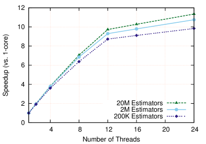
Figure 4: Speedup on the Friendster dataset as the number of cores and the number of estimators are varied.

Scalability. To further our understanding of the algorithm’s scalability, we take the biggest real dataset (Friendster) and examine its speedup behavior as the number of threads is varied. Figure 4 shows, for $r=200\mbox{K},2\mbox{M},20\mbox{M}$, the speedup ratio with respect to the parallel code running on $1$ core. On a $12$-core machine, the speedup grows linearly with the number of threads until $12$ threads (the number of physical cores); the growth slows down after that but keeps rising until $24$ threads since we are now running on hyperthreaded cores. The trend seems invariable with the number of estimators $r$ although the speedup ratio improves with larger $r$ since there is more work for parallelism.

As a next step, we attempt to understand how the speedup is gained and how it is likely to scale in the future on other machines. For this, we examine the breakdown of how the time is spent in different components of the algorithm. Figure 5 shows the fractions of time spent inside sort, multisearch routines, and other components for the $3$ biggest datasets. The figure shows that the majority of the time is spent on sorting (up to $94\%$), which has great speedups in our setting. The multisearch portion makes up less than $5\%$ of the running time. The remaining $1\%$ is spent in miscellaneous bookkeeping. Because we can directly use an off-the-shelf sorting implementation, this main portion will improve with the performance of sort. We expect the algorithm to continue to scale well on machines with more cores, as cache-efficient sort has been shown to scale [26].

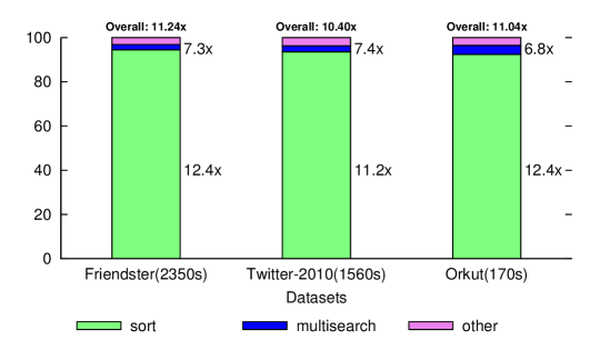
Figure 5: The timing breakdown (in percentage of time) of the parallel algorithm on the $3$ largest datasets running on $1$ core. The number in parenthesis next to each dataset is the $T_{1}$ (in seconds) whereas the numbers next to the columns are the speedup ratio for the corresponding components running with 24 threads (all 12 cores with hyperthreading).

Batch Size vs. Throughput. How does the choice of a batch size affect the overall performance of our algorithm? We study this question empirically by measuring the sustained throughput as the batch size is varied. Figure 6 shows the results on the dataset Orkut running with $r=2\mbox{M}$ and $24$ threads. Orkut was chosen so that we understand the performance trend on medium-sized graphs, showing that our scheme can benefit not only the largest graphs but also smaller ones. We expect intuitively that the throughput improves with the batch size, and the experiment confirms that, reaching about $9.3$ million edges per second using a batch size of $16\mbox{M}$.

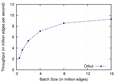
Figure 6: The sustained throughput the algorithm with varying batch sizes on the graph Orkut using $r=2\mbox{M}$ and $24$ threads.

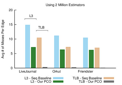
Figure 7: The average number of L3 cache misses per edge and the average number of TLB misses per edge as reported by perftool on representative datasets running with $r=2$M estimators. Both algorithms were run single-threaded.

Cache Behavior. We also study the memory access cost of the parallel cache-oblivious algorithm compared to the sequential baseline, which uses hash tables and performs a number of random accesses. Both algorithms were run on a single core with the same number of estimators (hence roughly the same memory footprint). For this study, we consider the number of L3 misses and TLB (Translation Lookaside Buffer) misses. Misses in these places are expensive, exactly what a cache-efficient algorithm tries to minimize. In Figure 7, we show the numbers of L3 and TLB misses normalized by the number of edges processed; the normalization helps compares results from datasets of different sizes. From this figure, it is clear that our cache-efficient scheme has significantly lower cache/TLB misses.

6 Conclusion

We have presented a cache-efficient parallel algorithm for approximating the number of triangles in a massive streaming graph. The proposed algorithm is cache-oblivious and has good theoretical performance and accuracy guarantees. We also experimentally showed that the algorithm is fast and accurate, and has low cache complexity. It will be interesting to explore other problems at the intersection of streaming algorithms and parallel processing.

Acknowledgments

Tangwongsan was in part sponsored by the U.S. Defense Advanced Research Projects Agency (DARPA) under the Social Media in Strategic Communication (SMISC) program, Agreement Number W911NF-12-C-0028. The views and conclusions contained in this document are those of the author(s) and should not be interpreted as representing the official policies, either expressed or implied, of the U.S. Defense Advanced Research Projects Agency or the U.S. Government. The U.S. Government is authorized to reproduce and distribute reprints for Government purposes notwithstanding any copyright notation hereon. Pavan was sponsored in part by NSF grant 0916797; Tirthapura was sponsored in part by NSF grants 0834743 and 0831903.

Appendix A More Detailed Models

Parallel algorithms in this work are expressed in the nested parallel model. It allows arbitrary dynamic nesting of parallel loops and fork-join constructs but no other synchronizations, corresponding to the class of algorithms with series-parallel dependency graphs. In this model, computations can be recursively decomposed into tasks, parallel blocks, and strands, where the top-level computation is always a task:

• The smallest unit is a strand s, a serial sequence of instructions not containing any parallel constructs or subtasks.

• A task t is formed by serially composing $k\geq 1$ strands interleaved with $k-1$ parallel blocks, denoted by $\texttt{t}=\texttt{s}_{1};\texttt{b}_{1};\dots;\texttt{s}_{k}$.

• A parallel block b is formed by composing in parallel one or more tasks with a fork point before all of them and a join point after, denoted by $\texttt{b}=\texttt{t}_{1}\|\texttt{t}_{2}\|\dots\|\texttt{t}_{k}$. A parallel block can be, for example, a parallel loop or some constant number of recursive calls.

The depth (aka. span) of a computation is the length of the longest path in the dependence graph.

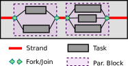
Figure 8: Expressing a computation as tasks, strands and parallel blocks

We analyze memory-access cost of parallel algorithms in the Parallel Cache Oblvivious (PCO) model [2], a parallel variant of the cache oblivious (CO) model. The Cache Oblivious (CO) model [11] is a model for measuring cache misses of an algorithm when run on a single processor machine with a two-level memory hierarchy—one level of finite cache and unbounded memory. The cache complexity measure of an algorithm under this model $Q\left({n;M{},B{}}\right)$ counts the number of cache misses incurred by a problem instance of size $n$ when run on a fully associative cache of size $M{}$ and line size $B{}$ using the optimal (offline) cache replacement policy.

Extending the CO model, the PCO model gives a way to analyze the number of cache misses for the tasks that run in parallel in a parallel block. The PCO model approaches it by (i) ignoring any data reuse among the parallel subtasks and (ii) assuming the cache is flushed at each fork and join point of any task that does not fit within the cache.

More precisely, let $\textit{loc}(\texttt{t}{};B{})$ denote the set of distinct cache lines accessed by task t, and $S(\texttt{t}{};B{})=|\textit{loc}(\texttt{t}{};B{})|\cdot B{}$ denote its size. Also, let $s(\texttt{t};B)=|\textit{loc}(\texttt{t};B)|$ denote the size in terms of number of cache lines. Let $Q(\texttt{c}{};M{},B{};\kappa)$ be the cache complexity of c in the sequential CO model when starting with cache state $\kappa$.

Definition A.1 (Parallel Cache-Oblivious Model).

For cache parameters $M$ and $B$ the cache complexity of a strand, parallel block, and a task starting in cache state $\kappa$ are defined recursively as follows (see [2] for detail).

$Q^{*}(\texttt{t}{};M{},B{};\kappa)$ $=\sum_{i=1}^{k}Q^{*}(\texttt{c}_{i};M{},B{};\kappa_{i-1})$, where $\kappa_{i}=\emptyset$ if $S(\texttt{t};B)>M$, and $\kappa_{i}=\kappa\cup_{j=1}^{i}\textit{loc}(\texttt{c}_{j};B)$ if $S(\texttt{t};B)\leq M$.

We use $Q^{*}(\texttt{c}{};M{},B{})$ to denote a computation c starting with an empty cache and overloading notation, we write $Q^{*}(n;M{},B{})$ when $n$ is a parameter of the computation. We note that $Q^{*}(\texttt{c}{};M{},B{})\geq Q(\texttt{c}{};M{},B{})$. That is, the PCO gives cache complexity costs that are always at least as large as the CO model. Therefore, any upper bound on the PCO is an upper bound on the CO model. Finally, when applied to a parallel machine, $Q^{*}$ is a “work-like” measure and represents the total number of cache misses across all processors. An appropriate scheduler is used to evenly balance them across the processors.

Appendix B Scan With Resets

The following technique is standard (see, e.g., [13]); we only present it here for reference. We describe how to implement a parallel prefix sum operation with reset (also known as segmented scan), where the input is a sequence $A$ such that $A_{i}\in\{\textsf{1},\emptyset\}$. Sequentially, the desired output can computed by the following code:

sum = 0
for i = 1 to |A| do
	out[i] = sum
	if (A[i] == $\emptyset$) sum = 0 else sum += A[i]
end

That is, we keep a accumulator which is incremented every time a 1 is encountered and reset back to $0$ upon encountering $\emptyset$. This process is easy to parallelize using scan with a binary associative operator such as the following. Let $\oplus:D\times D\to D$, where $D={\mathbb{Z}}\cup\{\emptyset\}$, be given by

$$\oplus(x,y)=\begin{cases}x+y&\text{ if }x\neq\emptyset\text{ and }y\neq\emptyset\\ y&\text{ if }y\neq\emptyset\\ 0&\text{ otherwise }\end{cases}$$

References

- BBCG [08] L. Becchetti, P. Boldi, C. Castillo, and A. Gionis. Efficient semi-streaming algorithms for local triangle counting in massive graphs. In Proc. ACM Conference on Knowledge Discovery and Data Mining (KDD), pages 16–24, 2008.
- BFGS [11] Guy E. Blelloch, Jeremy T. Fineman, Phillip B. Gibbons, and Harsha Vardhan Simhadri. Scheduling irregular parallel computations on hierarchical caches. In SPAA’11, pages 355–366, New York, NY, USA, 2011. ACM.
- BFLS [07] Luciana S. Buriol, Gereon Frahling, Stefano Leonardi, and Christian Sohler. Estimating clustering indexes in data streams. In Proc. European Symposium on Algorithms (ESA), pages 618–632, 2007.
- BFN+ [11] J. W. Berry, L. Fosvedt, D. Nordman, C. A. Phillips, and A. G. Wilson. Listing triangles in expected linear time on power law graphs with exponent at least 7/3. Technical report, Sandia National Laboratories, 2011.
- BGS [10] Guy E. Blelloch, Phillip B. Gibbons, and Harsha Vardhan Simhadri. Low depth cache-oblivious algorithms. In SPAA’10, pages 189–199, New York, NY, USA, 2010. ACM.
- BYKS [02] Ziv Bar-Yossef, Ravi Kumar, and D. Sivakumar. Reductions in streaming algorithms, with an application to counting triangles in graphs. In Proc. ACM-SIAM Symposium on Discrete Algorithms (SODA), pages 623–632, 2002.
- CC [11] S. Chu and J. Cheng. Triangle listing in massive networks and its applications. In Knowledge Data and Discovery (KDD), pages 672–680, 2011.
- CN [85] N. Chiba and T. Nishizeki. Arboricity and subgraph listing algorithms. SIAM Journal on computing, 14:210–223, 1985.
- Coh [09] J. Cohen. Graph twiddling in a mapreduce world. Computing in Science and Engineering, 11:29–41, 2009.
- EM [02] Jean-Pierre Eckmann and Elisha Moses. Curvature of co-links uncovers hidden thematic layers in the world wide web. Proceedings of the National Academy of Sciences, 99(9):5825–5829, 2002.
- FLPR [99] Matteo Frigo, Charles E. Leiserson, Harald Prokop, and Sridhar Ramachandran. Cache-oblivious algorithms. In FOCS, 1999.
- Int [13] Intel Cilk Plus, 2013. http://cilkplus.org/.
- JáJ [92] Joseph JáJá. An Introduction to Parallel Algorithms. Addison-Wesley, 1992.
- JG [05] Hossein Jowhari and Mohammad Ghodsi. New streaming algorithms for counting triangles in graphs. In Proc. 11th Annual International Conference Computing and Combinatorics (COCOON), pages 710–716, 2005.
- JSP [12] Madhav Jha, C. Seshadhri, and Ali Pinar. From the birthday paradox to a practical sublinear space streaming algorithm for triangle counting. CoRR, abs/1212.2264, 2012.
- KLPM [10] Haewoon Kwak, Changhyun Lee, Hosung Park, and Sue B. Moon. What is Twitter, a social network or a news media? In WWW, pages 591–600, 2010.
- KMPT [10] Mihail N. Kolountzakis, Gary L. Miller, Richard Peng, and Charalampos E. Tsourakakis. Efficient triangle counting in large graphs via degree-based vertex partitioning. In WAW, pages 15–24, 2010.
- KMSS [12] Daniel M. Kane, Kurt Mehlhorn, Thomas Sauerwald, and He Sun. Counting arbitrary subgraphs in data streams. In Proc. International Colloquium on Automata, Languages, and Programming (ICALP), pages 598–609, 2012.
- KP [13] Konstantin Kutzkov and Rasmus Pagh. On the streaming complexity of computing local clustering coefficients. In Proceedings of 6th ACM conference on Web Search and Data Mining (WSDM), 2013.
- Lat [08] M. Latapy. Main-memory triangle computations for very large (sparse (power-law)) graphs. Theoretical Computer Science, 407:458–473, 2008.
- Les [12] Jure Leskovec. Stanford large network dataset collection. http://snap.stanford.edu/data/index.html, 2012. Accessed Dec 5, 2012.
- MMPS [11] Madhusudan Manjunath, Kurt Mehlhorn, Konstantinos Panagiotou, and He Sun. Approximate counting of cycles in streams. In Proc. European Symposium on Algorithms (ESA), pages 677–688, 2011.
- New [03] M. E. J. Newman. The structure and function of complex networks. SIAM REVIEW, 45:167–256, 2003.
- PT [12] Rasmus Pagh and Charalampos E. Tsourakakis. Colorful triangle counting and a mapreduce implementation. Inf. Process. Lett., 112(7):277–281, 2012.
- PTTW [13] A. Pavan, Kanat Tangwongsan, Srikanta Tirthapura, and Kun-Lung Wu. Counting and sampling triangles from a graph stream. PVLDB, 6(14), 2013.
- SBF+ [12] Julian Shun, Guy E. Blelloch, Jeremy T. Fineman, Phillip B. Gibbons, Aapo Kyrola, Harsha Vardhan Simhadri, and Kanat Tangwongsan. Brief announcement: the problem based benchmark suite. In Proc. ACM Symposium on Parallelism in Algorithms and Architectures (SPAA), pages 68–70, 2012.
- SV [11] Siddharth Suri and Sergei Vassilvitskii. Counting triangles and the curse of the last reducer. In Proc. 20th International Conference on World Wide Web (WWW), pages 607–614, 2011.
- SW [05] Thomas Schank and Dorothea Wagner. Finding, counting and listing all triangles in large graphs, an experimental study. In Workshop on Experimental and Efficient Algorithms (WEA), pages 606–609, 2005.
- TDM+ [11] Charalampos E. Tsourakakis, Petros Drineas, Eirinaios Michelakis, Ioannis Koutis, and Christos Faloutsos. Spectral counting of triangles via element-wise sparsification and triangle-based link recommendation. Social Netw. Analys. Mining, 1(2):75–81, 2011.
- TKMF [09] Charalampos E. Tsourakakis, U. Kang, Gary L. Miller, and Christos Faloutsos. Doulion: counting triangles in massive graphs with a coin. In Proc. ACM SIGKDD International Conference on Knowledge Discovery and Data Mining (KDD), pages 837–846, 2009.
- WF [94] S. Wasserman and K. Faust. Social Network Analysis. Cambridage University Press, 1994.