Fractional Klein–Gordon equations and related stochastic processes

Abstract.

This paper presents finite-velocity random motions driven by fractional Klein–Gordon equations of order $\alpha\in(0,1]$. A key tool in the analysis is played by the McBride’s theory which converts fractional hyper-Bessel operators into Erdélyi–Kober integral operators.

Special attention is payed to the fractional telegraph process whose space-dependent distribution solves a non-homogeneous fractional Klein–Gordon equation. The distribution of the fractional telegraph process for $\alpha=1$ coincides with that of the classical telegraph process and its driving equation converts into the homogeneous Klein–Gordon equation.

Fractional planar random motions at finite velocity are also investigated, the corresponding distributions obtained as well as the explicit form of the governing equations. Fractionality is reflected into the underlying random motion because in each time interval a binomial number of deviations $B(n,\alpha)$ (with uniformly-distributed orientation) are considered. The parameter $n$ of $B(n,\alpha)$ is itself a random variable with fractional Poisson distribution, so that fractionality acts as a subsampling of the changes of direction. Finally the behaviour of each coordinate of the planar motion is examined and the corresponding densities obtained.

Extensions to $N$-dimensional fractional random flights are envisaged as well as the fractional counterpart of the Euler–Poisson–Darboux equation to which our theory applies.

1. Introduction

In this paper we consider Klein–Gordon type fractional equations of the form

(1.1) $$\left(\frac{\partial^{2}}{\partial t^{2}}-c^{2}\frac{\partial^{2}}{\partial x^{2}}\right)^{\alpha}u(x,t)=\lambda^{2}u(x,t),\qquad\alpha\in(0,1].$$

The equation (1.1) in a natural way emerges within the framework of relativistic quantum mechanics for $\lambda^{2}<0$ from the expression of relativistic energy (Sakurai, 1967). Hereafter we simply call (1.1) fractional Klein–Gordon equation, for any $\lambda\in\mathbb{R}$. By means of the transformation

$$w=\sqrt{c^{2}t^{2}-x^{2}},$$

equation (1.1) takes the form

(1.2) $$\left(\frac{d^{2}}{dw^{2}}+\frac{1}{w}\frac{d}{dw}\right)^{\alpha}u(w)=\frac{\lambda^{2}}{c^{2\alpha}}u(w),$$

where a fractional power of the Bessel operator

(1.3) $$L_{B}=\frac{d^{2}}{dw^{2}}+\frac{1}{w}\frac{d}{dw}=\frac{1}{w^{2}}\left(w\frac{d}{dw}w\frac{d}{dw}\right)$$

appears. The fractional Bessel operator $(L_{B})^{\alpha}$ can be studied by means of the McBride approach to the fractional calculus (McBride, 1982, 1975, 1979). In particular,

$$(L_{B})^{\alpha}f(w) =\left(\frac{d^{2}}{dw^{2}}+\frac{1}{w}\frac{d}{dw}\right)^{\alpha}f(w)=4^{\alpha}w^{-2\alpha}I_{2}^{0,-\alpha}I_{2}^{0,-\alpha}f(w),$$

where the integral operators $I_{2}^{0,-\alpha}$ are special cases of the Erdélyi–Kober fractional integrals (see McBride, 1982, formula (2.10))

(1.4) $$I_{m}^{\eta,\alpha}f=\frac{x^{-m\eta-m\alpha}}{\Gamma(\alpha)}\int_{0}^{x}(x^{m}-u^{m})^{\alpha-1}u^{m\eta}f(u)\,d(u^{m}),$$

for $\alpha>0$ and $f$ belonging to a suitable functional space (see Section 2).

The telegraph equation (equation of damped vibrations of strings)

(1.5) $$\frac{\partial^{2}u}{\partial t^{2}}+2\lambda\frac{\partial u}{\partial t}=c^{2}\frac{\partial^{2}u}{\partial x^{2}}$$

can be reduced to the classical Klein–Gordon equation ((1.1) with $\alpha=1$) by means of the transformation $u(x,t)=e^{-\lambda t}v(x,t)$. Equation (1.5) governs the distribution of the telegraph process $\mathcal{T}(t)$, $t\geq 0$, and the related Klein–Gordon equation directs the absolutely continuous component of the distribution of $\mathcal{T}(t)$ (see, for example, De Gregorio et al. (2005)). The telegraph process is a finite-velocity one-dimensional random motion of which many probabilistic features are well known. In this paper we study fractional extensions of the telegraph process, denoted by $\mathcal{T}^{\alpha}(t)$, $t\geq 0$, whose changes of direction are somehow related to the fractional Poisson process $\mathcal{N}^{\alpha}(t)$, $t\geq 0$, with one-dimensional distribution given by (Beghin and Orsingher, 2009)

(1.6) $$P\{\mathcal{N}^{\alpha}(t)=k\}=\frac{1}{E_{\alpha,1}(\lambda t^{\alpha})}\frac{\left(\lambda t^{\alpha}\right)^{k}}{\Gamma(\alpha k+1)},\qquad\alpha\in(0,1],\>k=0,1,\dots,$$

with

(1.7) $$E_{\alpha,1}(\lambda t^{\alpha})=\sum_{k=0}^{\infty}\frac{(\lambda t^{\alpha})^{k}}{\Gamma(\alpha k+1)}.$$

The probability law of $\mathcal{T}^{\alpha}(t)$, $t\geq 0$, can be written as

(1.8) $$p^{\alpha}(x,t)={} \frac{1}{E_{\alpha,1}(\lambda t^{\alpha})}\bigg{[}ct\sum_{k=1}^{\infty}\left(\frac{\lambda}{2^{\alpha}c^{\alpha}}\right)^{2k}\frac{(c^{2}t^{2}-x^{2})^{\alpha k-1}}{\Gamma(\alpha k)\Gamma(\alpha k+1)}+\sum_{k=0}^{\infty}\left(\frac{\lambda}{2^{\alpha}c^{\alpha}}\right)^{2k+1}\frac{(c^{2}t^{2}-x^{2})^{\alpha k+\frac{\alpha-1}{2}}}{[\Gamma(\alpha k+\frac{1+\alpha}{2})]^{2}}\bigg{]}$$

$$+\frac{1}{2E_{\alpha,1}(\lambda t^{\alpha})}[\delta(x+ct)+\delta(x-ct)],\qquad\alpha\in(0,1],\;\mbox{for $|x|\leq ct$}.$$

In (1.8), multi-index Mittag–Leffler functions (Kiryakova, 2000) of the form

(1.9) $$E^{(2)}_{(\alpha_{j}),(\beta_{j})}(x)=\sum_{k=0}^{\infty}\frac{x^{k}}{\prod_{j=1}^{2}\Gamma(\beta_{j}+k\alpha_{j})}$$

appear. We note that, for $\alpha_{j}=\beta_{j}=1$, the multi-index Mittag–Leffler function (1.9) coincides with the modified Bessel function of the second order.

The conditional distributions $P\{\mathcal{T}^{\alpha}(t)\in dx|\mathcal{N}^{\alpha}(t)=n\}$, in analogy to the conditional laws of the telegraph process $\mathcal{T}(t)$ can be obtained by means of the order statistics (see De Gregorio et al., 2005). The fractional telegraph-type process can thus be regarded as a continuous-time random motion with a rightward step (up to a Beta-distributed instant) and a leftward motion during the subsequent time span.

We consider also the multidimensional Klein–Gordon-type fractional equation

(1.10) $$\left(\frac{\partial^{2}}{\partial t^{2}}-c^{2}\Delta\right)^{\alpha}u(\mathbf{x},t)=\lambda^{2}u(\mathbf{x},t),\qquad\mathbf{x}\in\mathbb{R}^{N},\>t\geq 0,0<\alpha\leq 1,$$

and a particular attention is devoted to the planar case ($N=2$). For $N=2$ and $\alpha=1$, equation (1.10) can be obtained by means of the exponential transformation

$$v(x,y,t)=e^{-\lambda t}u(x,y,t),$$

from the planar telegraph equation (also called equation of planar vibrations with damping)

(1.11) $$\frac{\partial^{2}v}{\partial t^{2}}+2\lambda\frac{\partial v}{\partial t}=c^{2}\left(\frac{\partial^{2}}{\partial x^{2}}+\frac{\partial^{2}}{\partial y^{2}}\right)v,$$

which governs the distribution of a planar random motion with infinite directions (see Kolesnik and Orsingher, 2005). A time-fractional telegraph equation was examined in Orsingher and Beghin (2004) and the related composition of the telegraph process with a reflecting Brownian motion analyzed for $\alpha=\frac{1}{2}$. Recently more general space-time fractional telegraph equations in $\mathbb{R}^{N}$ were investigated in Orsingher and Toaldo (2013) and their solutions derived as the distribution of a composition of stable processes at the inverse of linear combinations of stable subordinators. We are able to obtain a fractional planar random motion $(X^{\alpha}(t),Y^{\alpha}(t))$, $t\geq 0$, which generalizes that treated in Kolesnik and Orsingher (2005) and has explicit distribution

(1.12) $$P\{X^{\alpha}(t)\in dx,Y^{\alpha}(t)\in dy\} =\frac{dx\,dy\,\lambda}{2\pi c^{\alpha}E_{\alpha,1}(\lambda t^{\alpha})}\frac{E_{\alpha,\alpha}\left(\frac{\lambda}{c^{\alpha}}\left(\sqrt{c^{2}t^{2}-(x^{2}+y^{2})}\right)^{\alpha}\right)}{\left(\sqrt{c^{2}t^{2}-(x^{2}+y^{2})}\right)^{2-\alpha}}$$

$$=\frac{dx\,dy\,\lambda\,u_{\alpha}(x,y,t)}{2\pi c^{\alpha}E_{\alpha,1}(\lambda t^{\alpha})},\qquad(x,y)\in C_{ct},$$

where

$$C_{ct}=\{(x,y)\in\mathbb{R}^{2}:x^{2}+y^{2}\leq c^{2}t^{2}\}.$$

The function $u_{\alpha}$ appearing in (1.12) is a solution to the non-homogeneous fractional Klein–Gordon equation

$$\left(\frac{\partial^{2}}{\partial t^{2}}-c^{2}\left\{\frac{\partial^{2}}{\partial x^{2}}+\frac{\partial^{2}}{\partial y^{2}}\right\}\right)^{\alpha}u_{\alpha}(x,y,t)=\lambda^{2}u_{\alpha}(x,y,t)+\frac{\lambda c^{\alpha}}{\Gamma(-\alpha)}\left(\sqrt{c^{2}t^{2}-x^{2}-y^{2}}\right)^{-\alpha-2},$$

which reduces to a homogeneous one in the classical case $\alpha=1$. The random motions worked out in this paper develop at finite velocity and the support of their distributions is a compact set. For this reason the fractional models dealt with here substantially differ from those appeared so far in the literature (Orsingher and Beghin, 2004). The fractional planar random motion considered here can be described by a particle where the number of changes of direction coincides with a fraction $\alpha$ of the changes of direction of orientation of the classical model.

The projection of the fractional planar motion $(X^{\alpha}(t),Y^{\alpha}(t))$ on the $x$-axis has probability density

(1.13) $$p_{\alpha}(x,t)=\frac{1}{E_{\alpha,1}(\lambda t^{\alpha})}\frac{\lambda}{2^{\alpha}c^{\alpha}}\sum_{k=0}^{\infty}\left(\frac{\lambda}{2^{\alpha}c^{\alpha}}\right)^{k}\frac{\left(\sqrt{c^{2}t^{2}-x^{2}}\right)^{k\alpha-1}}{[\Gamma(\frac{\alpha k+1}{2})]^{2}},\qquad x\in[-ct,+ct].$$

Therefore the distribution $p_{\alpha}(x,t)$ does not possess singular components as its planar counterpart (as well as the one-dimensional fractional telegraph process). If $\alpha=1$, we retrieve the distribution (1.3) of Orsingher and De Gregorio (2007) which is expressed in terms of Struve functions.

A solution of the $N$-dimensional fractional Klein–Gordon equation has been obtained in the form

(1.14) $$u_{\alpha}(\mathbf{x},t)=\sum_{k=0}^{\infty}\left(\frac{\lambda}{2^{\alpha}c^{\alpha}}\right)^{2k}\frac{\left(\sqrt{c^{2}t^{2}-\sum_{j=1}^{N}x_{j}^{2}}\right)^{2\alpha k+2\alpha-2}}{\Gamma(\alpha k+\alpha+\frac{N-1}{2})\Gamma(\alpha k+\alpha)},\qquad\sum_{j=1}^{N}x_{j}^{2}\leq c^{2}t^{2}.$$

From (1.14), the following conditional distribution can be extracted.

(1.15) $$P\{X_{1}(t)\in dx_{1},\dots,X_{N}(t)\in dx_{N}|\mathcal{N}^{\alpha}(t)=k\}=\frac{\Gamma(\frac{k\alpha+N}{2})\left(\sqrt{c^{2}t^{2}-\|x_{n}\|^{2}}\right)^{\alpha k-2}}{(ct)^{\alpha k+N-2}\Gamma(\frac{\alpha k}{2})\pi^{N/2}}.$$

If $N=2$ the density (1.15) coincides with the conditional distribution of $(X^{\alpha}(t),Y^{\alpha}(t))$, and for $\alpha=1$, we recover result (5) of Kolesnik and Orsingher (2005). For $N=4$, $\alpha=2$ we extract from (1.15) the distribution (3.2) of Orsingher and De Gregorio (2007). An extension of this theory for $\alpha>1$ is considered below.

The last section of this paper is devoted to higher-order fractional Bessel-type equations of the form

(1.16) $$\Biggl{(}\frac{1}{w^{n}}\Biggl{(}\underbrace{w\frac{d}{dw}w\frac{d}{dw}\dots w\frac{d}{dw}}_{\text{$n$ derivatives}}\Biggr{)}\Biggr{)}^{\alpha}f(w)=\lambda^{n}f(w).$$

These higher-order Bessel equations arise within the framework of cyclic motions in $\mathbb{R}^{N}$ with the minimal number $N+1$ of velocities directed on the edges of a hyperpolyhedron (see for example Lachal et al., 2006). A special attention is devoted to the case of three orthogonal directions, where the distribution of $(X(t),Y(t))$, for $\alpha=1$ can be expressed in terms of third-order Bessel functions

$$I_{0,3}(x)=\sum_{k=0}^{\infty}\left(\frac{x}{3}\right)^{3k}\frac{1}{(k!)^{3}}.$$

An application of the McBride theory of fractional powers of differential operators to the Euler–Poisson–Darboux fractional equations is also considered.

2. Preliminaries on fractional hyper-Bessel operators

Our starting point is the generalized hyper-Bessel operator, considered in McBride (1982),

(2.1) $$L=x^{a_{1}}Dx^{a_{2}}\dots x^{a_{n}}Dx^{a_{n+1}},$$

where $n$ is an integer number, $a_{1},\dots,a_{n+1}$ are complex numbers and $D=d/dx$. Hereafter we assume that the coefficients $a_{j}$, $j=1,\dots,n+1$ are real numbers. The operator $L$ generalizes the classical $n$-th order hyper-Bessel operator

$$L_{B_{n}}=x^{-n}\underbrace{x\frac{d}{dx}x\frac{d}{dx}\dots x\frac{d}{dx}}_{\text{$n$ times}}.$$

The operator $L$ defined in (2.1) acts on the functional space

(2.2) $$F_{p,\mu}=\{f\colon x^{-\mu}f(x)\in F_{p}\},$$

where

(2.3) $$F_{p}=\{f\in C^{\infty}\colon x^{k}\frac{d^{k}f}{dx^{k}}\in L^{p},k=0,1,\dots\},$$

for $1\leq p<\infty$ and for any complex number $\mu$ (see McBride, 1975, 1979, for details). The following lemma gives an alternative representation of the operator $L$.

Lemma 2.1.

The operator $L$ in (2.1) can be written as

(2.4) $$Lf=m^{n}x^{a-n}\prod_{k=1}^{n}x^{m-mb_{k}}D_{m}x^{mb_{k}}f,$$

where

$$D_{m}:=\frac{d}{dx^{m}}=m^{-1}x^{1-m}\frac{d}{dx}.$$

The constants appearing in (2.4) are defined as

$$a=\sum_{k=1}^{n+1}a_{k},\qquad m=|a-n|,\qquad b_{k}=\frac{1}{m}\left(\sum_{i=k+1}^{n+1}a_{i}+k-n\right),\quad k=1,\dots,n.$$

For the proof, see lemma 3.1, page 525 of McBride (1982).

Example 1.

Let us consider as a first example, the operator

$$L=\frac{d^{2}}{dx^{2}}+\frac{1}{x}\frac{d}{dx}=\frac{1}{x^{2}}\left(x\frac{d}{dx}x\frac{d}{dx}\right),$$

that is a special case of (2.1) with $a_{1}=-1$, $a_{2}=1$, $a_{3}=0$, $n=m=2$, $a=0$, $b_{1}=b_{2}=0$. By Lemma 2.1, we have that

$$L =\frac{4}{x^{2}}\prod_{k=1}^{2}x^{2-2b_{k}}D_{2}x^{2b_{k}}=\frac{4}{x^{2}}\left(x^{2}D_{2}\right)\left(x^{2}D_{2}\right)$$

$$=\frac{4}{x^{2}}\left(\frac{x}{2}\frac{d}{dx}\right)\left(\frac{x}{2}\frac{d}{dx}\right)=\frac{1}{x}\frac{d}{dx}+\frac{d^{2}}{dx^{2}}.$$

In the analysis of the integer power (as well as the fractional power) of the operator $L$, a key role is played by $D_{m}$ appearing in (2.4).

Lemma 2.2.

Let $r$ be a positive integer, $a<n$, $f\in F_{p,\mu}$ and

$$b_{k}\in A_{p,\mu,m}:=\{\eta\in\mathbb{C}\colon\Re(m\eta+\mu)+m\neq\frac{1}{p}-ml,\>l=0,1,2,\dots\},\qquad k=1,\dots,n.$$

Then

(2.5) $$L^{r}f=m^{nr}x^{-mr}\prod_{k=1}^{n}I^{b_{k},-r}_{m}f,$$

where, for $\alpha>0$ and $\Re(m\eta+\mu)+m>\frac{1}{p}$

(2.6) $$I_{m}^{\eta,\alpha}f=\frac{x^{-m\eta-m\alpha}}{\Gamma(\alpha)}\int_{0}^{x}(x^{m}-u^{m})^{\alpha-1}u^{m\eta}f(u)\,d(u^{m}),$$

and for $\alpha\leq 0$

(2.7) $$I_{m}^{\eta,\alpha}f=(\eta+\alpha+1)I_{m}^{\eta,\alpha+1}f+\frac{1}{m}I_{m}^{\eta,\alpha+1}\left(x\frac{d}{dx}f\right).$$

For the proof, consult McBride (1982), page 525. Then, it is possible to give a fractional generalization $L^{\alpha}$ of the operator $L$ with the following definition (for further details see McBride, 1982, page 527).

Definition 2.3.

Let $m=n-a>0$, $\alpha$ any complex number, $b_{k}\in A_{p,\mu,m}$, for $k=1,\dots,n$. Then, for any $f(x)\in F_{p,\mu}$

(2.8) $$L^{\alpha}f=m^{n\alpha}x^{-m\alpha}\prod_{k=1}^{n}I_{m}^{b_{k},-\alpha}f.$$

In this paper we will consider however only $\alpha\in\mathbb{R}^{+}$.

The relation between the two lemmas above emerges directly from the analysis of the mathematical connection between the power of the operator $D_{m}$ and the generalized fractional integrals $I_{m}^{\eta,\alpha}$, as we are going to discuss. In order to understand this relationship we introduce the following operator (McBride, 1975)

(2.9) $$I_{m}^{\alpha}f=\frac{m}{\Gamma(\alpha)}\int_{0}^{x}(x^{m}-u^{m})^{\alpha-1}u^{m-1}f(u)\,du,\qquad\alpha>0,$$

which is connected to (2.6) by means of the simple relation

$$I_{m}^{\alpha}f=x^{m\alpha}I_{m}^{0,\alpha}f,$$

which is valid for all $\alpha\in\mathbb{R}$.

It is quite simple to prove that

$$I_{m}^{\alpha}f=(D_{m})I_{m}^{\alpha+1}f =\frac{m}{\Gamma(\alpha+1)}D_{m}\int_{0}^{x}(x^{m}-u^{m})^{\alpha}u^{m-1}f(u)\,du=\underbrace{D_{m}\dots D_{m}}_{\text{$r$ times}}I_{m}^{\alpha+r}f.$$

If $\alpha=-r$, we have that

$$I_{m}^{-r}f=\underbrace{D_{m}\dots D_{m}}_{\text{$r$ times}}I_{m}^{0}f=(D_{m})^{r}f.$$

For a real number $\alpha$, the same relationship is extended in the form

(2.10) $$I_{m}^{-\alpha}f=\left(D_{m}\right)^{\alpha}f.$$

Since the semigroup property holds for the Erdélyi–Kober operator (2.9), we have that

(2.11) $$(D_{m})^{\alpha}f =(D_{m})^{n}(D_{m})^{\alpha-n}f=I_{m}^{-n}I_{m}^{n-\alpha}f$$

$$=\frac{m}{\Gamma(n-\alpha)}(D_{m})^{n}\int_{0}^{x}(x^{m}-u^{m})^{n-\alpha-1}u^{m-1}f(u)\,du.$$

Finally we observe that, for $m=1$ we recover the definition of Riemann–Liouville fractional derivative.

3. Fractional Klein–Gordon equation

Let us consider the following fractional Klein–Gordon equation

(3.1) $$\left(\frac{\partial^{2}}{\partial t^{2}}-c^{2}\frac{\partial^{2}}{\partial x^{2}}\right)^{\alpha}u_{\alpha}(x,t)=\lambda^{2}u_{\alpha}(x,t),\qquad x\in\mathbb{R},\>t\geq 0,\>\alpha\in(0,1].$$

The classical Klein–Gordon equation ($\alpha=1$, $\lambda^{2}<0$) emerges from the quantum relativistic energy equation (Sakurai, 1967)

(3.2) $$E^{2}=p^{2}c^{2}+m^{2}c^{4},$$

and inserting the quantum mechanical operators for energy and momentum, i.e. $E=i\hbar\frac{\partial}{\partial t}$ and $p=-i\hbar\frac{\partial}{\partial x}$, where $c$ is the light velocity and $\hbar$ the Planck constant. In this framework the constant $\lambda^{2}$ appearing in (3.1) reads $\lambda^{2}=-m^{2}c^{4}/\hbar^{2}$.

The equation (3.1), for $\alpha=1$, appears also in the context of Maxwell equations, of damped vibrations of strings and in the treatment of the telegraph processes in probability. The fractional Klein–Gordon equation was recently studied in the context of nonlocal quantum field theory, within the stochastic quantization approach (see Lim and Muniandy, 2004, and the references therein). The fractional power of D’Alembert operator has been considered by Bollini and Giambiagi (1993) and Schiavone and Lamb (1990), with different approaches.

The transformation

$$\begin{cases}z_{1}=ct+x,\\ z_{2}=ct-x,\end{cases}$$

reduces (3.1) to the form

(3.3) $$\left(4c^{2}\frac{\partial}{\partial z_{1}}\frac{\partial}{\partial z_{2}}\right)^{\alpha}u_{\alpha}(z_{1},z_{2})=\lambda^{2}u_{\alpha}(z_{1},z_{2}).$$

The partial differential equation (3.3) involves in fact Riemann–Liouville fractional derivatives with respect to the variables $z_{1}$ and $z_{2}$ (see Podlubny, 1999, Section 2.3). The further transformation $w=\sqrt{z_{1}\,z_{2}}$ gives the fractional Bessel equation

(3.4) $$\left(\frac{d^{2}}{dw^{2}}+\frac{1}{w}\frac{d}{dw}\right)^{\alpha}u_{\alpha}(w)=(L_{B})^{\alpha}u_{\alpha}(w)=\frac{\lambda^{2}}{c^{2\alpha}}u_{\alpha}(w).$$

The Bessel operator

$$L_{B}=\frac{d^{2}}{dw^{2}}+\frac{1}{w}\frac{d}{dw}$$

appearing in (3.4) is a special case of $L$, when $n=2$, $a_{1}=-1$, $a_{2}=1$, $a_{3}=0$. By definition (2.8) and Lemma 2.1 we have that $m=2$, $b_{1}=b_{2}=0$ and thus

(3.5) $$(L_{B})^{\alpha}f(w)=4^{\alpha}w^{-2\alpha}I_{2}^{0,-\alpha}I_{2}^{0,-\alpha}f(w).$$

For us the following lemma plays a relevant role.

Lemma 3.1.

Let be $\eta+\frac{\beta}{m}+1>0$, $m\in\mathbb{N}$, we have that

(3.6) $$I_{m}^{\eta,\alpha}x^{\beta}=\frac{\Gamma\left(\eta+\frac{\beta}{m}+1\right)}{\Gamma\left(\alpha+\eta+1+\frac{\beta}{m}\right)}x^{\beta}.$$

Proof.

It suffices to calculate the Erdélyi–Kober integral

$$I^{\eta,\alpha}_{m}x^{\beta}=\frac{x^{-m\eta-m\alpha}}{\Gamma(\alpha)}\int_{0}^{x}\left(x^{m}-u^{m}\right)^{\alpha-1}u^{m\eta}u^{\beta}\,d(u^{m}).$$

∎

We are now ready to state the following

Theorem 3.2.

Let $\alpha\in(0,1]$. The fractional equation

$$(L_{B})^{\alpha}u_{\alpha}(w)=\frac{\lambda^{2}}{c^{2\alpha}}u_{\alpha}(w),$$

is satisfied by

(3.7) $$u_{\alpha}(w)=w^{2\alpha-2}\sum_{k=0}^{\infty}\left(\frac{\lambda}{2^{\alpha}c^{\alpha}}w^{\alpha}\right)^{2k}\frac{1}{[\Gamma(\alpha k+\alpha)]^{2}}.$$

Proof.

From (3.5), we have that

(3.8) $$(L_{B})^{\alpha}w^{\beta} =4^{\alpha}w^{-2\alpha}I_{2}^{0,-\alpha}I_{2}^{0,-\alpha}w^{\beta}$$

$$=(\text{by \eqref{mc2}})=4^{\alpha}w^{-2\alpha}\left[(1-\alpha)I_{2}^{0,1-\alpha}+\frac{1}{2}I_{2}^{0,1-\alpha}\left(w\frac{d}{dw}\right)\right]^{2}w^{\beta}$$

$$=4^{\alpha}w^{-2\alpha}\left(1-\alpha+\frac{1}{2}\beta\right)^{2}I_{2}^{0,1-\alpha}I_{2}^{0,1-\alpha}w^{\beta}$$

$$=(\text{by lemma (3.1))}=4^{\alpha}w^{-2\alpha}\left(1-\alpha+\frac{1}{2}\beta\right)^{2}\left[\frac{\Gamma\left(\frac{\beta}{2}+1\right)}{\Gamma\left(1-\alpha+1+\frac{\beta}{2}\right)}\right]^{2}w^{\beta}$$

$$=4^{\alpha}\left[\frac{\Gamma\left(\frac{\beta}{2}+1\right)}{\Gamma\left(1-\alpha+\frac{\beta}{2}\right)}\right]^{2}w^{\beta-2\alpha}.$$

By applying now the operator (3.5) to the function (3.7) we have that (being $\beta=2\alpha k+2\alpha-2$)

(3.9) $$(L_{B})^{\alpha}\left(w^{2\alpha-2}\sum_{k=0}^{\infty}\left(\frac{\lambda}{2^{\alpha}c^{\alpha}}w^{\alpha}\right)^{2k}\frac{1}{[\Gamma(\alpha k+\alpha)]^{2}}\right)=4^{\alpha}\sum_{k=0}^{\infty}\left(\frac{\lambda}{2^{\alpha}c^{\alpha}}\right)^{2k}\frac{w^{2\alpha k-2}}{[\Gamma(\alpha k)]^{2}}$$

$$=\frac{\lambda^{2}}{c^{2\alpha}}\sum_{k^{\prime}=0}^{\infty}\left(\frac{\lambda}{2^{\alpha}c^{\alpha}}\right)^{2k}\frac{w^{2\alpha k^{\prime}+2\alpha-2}}{[\Gamma(\alpha k^{\prime}+\alpha)]^{2}}=\frac{\lambda^{2}}{c^{2\alpha}}u_{\alpha}(w),$$

where $k^{\prime}+1=k$. ∎

Remark 3.3.

We observe that

$$[(L_{B})^{\alpha}]^{n}u_{\alpha}(w)=\underbrace{(L_{B})^{\alpha}\dots(L_{B})^{\alpha}}_{\text{n}}u_{\alpha}(w)=\frac{\lambda^{2n}}{c^{2n\alpha}}u_{\alpha}(w),\qquad\alpha\in(0,1],$$

by simply iterating the result of Theorem 3.2, is satisfied by the function (3.7).

Remark 3.4.

The solution (3.7) of equation (3.4) can be expressed in terms of generalized $\beta$-Mittag–Leffler functions (Garra and Polito, 2013)

(3.10) $$E_{\beta;\nu,\gamma}(x)=\sum_{k=0}^{\infty}\frac{x^{k}}{[\Gamma(\nu k+\gamma)]^{\beta}},\qquad\beta>0,\>\nu>0,\>\gamma\in\mathbb{R}.$$

The function (3.10), for $\nu=\gamma=1$ and $\beta\in\mathbb{N}$, coincides with the hyper-Bessel function (see, for example, Yakubovich and Luchko, 1994)

(3.11) $$E_{n;1,1}(x)=\sum_{k=0}^{\infty}\frac{x^{k}}{(k!)^{n}}=I_{0,n}(n\sqrt[n]{x}).$$

The solution (3.7) can be also represented in terms of multi-index Mittag–Leffler functions, defined as (Kiryakova, 2000)

(3.12) $$E^{(m)}_{(\rho_{i}),(\mu_{i})}(x)=\sum_{k=0}^{\infty}\frac{x^{k}}{\prod_{j=1}^{m}\Gamma(k\rho_{j}+\mu_{j})},\qquad m\in\mathbb{N},\>\rho_{1},\dots,\rho_{m}>0,\>\mu_{1},\dots,\mu_{m}\in\mathbb{R}.$$

Thus the solution (3.7) can be written as

(3.13) $$u_{\alpha}(w)=w^{2\alpha-2}E_{2;\alpha,\alpha}\left(\frac{\lambda^{2}w^{2\alpha}}{2^{2\alpha}c^{2\alpha}}\right).$$

Remark 3.5.

It is simple to prove that the function (3.7) written in terms of the variables $z_{1}$ and $z_{2}$, i.e.

$$u_{\alpha}(z_{1},z_{2})=\sum_{k=0}^{\infty}\left(\frac{\lambda}{2^{\alpha}c^{\alpha}}\right)^{2k}\frac{(z_{1}z_{2})^{\alpha k+\alpha-1}}{[\Gamma(\alpha k+\alpha)]^{2}},$$

is a solution of the equation

(3.14) $$(4c^{2})^{\alpha}\frac{\partial^{\alpha}}{\partial z_{1}^{\alpha}}\frac{\partial^{\alpha}}{\partial z_{2}^{\alpha}}u_{\alpha}(z_{1},z_{2})=\lambda^{2}u_{\alpha}(z_{1},z_{2}),$$

where the partial fractional derivatives $\partial^{\alpha}/\partial z_{j}^{\alpha}$ are in the sense of Riemann–Liouville (Podlubny, 1999, Section 2.3). This result suggests the validity of the following equality:

$$\left(4c^{2}\frac{\partial}{\partial z_{1}}\frac{\partial}{\partial z_{2}}\right)^{\alpha}=(4c^{2})^{\alpha}\frac{\partial^{\alpha}}{\partial z_{1}^{\alpha}}\frac{\partial^{\alpha}}{\partial z_{2}^{\alpha}}.$$

Going back to the original problem, the equation (3.1) admits the solution

(3.15) $$u_{\alpha}(x,t)=\left(c^{2}t^{2}-x^{2}\right)^{\alpha-1}E_{2;\alpha,\alpha}\left(\frac{\lambda^{2}}{2^{2\alpha}c^{2\alpha}}\left(c^{2}t^{2}-x^{2}\right)^{\alpha}\right)$$

and for $\alpha=1$, in view of (3.11), we have that

(3.16) $$u_{1}(x,t) =E_{2;1,1}\left(\frac{\lambda^{2}}{4c^{2}}\left(c^{2}t^{2}-x^{2}\right)\right)=\sum_{k=0}^{\infty}\left(\frac{\lambda}{2c}\sqrt{c^{2}t^{2}-x^{2}}\right)^{2k}\frac{1}{(k!)^{2}}=I_{0}\left(\frac{\lambda}{c}\sqrt{c^{2}t^{2}-x^{2}}\right).$$

Remark 3.6.

In the case of the fractional Klein–Gordon equation, corresponding to (3.1), i.e.

(3.17) $$\left(\frac{\partial^{2}}{\partial t^{2}}-c^{2}\frac{\partial^{2}}{\partial x^{2}}\right)^{\alpha}u_{\alpha}(x,t)=-\lambda^{2}u_{\alpha}(x,t),$$

the solution can be written as

(3.18) $$u_{\alpha}(x,t)=(c^{2}t^{2}-x^{2})^{\alpha-1}\sum_{k=0}^{\infty}(-1)^{k}\frac{\lambda^{2k}}{(2c)^{2\alpha k}}\left(c^{2}t^{2}-x^{2}\right)^{\alpha k},$$

and for $\alpha=1$, reduces to

$$u_{1}(x,t)=J_{0}\left(\frac{\lambda}{c}\sqrt{c^{2}t^{2}-x^{2}}\right),\qquad|x|<ct.$$

Let us now introduce a further analytical result which will be used in Section 4 to construct a stochastic process related to the fractional Klein–Gordon equation.

Theorem 3.7.

The function

(3.19) $$F(x,t) =ct\sum_{k=1}^{\infty}\left(\frac{\lambda}{2^{\alpha}c^{\alpha}}\right)^{2k}\frac{(c^{2}t^{2}-x^{2})^{\alpha k-1}}{\Gamma(\alpha k+1)\Gamma(\alpha k)}=\frac{1}{2c}\frac{\partial}{\partial t}\sum_{k=1}^{\infty}\left(\frac{\lambda}{2^{\alpha}c^{\alpha}}\right)^{2k}\frac{(c^{2}t^{2}-x^{2})^{\alpha k}}{\left[\Gamma(\alpha k+1)\right]^{2}}$$

solves the fractional Klein–Gordon equation (3.1).

Proof.

Let

$$G(w)=\sum_{k=1}^{\infty}\left(\frac{\lambda}{2^{\alpha}c^{\alpha}}\right)^{2k}\frac{w^{2\alpha k}}{\left[\Gamma(\alpha k+1)\right]^{2}},\qquad w=\sqrt{c^{2}t^{2}-x^{2}}.$$

By using (3.8), we have that

(3.20) $$(L_{B})^{\alpha}G(w)=\left(\frac{\lambda}{c^{\alpha}}\right)^{2}\left[G(w)+1\right].$$

By passing from the variable $w$ to $(x,t)$, we have from (3.20) that

(3.21) $$\left(\frac{\partial^{2}}{\partial t^{2}}-c^{2}\frac{\partial^{2}}{\partial x^{2}}\right)^{\alpha}G(x,t)=\lambda^{2}\left[G(x,t)+1\right],$$

and thus

(3.22) $$\frac{\partial}{\partial t}\left(\frac{\partial^{2}}{\partial t^{2}}-c^{2}\frac{\partial^{2}}{\partial x^{2}}\right)^{\alpha}G(x,t)=\lambda^{2}\frac{\partial}{\partial t}G(x,t).$$

We now show that

$$\frac{\partial}{\partial t}\left(\frac{\partial^{2}}{\partial t^{2}}-c^{2}\frac{\partial^{2}}{\partial x^{2}}\right)^{\alpha}G(x,t)=\left(\frac{\partial^{2}}{\partial t^{2}}-c^{2}\frac{\partial^{2}}{\partial x^{2}}\right)^{\alpha}\frac{\partial}{\partial t}G(x,t).$$

For

$$\begin{cases}z_{1}=ct+x,\\ z_{2}=ct-x,\end{cases}$$

we have that

$$\frac{\partial}{\partial t}=c\frac{\partial}{\partial z_{1}}+c\frac{\partial}{\partial z_{2}},\qquad\frac{\partial}{\partial x}=\frac{\partial}{\partial z_{1}}-\frac{\partial}{\partial z_{2}},$$

and therefore

$$\left(\frac{\partial^{2}}{\partial t^{2}}-c^{2}\frac{\partial^{2}}{\partial x^{2}}\right)^{\alpha}=\left(4c^{2}\frac{\partial^{2}}{\partial z_{1}\partial z_{2}}\right)^{\alpha}.$$

Hence

$$\left[\frac{\partial}{\partial t}\left(\frac{\partial^{2}}{\partial t^{2}}-c^{2}\frac{\partial^{2}}{\partial x^{2}}\right)^{\alpha}-\left(\frac{\partial^{2}}{\partial t^{2}}-c^{2}\frac{\partial^{2}}{\partial x^{2}}\right)^{\alpha}\frac{\partial}{\partial t}\right]G(x,t)$$

$$=4^{\alpha}c^{2\alpha+1}\left[\left(\frac{\partial}{\partial z_{1}}+\frac{\partial}{\partial z_{2}}\right)\left(\frac{\partial}{\partial z_{1}}\frac{\partial}{\partial z_{2}}\right)^{\alpha}-\left(\frac{\partial}{\partial z_{1}}\frac{\partial}{\partial z_{2}}\right)^{\alpha}\left(\frac{\partial}{\partial z_{1}}+\frac{\partial}{\partial z_{2}}\right)\right]G(z_{1},z_{2}).$$

It is simple to prove that

$$\frac{\partial}{\partial z_{1}}\frac{\partial^{\alpha}}{\partial z_{1}^{\alpha}}\frac{\partial^{\alpha}}{\partial z_{2}^{\alpha}}G(z_{1},z_{2})=\frac{\partial^{\alpha}}{\partial z_{1}^{\alpha}}\frac{\partial^{\alpha}}{\partial z_{2}^{\alpha}}\frac{\partial}{\partial z_{1}}G(z_{1},z_{2})=\frac{1}{z_{1}}\sum_{k=1}^{\infty}\left(\frac{\lambda}{2^{\alpha}c^{\alpha}}\right)^{2k}\frac{(z_{1}z_{2})^{\alpha k-\alpha}}{\Gamma(\alpha k-\alpha)\Gamma(\alpha k-\alpha+1)},$$

$$\frac{\partial}{\partial z_{2}}\frac{\partial^{\alpha}}{\partial z_{1}^{\alpha}}\frac{\partial^{\alpha}}{\partial z_{2}^{\alpha}}G(z_{1},z_{2})=\frac{\partial^{\alpha}}{\partial z_{1}^{\alpha}}\frac{\partial^{\alpha}}{\partial z_{2}^{\alpha}}\frac{\partial}{\partial z_{2}}G(z_{1},z_{2})=\frac{1}{z_{2}}\sum_{k=1}^{\infty}\left(\frac{\lambda}{2^{\alpha}c^{\alpha}}\right)^{2k}\frac{(z_{1}z_{2})^{\alpha k-\alpha}}{\Gamma(\alpha k-\alpha)\Gamma(\alpha k-\alpha+1)},$$

where the partial fractional derivatives are in the sense of Riemann–Liouville (see Remark 3.5). We have just shown in fact that

$$\left[\frac{\partial}{\partial t}\left(\frac{\partial^{2}}{\partial t^{2}}-c^{2}\frac{\partial^{2}}{\partial x^{2}}\right)^{\alpha}-\left(\frac{\partial^{2}}{\partial t^{2}}-c^{2}\frac{\partial^{2}}{\partial x^{2}}\right)^{\alpha}\frac{\partial}{\partial t}\right]G(x,t)=0.$$

Returning to (3.22), we have

$$\frac{\partial}{\partial t}\left(\frac{\partial^{2}}{\partial t^{2}}-c^{2}\frac{\partial^{2}}{\partial x^{2}}\right)^{\alpha}G(x,t)=\left(\frac{\partial^{2}}{\partial t^{2}}-c^{2}\frac{\partial^{2}}{\partial x^{2}}\right)^{\alpha}\frac{\partial}{\partial t}G(x,t)=\lambda^{2}\frac{\partial}{\partial t}G(x,t).$$

Being

$$\frac{\partial}{\partial t}G(x,t)=2c\,F(x,t),$$

we finally arrive at

(3.23) $$\left(\frac{\partial^{2}}{\partial t^{2}}-c^{2}\frac{\partial^{2}}{\partial x^{2}}\right)^{\alpha}F(x,t)=\lambda^{2}F(x,t).$$

∎

Remark 3.8.

We note that for $\alpha=1$

$$F(x,t)=\frac{1}{2c}\frac{\partial}{\partial t}I_{0}\left(\frac{\lambda}{c}\sqrt{c^{2}t^{2}-x^{2}}\right),\qquad|x|<ct.$$

Remark 3.9.

We observe that in general

$$\frac{\partial}{\partial t}\left(\frac{\partial^{2}}{\partial t^{2}}-c^{2}\frac{\partial^{2}}{\partial x^{2}}\right)^{\alpha}f(x,t)\neq\left(\frac{\partial^{2}}{\partial t^{2}}-c^{2}\frac{\partial^{2}}{\partial x^{2}}\right)^{\alpha}\frac{\partial}{\partial t}f(x,t).$$

Indeed, given a certain function $f(z_{1},z_{2})$,

$$\frac{\partial}{\partial z_{1}}\frac{\partial^{\alpha}}{\partial z_{1}^{\alpha}}\frac{\partial^{\alpha}}{\partial z_{2}^{\alpha}}f(z_{1},z_{2})\neq\frac{\partial^{\alpha}}{\partial z_{1}^{\alpha}}\frac{\partial^{\alpha}}{\partial z_{2}^{\alpha}}\frac{\partial}{\partial z_{1}}f(z_{1},z_{2}),$$

this is due to the fact that the fractional derivatives of order $\alpha\in(0,1)$ do not commute in general with the ordinary derivatives (see e.g. Podlubny (1999, Section 2.3.5)):

$$\frac{d}{dz_{1}}\frac{d^{\alpha}}{dz_{1}^{\alpha}}f(z_{1})=\frac{d^{\alpha}}{dz_{1}^{\alpha}}\frac{d}{dz_{1}}f(z_{1})+\frac{z_{1}^{-\alpha}}{\Gamma(1-\alpha)}f(z_{1})\bigg{|}_{z_{1}=0}.$$

4. Fractional telegraph-type processes

The classical symmetric telegraph process is defined as

(4.1) $$\mathcal{T}(t)=V(0)\int_{0}^{t}(-1)^{\mathcal{N}(s)}ds,\qquad t\geq 0,$$

where $V(0)$ is a two-valued random variable independent of the Poisson process $\mathcal{N}(t)$, $t\geq 0$. The telegraph process is a finite-velocity random motion where changes of direction are governed by the homogeneous Poisson process $\mathcal{N}(t)$.

It is well-known that (see, for example, De Gregorio et al., 2005, and the references therein)

(4.2) $$P\{\mathcal{T}(t)\in dx|\mathcal{N}(t)=2k+1\}=dx\frac{(2k+1)!}{(k!)^{2}}\frac{\left(c^{2}t^{2}-x^{2}\right)^{k}}{(2ct)^{2k+1}},\qquad k\geq 0,\>|x|<ct,$$

(4.3) $$P\{\mathcal{T}(t)\in dx|\mathcal{N}(t)=2k\}=dx\frac{ct(2k)!}{k!(k-1)!}\frac{\left(c^{2}t^{2}-x^{2}\right)^{k-1}}{(2ct)^{2k}},\qquad k\geq 1,\>|x|<ct,$$

(4.4) $$P\{\mathcal{T}(t)\in dx\}=dx\frac{e^{-\lambda t}}{2c}\left[\lambda I_{0}\left(\frac{\lambda}{c}\sqrt{c^{2}t^{2}-x^{2}}\right)+\frac{\partial}{\partial t}I_{0}\left(\frac{\lambda}{c}\sqrt{c^{2}t^{2}-x^{2}}\right)\right],\qquad|x|<ct,$$

(4.5) $$P\{\mathcal{T}(t)=\pm ct\}=\frac{e^{-\lambda t}}{2}.$$

The absolutely continuous component of the distribution of the telegraph process (4.4) is the solution to the Cauchy problem

(4.6) $$\begin{cases}\frac{\partial^{2}p}{\partial t^{2}}+2\lambda\frac{\partial p}{\partial t}=c^{2}\frac{\partial^{2}p}{\partial x^{2}},\\ p(x,0)=\delta(x),\\ \frac{\partial p}{\partial t}(x,t)\bigg{|}_{t=0}=0.\end{cases}$$

By means of the transformation $p(x,t)=e^{-\lambda t}u(x,t)$, equation (4.6) is converted into the Klein–Gordon equation (3.1) for $\alpha=1$.

Our aim here is to construct a fractional generalization of the telegraph process whose absolutely continuous component of its distribution is related to the fractional Klein–Gordon equation (3.1). We first recall the fractional Poisson process, $\mathcal{N}^{\alpha}(t)$, $t\geq 0$, whose one-dimensional distribution has the following form

(4.7) $$P\{\mathcal{N}^{\alpha}(t)=k\}=\frac{1}{E_{\alpha,1}(\lambda t^{\alpha})}\frac{\left(\lambda t^{\alpha}\right)^{k}}{\Gamma(\alpha k+1)},\qquad\alpha\in(0,1],\>k\geq 0.$$

Such fractional Poisson process was first discussed by Beghin and Orsingher (2009), where the distribution slightly differs from (4.7). The probability generating function of (4.7) reads

(4.8) $$G_{\alpha}(u,t)=\frac{E_{\alpha,1}(u\lambda t^{\alpha})}{E_{\alpha,1}(\lambda t^{\alpha})},\qquad|u|<1.$$

In Balakrishnan and Kozubowski (2008), a general class of weighted Poisson processes has been introduced, of which (4.7) is a special case since

(4.9) $$P\{\mathcal{N}^{\alpha}(t)=k\}=\frac{\frac{k!}{\Gamma(\alpha k+1)}P\{\mathcal{N}(t^{\alpha})=k\}}{\sum_{j=0}^{\infty}\frac{j!}{\Gamma(\alpha j+1)}P\{\mathcal{N}(t^{\alpha})=j\}}.$$

Fractionality of (4.7) is due to the fact that (4.8) solves the fractional equation

$$\frac{{}^{C}\partial^{\alpha}}{\partial u^{\alpha}}G_{\alpha}(u^{\alpha},t)=\lambda t^{\alpha}G_{\alpha}(u^{\alpha},t),$$

where ${}^{C}\partial^{\alpha}/\partial u^{\alpha}$ is the so-called Caputo fractional derivative (Podlubny, 1999, Section 2.4). We note that

(4.10) $$\sum_{k=0}^{\infty}P\{\mathcal{N}^{\alpha}(t)=k\}=\sum_{k=0}^{\infty}P\{\mathcal{N}^{\alpha}(t)=2k+1\}+\sum_{k=0}^{\infty}P\{\mathcal{N}^{\alpha}(t)=2k\}$$

$$=\frac{\lambda t^{\alpha}E_{2\alpha,\alpha+1}(\lambda^{2}t^{2\alpha})}{E_{\alpha,1}(\lambda t^{\alpha})}+\frac{E_{2\alpha,1}(\lambda^{2}t^{2\alpha})}{E_{\alpha,1}(\lambda t^{\alpha})},$$

such that, for $\alpha=1$, we have

$$\sum_{k=0}^{\infty}P\{\mathcal{N}(t)=k\}=e^{-\lambda t}\left(\sinh(\lambda t)+\cosh(\lambda t)\right)=1.$$

The solution (3.19) can be written as

(4.11) $$F(x,t)\,dx=E_{\alpha,1}(\lambda t^{\alpha})\sum_{k=1}^{\infty}P\{\mathcal{T}^{\alpha}(t)\in dx|\mathcal{N}^{\alpha}(t)=2k\}P\{\mathcal{N}^{\alpha}(t)=2k\},$$

where

(4.12) $$P\{\mathcal{T}^{\alpha}(t)\in dx|\mathcal{N}^{\alpha}(t)=2k\}=dx\frac{\left(c^{2}t^{2}-x^{2}\right)^{\alpha k-1}}{(2ct)^{2k\alpha-1}}\frac{\Gamma(2\alpha k)}{\left[\Gamma(\alpha k)\right]^{2}},\qquad k\geq 1,\>|x|<ct,$$

and $P\{\mathcal{N}^{\alpha}(t)=2k\}$ is given by (4.7). We used the symbol $\mathcal{T}^{\alpha}(t)$ in order to consider a fractional-type generalization of the telegraph process that includes for $\alpha=1$ the classical one. The conditional densities (4.12) can be found as the laws of the r.v.’s

(4.13) $$\mathcal{T}^{\alpha}(t)=ct\left[T^{\alpha}_{(n^{+})}-(1-T^{\alpha}_{(n^{+})})\right],$$

where $T^{\alpha}_{(n^{+})}$ possesses probability density given by

(4.14) $$f_{T^{\alpha}_{(n^{+})}}(w)=\frac{\Gamma(n\alpha)}{\Gamma(n^{+}\alpha)\Gamma((n-n^{+})\alpha)}w^{n^{+}\alpha-1}(1-w)^{(n-n^{+})\alpha-1},\qquad 0<w<1.$$

The r.v. defined in (4.13) can be regarded as a rightward displacement of random length of $ct\,T^{\alpha}_{(n^{+})}$ and a leftward displacement for the remaining interval of time.

If $\alpha=1$, the r.v.’s $\mathcal{T}^{1}(t)$ coincides in distribution with

(4.15) $$\mathcal{T}^{1}(t)\overset{\text{d}}{=}ct\left[T_{1}-(T_{2}-T_{1})+\dots+(-1)^{n+1}(t-T_{n})\right],$$

where $t\,T_{k}$, $k=1,\dots,n$ are the instants where the Poisson events of $\mathcal{N}^{1}(t)$ occur (see De Gregorio et al. (2005)). In force of the exchangeability of the r.v.’s $T_{1},\dots,T_{n}$, we can establish the following equality in distribution

$$\mathcal{T}^{1}(t)\overset{\text{d}}{=}ct\left[T_{(n^{+})}-(1-T_{(n^{+})})\right].$$

Note however, that in the fractional case a similar equality in distribution cannot be established. This is due to the fact that we do not have the multivariate distribution $\left(\mathcal{T}^{\alpha}_{1},\mathcal{T}^{\alpha}_{2},\dots,\mathcal{T}^{\alpha}_{n}\right)$, where $\mathcal{T}^{\alpha}_{j}$ are the instants of occurrence of the events of the fractional Poisson process.
The distribution of (4.13) coincides with (4.12). Indeed,

(4.16) $$P\{\mathcal{T}^{\alpha}(t)\in dx|\mathcal{N}^{\alpha}(t)=2k,V(0)\} =\frac{d}{dx}P\Bigl{\{}\mathcal{T}^{\alpha}_{(n^{+})}<\frac{ct+x}{2ct}\Bigr{|}\mathcal{N}^{\alpha}(t)=2k,V(0)\Bigr{\}}\,dx$$

$$=dx\frac{\Gamma(2k\alpha)}{(2ct)[\Gamma(\alpha k)]^{2}}\left[\left(\frac{ct+x}{2ct}\right)^{k\alpha-1}\left(\frac{ct-x}{2ct}\right)^{k\alpha-1}\right]$$

$$=dx\frac{\left(c^{2}t^{2}-x^{2}\right)^{\alpha k-1}}{(2ct)^{2k\alpha-1}}\frac{\Gamma(2\alpha k)}{\left[\Gamma(\alpha k)\right]^{2}},\qquad k\geq 1.$$

A similar approach can be adopted when the fractional Poisson process $\mathcal{N}^{\alpha}(t)$ takes an odd number of events. In this case the displacement (4.13) involves the r.v. $T^{\alpha}_{(n^{+})}$ with density

(4.17) $$f_{T^{\alpha}_{(n^{+})}}(w)=\frac{\Gamma(n\alpha+1)}{\Gamma(n^{+}\alpha+\frac{1-\alpha}{2})\Gamma((n-n^{+})\alpha+\frac{1-\alpha}{2}+\alpha)}w^{n^{+}\alpha+\frac{1-\alpha}{2}-1}(1-w)^{(n-n^{+})\alpha+\frac{1-\alpha}{2}+\alpha-1},\quad w\in(0,1).$$

The conditional distribution when $\mathcal{N}^{\alpha}(t)=2k+1$ reads

(4.18) $$P\{\mathcal{T}^{\alpha}(t)\in dx|\mathcal{N}^{\alpha}(t)=2k+1,V(0)\}$$

$$=\frac{d}{dx}P\Bigl{\{}\mathcal{T}^{\alpha}_{(n^{+})}<\frac{ct+x}{2ct}\Bigr{|}\mathcal{N}^{\alpha}(t)=2k+1,V(0)\Bigr{\}}\,dx$$

$$=dx\frac{\Gamma(2k\alpha+\alpha+1)}{(2ct)[\Gamma(\alpha k+\alpha+\frac{1-\alpha}{2})]^{2}}\left[\left(\frac{ct+x}{2ct}\right)^{k\alpha+\alpha+\frac{1-\alpha}{2}-1}\left(\frac{ct-x}{2ct}\right)^{k\alpha+\alpha+\frac{1-\alpha}{2}-1}\right]$$

$$=dx\frac{\left(c^{2}t^{2}-x^{2}\right)^{\alpha k+\alpha+\frac{1-\alpha}{2}-1}}{(2ct)^{2k\alpha+\alpha}}\frac{\Gamma(2\alpha k+\alpha+1)}{[\Gamma(\alpha k+\alpha+\frac{1-\alpha}{2})]^{2}},\qquad k\geq 0.$$

We observe that for $\alpha=1$, the conditional distributions (4.16) and (4.18) coincide with (4.3) and (4.2), respectively. Clearly (4.17) for $\alpha=1$ coincides with the distribution of the $n^{+}$-th order statistics related to the occurrence of Poissonian events, while for $0<\alpha<1$, is a Beta random variable. Furthermore, note that also (4.14) reduces to the distribution of the $n^{+}$-th order statistics but in this case we have to consider a number $n+1$ of random variables.

In view of all these results we arrive at the following statement.

Theorem 4.1.

The fractional telegraph-type process $\mathcal{T}^{\alpha}(t)$, $t\geq 0$, has the following probability law

(4.19) $$p^{\alpha}(x,t)={} \frac{1}{E_{\alpha,1}(\lambda t^{\alpha})}\bigg{[}ct\sum_{k=1}^{\infty}\left(\frac{\lambda}{2^{\alpha}c^{\alpha}}\right)^{2k}\frac{(c^{2}t^{2}-x^{2})^{\alpha k-1}}{\Gamma(\alpha k)\Gamma(\alpha k+1)}+\sum_{k=0}^{\infty}\left(\frac{\lambda}{2^{\alpha}c^{\alpha}}\right)^{2k+1}\frac{(c^{2}t^{2}-x^{2})^{\alpha k+\frac{\alpha-1}{2}}}{[\Gamma(\alpha k+\frac{1+\alpha}{2})]^{2}}\bigg{]}$$

$$+\frac{1}{2E_{\alpha,1}(\lambda t^{\alpha})}[\delta(x+ct)+\delta(x-ct)],\qquad\alpha\in(0,1],|x|\leq ct.$$

Proof.

The singular component of the distribution (4.19)

$$p^{\alpha}_{s}(x,t)=\frac{1}{2E_{\alpha,1}(\lambda t^{\alpha})}[\delta(x+ct)+\delta(x-ct)],$$

is due to the case where no Poisson event occurs up to time $t$ and the moving particle reaches the endpoints of the interval $[-ct,+ct]$ with probability

$$P\{\mathcal{N}^{\alpha}(t)=0\}=\frac{1}{E_{\alpha,1}(\lambda t^{\alpha})}.$$

The absolutely continuous component of (4.19)

(4.20) $$p^{\alpha}_{ac}(x,t)=p^{\alpha}(x,t)-p_{s}^{\alpha}(x,t)$$

$$=\sum_{k=1}^{\infty}\frac{P\{\mathcal{T}^{\alpha}(t)\in dx|\mathcal{N}^{\alpha}(t)=2k\}P\{\mathcal{N}^{\alpha}(t)=2k\}}{dx}$$

$$+\sum_{k=0}^{\infty}\frac{P\{\mathcal{T}^{\alpha}(t)\in dx|\mathcal{N}^{\alpha}(t)=2k+1\}P\{\mathcal{N}^{\alpha}(t)=2k+1\}}{dx},\quad|x|<ct,\forall t>0.$$

The conditional distributions appearing in (4.20) are given by (4.16) and (4.18), while the fractional Poisson probabilities $P\{\mathcal{N}^{\alpha}(t)=k\}$ are obtained by specializing (4.7) in the even and odd cases. ∎

From Fig. 1 emerges that for increasing values of $\alpha$, the density of $p^{\alpha}_{ac}(x,t)$ behaves as that of the telegraph process except near the endpoints $x=\pm ct$, where it tends to infinity. Note also that the smaller is $\alpha$, the slower the convergence towards a bell-shaped form.

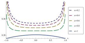
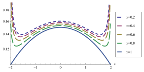
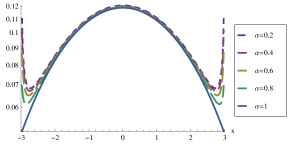
Figure 1. Plot of the absolutely continuous component of the distribution (4.19) for different values of $\alpha$, with $(c,\lambda)=(1,1)$ and $t=1$ (top left), $t=2$ (top right) $t=3$ (bottom). The figures are in logarithmic scale.

Remark 4.2.

Our approach consists in finding solutions of fractional Klein-Gordon equations and by means of them construct the probability distributions of fractional versions of finite-velocity random motions. We can see afterwards that the found solutions $p^{\alpha}(x,t)$ satisfy the same initial conditions as the classical telegraph process, i.e.

$$\begin{cases}p^{\alpha}(x,0)=\delta(x),\\ \frac{\partial p^{\alpha}}{\partial t}(x,t)\bigg{|}_{t=0}=0.\end{cases}$$

Remark 4.3.

For $\alpha=1$, the distribution (4.19) reduces to the sum of (4.4) (absolutely continuous component) and (4.5) (singular component).

Remark 4.4.

For all $k\geq 1$, there exists an order of fractionality $0<\alpha<1$ for which the conditional distributions are uniform in $[-ct,+ct]$. In particular, for all fixed values of $k\geq 0$, the distribution (4.18) is uniform for

$$\alpha=\frac{1}{2k+1},$$

while for values of $k\geq 1$, the distribution (4.16) is uniform for

$$\alpha=\frac{1}{k}.$$

The densities (4.18) for

$$0\leq k<\bigg{\lfloor}\frac{1-\alpha}{2\alpha}\bigg{\rfloor},$$

and the densities (4.16) for

$$1\leq k<\bigg{\lfloor}\frac{1}{\alpha}\bigg{\rfloor},$$

display an arcsine behaviour, that is, the densities approach to $+\infty$ for $x\rightarrow\pm ct$. In the opposite case, they have a bell-shaped form as happens with (4.2) and (4.3) for the classical telegraph process (see Fig. 1). This is an important feature of the fractional telegraph process.

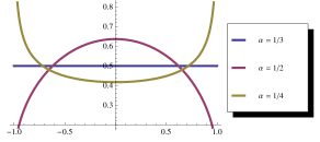
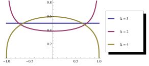
Figure 2. Plot of the conditional density (4.12) for $c=1$, $t=1$; Left side: $k=3$, $\alpha=(1/3,1/2,1/4)$, Right side: $\alpha=1/3$, $k=(3,2,4)$.

Lemma 4.5.

The function

(4.21) $$H(x,t) =E_{\alpha,1}(\lambda t^{\alpha})\sum_{k=0}^{\infty}P\{\mathcal{T}^{\alpha}\in dx|\mathcal{N}^{\alpha}(t)=2k+1\}P\{\mathcal{N}^{\alpha}(t)=2k+1\}$$

$$=\sum_{k=0}^{\infty}\left(\frac{\lambda}{2^{\alpha}c^{\alpha}}\right)^{2k+1}\frac{(c^{2}t^{2}-x^{2})^{\alpha k+\frac{\alpha-1}{2}}}{[\Gamma(\alpha k+\frac{1+\alpha}{2})]^{2}},$$

is a solution to the non-homogeneous fractional Klein–Gordon equation

(4.22) $$\left(\frac{\partial^{2}}{\partial t^{2}}-c^{2}\frac{\partial^{2}}{\partial x^{2}}\right)^{\alpha}u_{\alpha}(x,t)=\lambda^{2}u_{\alpha}(x,t)+\lambda 2^{\alpha}c^{\alpha}\frac{(\sqrt{c^{2}t^{2}-x^{2}})^{-\alpha-1}}{[\Gamma(\frac{1-\alpha}{2})]^{2}}.$$

Proof.

We start by writing the function $H$ in terms of the variable $w=\sqrt{c^{2}t^{2}-x^{2}}$.

$$H(w)=\sum_{k=0}^{\infty}\left(\frac{\lambda}{2^{\alpha}c^{\alpha}}\right)^{2k+1}\frac{w^{2\alpha k+\alpha-1}}{[\Gamma(\alpha k+\frac{1+\alpha}{2})]^{2}}.$$

By following some steps similar to those of Theorem 3.2 we have that

$$(L_{B})^{\alpha}H(w)=\frac{\lambda^{2}}{c^{2\alpha}}H(w)+\frac{\lambda 2^{\alpha}}{c^{\alpha}}\frac{w^{-\alpha-1}}{[\Gamma(\frac{1-\alpha}{2})]^{2}}.$$

Returning now to the original variables we obtain the claimed result. ∎

We can finally conclude with the following

Theorem 4.6.

The function

(4.23) $$f(x,t) =E_{\alpha,1}(\lambda t^{\alpha})\frac{P\{\mathcal{T}^{\alpha}(t)\in dx\}}{dx},\qquad x\in(-ct,+ct),$$

$$=\bigg{[}ct\sum_{k=1}^{\infty}\left(\frac{\lambda}{2^{\alpha}c^{\alpha}}\right)^{2k}\frac{(c^{2}t^{2}-x^{2})^{\alpha k-1}}{\Gamma(\alpha k)\Gamma(\alpha k+1)}+\sum_{k=0}^{\infty}\left(\frac{\lambda}{2^{\alpha}c^{\alpha}}\right)^{2k+1}\frac{(c^{2}t^{2}-x^{2})^{\alpha k+\frac{\alpha-1}{2}}}{[\Gamma(\alpha k+\frac{1+\alpha}{2})]^{2}}\bigg{]},$$

where $P\{\mathcal{T}^{\alpha}(t)\in dx\}/dx$ represents the absolutely continuous component of the distribution of the fractional telegraph process $\mathcal{T}^{\alpha}(t)$, $t\geq 0$, is a solution to the non-homogeneous fractional Klein–Gordon equation (4.22).

Proof.

The proof is a direct consequence of Theorem 3.7 and Lemma 4.5. ∎

5. Fractional planar random motion at finite velocity

A planar random motion at finite velocity with uniformly distributed orientation of displacements has been studied by several researchers over the years (see for example Stadje, 1987; Kolesnik and Orsingher, 2005). The motion is described by a particle taking directions $\theta_{j}$, $j=1,2,\dots$, (uniformly distributed in $(0,2\pi]$) at Poisson paced times. The orientations $\theta_{j}$ and the governing Poisson process $\mathcal{N}(t)$, $t\geq 0$, are assumed to be independent. The conditional distributions of the current position $(X(t),Y(t))$, $t\geq 0$, are given by (see formula (11) of Kolesnik and Orsingher (2005))

(5.1) $$P\{X(t)\in dx,Y(t)\in dy|\mathcal{N}(t)=n\}=\frac{n\left(c^{2}t^{2}-x^{2}-y^{2}\right)^{\frac{n}{2}-1}}{2\pi(ct)^{n}}dx\,dy,$$

for $x^{2}+y^{2}<c^{2}t^{2}$, $n\geq 1$, and possesses characteristic function

(5.2) $$\mathbb{E}\{e^{i\alpha X(t)+i\beta Y(t)}|\mathcal{N}(t)=n\}=\frac{2^{n/2}\Gamma(\frac{n}{2}+1)}{\left(ct\sqrt{\alpha^{2}+\beta^{2}}\right)^{n/2}}J_{\frac{n}{2}}\left(ct\sqrt{\alpha^{2}+\beta^{2}}\right),\qquad n\geq 1,\>(\alpha,\beta)\in\mathbb{R}^{2}.$$

The unconditional distribution of $(X(t),Y(t))$ reads

(5.3) $$P\{X(t)\in dx,Y(t)\in dy\}=\frac{\lambda}{2\pi c}\frac{e^{-\lambda t+\frac{\lambda}{c}\sqrt{c^{2}t^{2}-x^{2}-y^{2}}}}{\sqrt{c^{2}t^{2}-x^{2}-y^{2}}}dx\,dy,$$

for $x^{2}+y^{2}<c^{2}t^{2}$. The singular component of $(X(t),Y(t))$ is uniformly distributed on the circumference of radius $ct$ and has weight $e^{-\lambda t}$. It has been proven that the density in (5.3) is a solution to the planar telegraph equation (also equation of damped waves)

(5.4) $$\frac{\partial^{2}u}{\partial t^{2}}+2\lambda\frac{\partial u}{\partial t}=c^{2}\left\{\frac{\partial^{2}}{\partial x^{2}}+\frac{\partial^{2}}{\partial y^{2}}\right\}u.$$

In this section we construct a fractional planar random motion at finite velocity whose space-dependent component of the distribution solves the two-dimensional fractional Klein–Gordon equation

(5.5) $$\left(\frac{\partial^{2}}{\partial t^{2}}-c^{2}\left\{\frac{\partial^{2}}{\partial x^{2}}+\frac{\partial^{2}}{\partial y^{2}})\right\}\right)^{\alpha}u_{\alpha}(x,y,t)=\lambda^{2}u_{\alpha}(x,y,t),\quad\alpha\in(0,1].$$

By using the transformation

$$w=\sqrt{c^{2}t^{2}-x^{2}-y^{2}},$$

we convert (5.5) into the Bessel-type fractional equation

(5.6) $$\left(\frac{d^{2}}{dw^{2}}+\frac{2}{w}\frac{d}{dw}\right)^{\alpha}u_{\alpha}(w)=\frac{\lambda^{2}}{c^{2\alpha}}u_{\alpha}(w).$$

Since

(5.7) $$\left(\frac{d^{2}}{dw^{2}}+\frac{2}{w}\frac{d}{dw}\right)^{\alpha}=\left(\frac{1}{w^{2}}\frac{d}{dw}w^{2}\frac{d}{dw}\right)^{\alpha},$$

this operator coincides with (2.1) for $n=2$, $a_{1}=-2$, $a_{2}=2$, $a_{3}=0$. Therefore, in view of (2.4), $a=0$, $m=2$, $b_{1}=1/2$ and $b_{2}=0$, and, in view of (2.8), we can write

(5.8) $$\left(\frac{d^{2}}{dw^{2}}+\frac{2}{w}\frac{d}{dw}\right)^{\alpha}u_{\alpha}(w)=4^{\alpha}w^{-2\alpha}I_{2}^{0,-\alpha}I_{2}^{\frac{1}{2},-\alpha}u_{\alpha}(w).$$

We are now ready to state the following

Theorem 5.1.

A solution to (5.6) is given by

(5.9) $$u_{\alpha}(w) =\sum_{k=0}^{\infty}\left(\frac{\lambda}{c^{\alpha}}\right)^{2k+2}\frac{w^{2\alpha k+2\alpha-2}}{\Gamma(2\alpha k+2\alpha)}=\left(\frac{\lambda}{c^{\alpha}}\right)^{2}w^{2\alpha-2}E_{2\alpha,2\alpha}\left(\left(\frac{\lambda w^{\alpha}}{c^{\alpha}}\right)^{2}\right),\qquad w\in\mathbb{R},\>\alpha\in(0,1].$$

Proof.

We first observe that

(5.10) $$\left(\frac{d^{2}}{dw^{2}}+\frac{2}{w}\frac{d}{dw}\right)^{\alpha}w^{\beta} =4^{\alpha}w^{-2\alpha}I_{2}^{0,-\alpha}I_{2}^{\frac{1}{2},-\alpha}w^{\beta}=4^{\alpha}w^{-2\alpha}I_{2}^{0,-\alpha}\left(\frac{3}{2}-\alpha+\frac{\beta}{2}\right)\frac{\Gamma(\frac{1}{2}+1+\frac{\beta}{2})}{\Gamma(1-\alpha+\frac{1}{2}+\frac{\beta}{2}+1)}w^{\beta}$$

$$=4^{\alpha}w^{\beta-2\alpha}\left(\frac{3}{2}-\alpha+\frac{\beta}{2}\right)\left(1-\alpha+\frac{\beta}{2}\right)\frac{\Gamma(1+\frac{\beta}{2})\Gamma(\frac{1}{2}+1+\frac{\beta}{2})}{\Gamma(1-\alpha+\frac{1}{2}+\frac{\beta}{2}+1)\Gamma(1-\alpha+\frac{\beta}{2}+1)}$$

$$=4^{\alpha}w^{\beta-2\alpha}\frac{\Gamma(1+\frac{\beta}{2})\Gamma(\frac{1}{2}+1+\frac{\beta}{2})}{\Gamma(1-\alpha+\frac{1}{2}+\frac{\beta}{2})\Gamma(1-\alpha+\frac{\beta}{2})}=\frac{\Gamma(\beta+2)}{\Gamma(\beta+2-2\alpha)}w^{\beta-2\alpha},$$

where in view of (2.7) and in force of Lemma 3.1 we used the fact that

$$I^{\frac{1}{2},-\alpha}_{2}w^{\beta}=\left(\frac{3}{2}-\alpha+\frac{\beta}{2}\right)I_{2}^{\frac{1}{2},1-\alpha}w^{\beta}=\left(\frac{3}{2}-\alpha+\frac{\beta}{2}\right)\frac{\Gamma(\frac{1}{2}+\frac{\beta}{2}+1)}{\Gamma(1-\alpha+\frac{\beta}{2}+\frac{1}{2}+1)}w^{\beta}.$$

In the last step of (5.10) we repeatedly applied the duplication formula of the Gamma function. Hence we have that

$$\left(\frac{d^{2}}{dw^{2}}+\frac{2}{w}\frac{d}{dw}\right)^{\alpha}\sum_{k=0}^{\infty}\left(\frac{\lambda}{c^{\alpha}}\right)^{2k+2}\frac{w^{2\alpha k+2\alpha-2}}{\Gamma(2\alpha k+2\alpha)}$$

$$=\sum_{k=0}^{\infty}\left(\frac{\lambda}{c^{\alpha}}\right)^{2k+2}\frac{w^{2\alpha k-2}}{\Gamma(2\alpha k)}=\left(\frac{\lambda}{c^{\alpha}}\right)^{2}\sum_{k^{\prime}=0}^{\infty}\left(\frac{\lambda}{c^{\alpha}}\right)^{2k^{\prime}+2}\frac{w^{2\alpha k^{\prime}+2\alpha-2}}{\Gamma(2\alpha k^{\prime}+2\alpha)},$$

as claimed. ∎

Remark 5.2.

In light of Theorem 5.1 we can state that the two-dimensional fractional Klein–Gordon equation (5.5), admits the following solution:

(5.11) $$u_{\alpha}(x,y,t)=\left(\frac{\lambda}{c^{\alpha}}\right)^{2}\frac{E_{2\alpha,2\alpha}\left(\frac{\lambda^{2}}{c^{2\alpha}}(\sqrt{c^{2}t^{2}-x^{2}-y^{2}})^{2\alpha}\right)}{\left(\sqrt{c^{2}t^{2}-x^{2}-y^{2}}\right)^{2-2\alpha}},\qquad x^{2}+y^{2}<c^{2}t^{2}.$$

In the specific case $\alpha=1$, formula (5.11) takes the form

(5.12) $$u_{1}(x,y,t)=\sum_{k=0}^{\infty}\left(\frac{\lambda}{c}\right)^{2k+2}\frac{(\sqrt{c^{2}t^{2}-x^{2}-y^{2}})^{2k}}{(2k+1)!}.$$

The solution (5.11) of (5.5) can also be written as

$$u_{\alpha}(x,y,t)=\frac{2\pi c^{2\alpha}}{\lambda^{2}}E_{\alpha,1}(\lambda t^{\alpha})\sum_{k=0}^{\infty}P\{X^{\alpha}(t)\in dx,Y^{\alpha}(t)\in dy|\mathcal{N}^{\alpha}(t)=2k+2\}P\{\mathcal{N}^{\alpha}(t)=2k+2\},$$

where

$$P\{X^{\alpha}(t)\in dx,Y^{\alpha}\in dy|\mathcal{N}^{\alpha}(t)=2k+2\}=dx\,dy\frac{2k\alpha+2\alpha}{2\pi(ct)^{2k\alpha+2\alpha}}\left(\sqrt{c^{2}t^{2}-x^{2}-y^{2}}\right)^{2\alpha k+2\alpha-2},$$

for $k\geq 0,\,(x,y)\in C_{ct}$, and where

$$C_{ct}=\{(x,y)\in\mathbb{R}^{2}:x^{2}+y^{2}\leq c^{2}t^{2}\},$$

generalizes (5.1) for even values of $n$.

If $\mathcal{N}^{\alpha}(t)=2k+1$, we assume that

$$P\{X^{\alpha}(t)\in dx,Y^{\alpha}(t)\in dy|\mathcal{N}^{\alpha}(t)=2k+1\}$$

$$=dy\,dx\,(2k\alpha+\alpha)\left(\sqrt{c^{2}t^{2}-(x^{2}+y^{2})}\right)^{2\alpha k+\alpha-2}\Big{/}\left(2\pi(ct)^{2k\alpha+\alpha}\right),\qquad k\geq 0,\,(x,y)\in C_{ct}.$$

With all these preliminaries we arrive at the following theorem:

Theorem 5.3.

The vector process $(X^{\alpha}(t),Y^{\alpha}(t))$, $t\geq 0$, $0<\alpha\leq 1$, possesses the following probability distribution inside $C_{ct}$

(5.13) $$P\{X^{\alpha}(t)\in dx,Y^{\alpha}(t)\in dy\} =\frac{1}{2\pi E_{\alpha,1}(\lambda t^{\alpha})}\sum_{k=1}^{\infty}\left(\frac{\lambda}{c^{\alpha}}\right)^{k}\frac{(c^{2}t^{2}-x^{2}-y^{2})^{\alpha\frac{k}{2}-1}}{\Gamma(\alpha k)}$$

$$=\frac{\lambda}{2\pi c^{\alpha}E_{\alpha,1}(\lambda t^{\alpha})}\frac{E_{\alpha,\alpha}\left(\frac{\lambda}{c^{\alpha}}\left(\sqrt{c^{2}t^{2}-x^{2}-y^{2}}\right)^{\alpha}\right)}{\left(\sqrt{c^{2}t^{2}-x^{2}-y^{2}}\right)^{2-\alpha}}.$$

Proof.

From the previous calculations, we see that

(5.14) $$P\{X^{\alpha}(t)\in dx,Y^{\alpha}(t)\in dy|\mathcal{N}^{\alpha}(t)=n\}=\frac{\alpha n}{2\pi(ct)^{\alpha n}}\left(c^{2}t^{2}-x^{2}-y^{2}\right)^{\frac{n\alpha}{2}-1},\quad(x,y)\in C_{ct},$$

and thus we easily arrive at (5.13).

∎

Note that (5.13) coincides with (5.3) for $\alpha=1$.

Remark 5.4.

We observe that

$$\iint_{C_{ct}}P\{X^{\alpha}(t)\in dx,Y^{\alpha}(t)\in dy\}=\frac{1}{2\pi E_{\alpha,1}(\lambda t^{\alpha})}\sum_{k=1}^{\infty}\left(\frac{\lambda}{c^{\alpha}}\right)^{k}\int_{0}^{2\pi}\int_{0}^{ct}\frac{(c^{2}t^{2}-\rho^{2})^{\frac{\alpha k}{2}-1}\rho\,d\rho\,d\theta}{\Gamma(\alpha k)}$$

$$=\frac{1}{E_{\alpha,1}(\lambda t^{\alpha})}\sum_{k=1}^{\infty}\left(\frac{\lambda}{c^{\alpha}}\right)^{k}\frac{(ct)^{\alpha k}}{2}\int_{0}^{1}\frac{(1-y)^{\frac{\alpha k}{2}-1}dy}{\Gamma(\alpha k)}=\frac{1}{E_{\alpha,1}(\lambda t^{\alpha})}\sum_{k=1}^{\infty}\lambda^{k}t^{\alpha k}\frac{\bigg{[}(1-y)^{\frac{\alpha k}{2}}\bigg{]}^{0}_{1}}{\alpha k\Gamma(\alpha k)}$$

$$=1-\frac{1}{E_{\alpha,1}(\lambda t^{\alpha})}=1-P\{\mathcal{N}^{\alpha}(t)=0\},$$

This can be interpreted by observing that, if no Poisson event occurs, the particle performing the fractional planar motion arrives at $\partial C_{ct}$ with probability

$$P\{\mathcal{N}^{\alpha}(t)=0\}=1/E_{\alpha,1}(\lambda t^{\alpha}),$$

uniformly distributed on the circumference $\partial C_{ct}$ because of the initial uniformly distributed orientations of motion.

Remark 5.5.

A generalization of the planar random motion treated in Kolesnik and Orsingher (2005) and related to the fractional version treated above can be described as follows. A homogeneous Poisson process governs the changes of direction occurring at times $t_{j}$, with $0<t_{1}<\dots t_{j}<\dots<t_{n}<t$, of a particle moving with velocity $c$. At time $t_{j}$ the particle takes the orientation $\theta_{j}$ uniformly distributed in $[0,2\pi]$. The position $(\mathcal{X}(t),\mathcal{Y}(t))$ of the randomly moving particle, after $B(n,\alpha)$ changes of direction, reads

(5.15) $$\begin{cases}\mathcal{X}(t)=\displaystyle\sum\limits_{j=0}^{B(n,\alpha)}c\left(t_{j}-t_{j-1}\right)\cos\theta_{j},\\ \\ \mathcal{Y}(t)=\displaystyle\sum\limits_{j=0}^{B(n,\alpha)}c\left(t_{j}-t_{j-1}\right)\sin\theta_{j},\end{cases}$$

where $B(n,\alpha)$, $0<\alpha\leq 1$ is a binomial r.v. independent from $\theta_{j}$ and $t_{j}$, $0\leq j\leq B(n,\alpha)$. The conditional distribution of $(\mathcal{X}(t),\mathcal{Y}(t))$ reads

(5.16) $$P\{\mathcal{X}(t)\in dx,\mathcal{Y}(t)\in dy|\mathcal{N}(t)=B(n,\alpha)\}=\frac{B(n,\alpha)}{2\pi(ct)^{B(n,\alpha)}}\left(c^{2}t^{2}-x^{2}-y^{2}\right)^{\frac{B(n,\alpha)}{2}-1},$$

where $\mathcal{N}(t)$, $t\geq 0$ denotes the number of events in $[0,t]$ of a homogeneous Poisson process. This corresponds to randomize formula (11) of (Kolesnik and Orsingher, 2005) with $B(n,\alpha)$. In this case the parameter $\alpha$ is the order of the operator appearing in (5.5).
The mean value of (5.16) becomes

(5.17) $$\mathbb{E}P\{\mathcal{X}(t)\in dx,\mathcal{Y}(t)\in dy|\mathcal{N}(t)=B(n,\alpha)\} =\sum_{k=0}^{n}\frac{k\left(c^{2}t^{2}-x^{2}-y^{2}\right)^{\frac{k}{2}-1}}{2\pi(ct)^{k}}\binom{n}{k}\alpha^{k}(1-\alpha)^{n-k}$$

$$=\sum_{k=0}^{n}\frac{k\left[\sqrt{1-\frac{x^{2}+y^{2}}{c^{2}t^{2}}}\right]^{k}}{2\pi}\binom{n}{k}\frac{\alpha^{k}(1-\alpha)^{n-k}}{c^{2}t^{2}-x^{2}-y^{2}}$$

$$=\sum_{k=1}^{n}\frac{n!}{2\pi(n-k)!(k-1)!}\left(\alpha\sqrt{1-\frac{x^{2}+y^{2}}{c^{2}t^{2}}}\right)^{k}\frac{(1-\alpha)^{n-k}}{c^{2}t^{2}-x^{2}-y^{2}}$$

$$=\frac{n}{2\pi}\sum_{k=0}^{n-1}\binom{n-1}{k}\left(\alpha\sqrt{1-\frac{x^{2}+y^{2}}{c^{2}t^{2}}}\right)^{k+1}\frac{(1-\alpha)^{n-1-k}}{c^{2}t^{2}-x^{2}-y^{2}}$$

$$=\frac{n\alpha}{2\pi\sqrt{c^{2}t^{2}-x^{2}-y^{2}}}\frac{1}{(ct)^{n}}\left[ct+\alpha\left(\sqrt{c^{2}t^{2}-x^{2}-y^{2}}-ct\right)\right]^{n-1},$$

for $n\geq 1$. Note that, for $\alpha=1$ we retrieve distribution (5.1).

The unconditional distribution related to (5.17), obtained by randomizing $n$ with a fractional Poisson process $\mathcal{N}^{\alpha}(t)$, becomes

(5.18) $$P\{\mathcal{X}(t)\in dx,\mathcal{Y}(t)\in dy\} =\sum_{n=0}^{\infty}\mathbb{E}P\{\mathcal{X}(t)\in dx,\mathcal{Y}(t)\in dy|\mathcal{N}(t)=B(n,\alpha)\}P\{\mathcal{N}^{\alpha}(t)=n\}$$

$$=\frac{\lambda}{2\pi c}\frac{E_{\alpha,\alpha}\left(\frac{\lambda}{c}(ct+\alpha\{\sqrt{c^{2}t^{2}-x^{2}-y^{2}}-ct\})\right)}{\sqrt{c^{2}t^{2}-x^{2}-y^{2}}E_{\alpha,1}(\lambda t)}.$$

In the case where the process governing the number $n$ in the binomial r.v. of changes of direction is an homogeneous Poisson process, we have instead

(5.19) $$P\{X(t)\in dx,Y(t)\in dy\}=\frac{\lambda\alpha}{2\pi c}\frac{e^{-\frac{\lambda\alpha}{c}\left[ct-\sqrt{c^{2}t^{2}-x^{2}-y^{2}}\right]}}{\sqrt{c^{2}t^{2}-x^{2}-y^{2}}}.$$

Note that the following interesting inequality holds:

$$\mathbb{E}P\{\mathcal{X}(t)\in dx,\mathcal{Y}(t)\in dy|\mathcal{N}(t)=B(n,\alpha)\}\geq\alpha^{n}P\{X(t)\in dx,Y(t)\in dy|\mathcal{N}(t)=n\}.$$

We finally observe that the conditional distribution (5.14) of the fractional planar random motion

(5.20) $$P\{X^{\alpha}(t)\in dx,Y^{\alpha}(t)\in dy|\mathcal{N}^{\alpha}(t)=n\}=\frac{\alpha n}{2\pi(ct)^{\alpha n}}\left(c^{2}t^{2}-x^{2}-y^{2}\right)^{\frac{n\alpha}{2}-1},\quad(x,y)\in C_{ct},$$

can be obtained as

(5.21) $$P\{\mathcal{X}(t)\in dx,\mathcal{Y}(t)\in dy|\mathcal{N}(t)=\mathbb{E}(B(n,\alpha))=n\alpha\}.$$

Thus the fractionality implies that we take a fraction $\alpha$ of the number of changes of direction of the classical planar random motion.

Lemma 5.6.

The function

$$u_{\alpha}(w)=\sum_{k=0}^{\infty}\left(\frac{\lambda}{c^{\alpha}}\right)^{2k+1}\frac{w^{2k\alpha+\alpha-2}}{\Gamma(2k\alpha+\alpha)}=\frac{\lambda w^{\alpha-2}}{c^{\alpha}}E_{2\alpha,\alpha}\left(\frac{\lambda^{2}w^{2\alpha}}{c^{2\alpha}}\right),$$

is an analytic solution of the equation

(5.22) $$\left(\frac{d^{2}}{dw^{2}}+\frac{2}{w}\frac{d}{dw}\right)^{\alpha}u_{\alpha}(w)=\frac{\lambda^{2}}{c^{2\alpha}}u_{\alpha}(w)+\frac{\lambda}{c^{\alpha}}\frac{w^{-2-\alpha}}{\Gamma(-\alpha)}.$$

Proof.

In view of (5.10), we have that

$$\left(\frac{d^{2}}{dw^{2}}+\frac{2}{w}\frac{d}{dw}\right)^{\alpha}w^{2k\alpha+\alpha-2}=\frac{\Gamma(2k\alpha+\alpha)}{\Gamma(2k\alpha-\alpha)}w^{2k\alpha-\alpha-2}.$$

Hence

$$\left(\frac{d^{2}}{dw^{2}}+\frac{2}{w}\frac{d}{dw}\right)^{\alpha}u_{\alpha}(w) =\sum_{k=0}^{\infty}\left(\frac{\lambda}{c^{\alpha}}\right)^{2k+1}\frac{w^{2k\alpha-\alpha-2}}{\Gamma(2k\alpha-\alpha)}$$

$$=\left(\frac{\lambda}{c^{\alpha}}\right)^{2}\sum_{k^{\prime}=0}^{\infty}\left(\frac{\lambda}{c^{\alpha}}\right)^{2k^{\prime}+1}\frac{(w)^{2k^{\prime}\alpha+\alpha-2}}{\Gamma(2k^{\prime}\alpha+\alpha)}+\frac{\lambda}{c^{\alpha}}\frac{w^{-\alpha-2}}{\Gamma(-\alpha)}$$

$$=\left(\frac{\lambda}{c^{\alpha}}\right)^{2}u_{\alpha}(w)+\frac{\lambda}{c^{\alpha}}\frac{w^{-\alpha-2}}{\Gamma(-\alpha)},$$

as claimed. ∎

Corollary 5.7.

The function

(5.23) $$u_{\alpha}(x,y,t) =\frac{2\pi c^{\alpha}}{\lambda}E_{\alpha,1}(\lambda t^{\alpha})\sum_{k=0}^{\infty}P\{X^{\alpha}(t)\in dx,Y^{\alpha}(t)\in dy|\mathcal{N}^{\alpha}(t)=k\}P\{\mathcal{N}^{\alpha}(t)=k\}$$

$$=\sum_{k=0}^{\infty}\left(\frac{\lambda}{c^{\alpha}}\right)^{k}\frac{(\sqrt{c^{2}t^{2}-x^{2}-y^{2}})^{k\alpha-2}}{\Gamma(k\alpha)},$$

is an analytic solution to the non-homogeneous fractional Klein–Gordon equation

(5.24) $$\left(\frac{\partial^{2}}{\partial t^{2}}-c^{2}\left\{\frac{\partial^{2}}{\partial x^{2}}+\frac{\partial^{2}}{\partial y^{2}}\right\}\right)^{\alpha}u_{\alpha}(x,y,t)=\lambda^{2}u_{\alpha}(x,y,t)+\frac{\lambda c^{\alpha}\left(\sqrt{c^{2}t^{2}-x^{2}-y^{2}}\right)^{-\alpha-2}}{\Gamma(-\alpha)}.$$

Proof.

By splitting function (5.23) into even-order and odd-order terms and by considering Theorem 5.1 and Lemma 5.6, the result of corollary above immediately follows. ∎

We now study the distribution of the projection on the $x$-axis of the vector processes above, namely $X^{\alpha}_{p}(t)$, $t\geq 0$. We note that the distribution of $X^{\alpha}_{p}(t)$ possesses only the absolutely continuous component, unlike its two-dimensional counterpart. We first obtain

(5.25) $$\int_{-\sqrt{c^{2}t^{2}-x^{2}}}^{+\sqrt{c^{2}t^{2}-x^{2}}}\frac{k\alpha\left(\sqrt{c^{2}t^{2}-(x^{2}+y^{2})}\right)^{\alpha k-2}}{2\pi(ct)^{\alpha k}}dy =\frac{k\alpha\left(\sqrt{c^{2}t^{2}-x^{2}}\right)^{k\alpha-1}}{2\pi(ct)^{\alpha k}}\int_{0}^{1}\left(1-z\right)^{\frac{\alpha k}{2}-1}z^{-\frac{1}{2}}dz$$

$$=\frac{k\alpha\left(\sqrt{c^{2}t^{2}-x^{2}}\right)^{k\alpha-1}}{2\pi(ct)^{\alpha k}}\frac{\Gamma(\frac{k\alpha}{2})\Gamma(\frac{1}{2})}{\Gamma(\frac{k\alpha+1}{2})}$$

$$=\frac{\left(\sqrt{c^{2}t^{2}-x^{2}}\right)^{k\alpha-1}}{(2ct)^{\alpha k}}\frac{\Gamma(k\alpha+1)}{[\Gamma(\frac{k\alpha+1}{2})]^{2}},$$

where we used the fact that

$$\frac{k\alpha}{2}\Gamma\left(\frac{k\alpha}{2}\right)=\Gamma\left(\frac{k\alpha}{2}+\frac{1}{2}+\frac{1}{2}\right)=\frac{\Gamma(\frac{1}{2})2^{1-2(\frac{k\alpha+1}{2})}\Gamma(\alpha k+1)}{\Gamma(\frac{\alpha k+1}{2})}.$$

In view of (5.25) we extract the density

(5.26) $$p^{\alpha}(x,t) =\frac{1}{\pi\sqrt{c^{2}t^{2}-x^{2}}}\frac{1}{E_{\alpha,1}(\lambda t^{\alpha})}+\frac{1}{E_{\alpha,1}(\lambda t^{\alpha})}\frac{\lambda}{2^{\alpha}c^{\alpha}}\sum_{k=0}^{\infty}\left(\frac{\lambda}{2^{\alpha}c^{\alpha}}\right)^{k}\frac{\left(\sqrt{c^{2}t^{2}-x^{2}}\right)^{k\alpha+\alpha-1}}{[\Gamma(\frac{\alpha k+\alpha+1}{2})]^{2}}$$

$$=\frac{1}{E_{\alpha,1}(\lambda t^{\alpha})}\sum_{k=-1}^{\infty}\left(\frac{\lambda}{2^{\alpha}c^{\alpha}}\right)^{k+1}\frac{\left(\sqrt{c^{2}t^{2}-x^{2}}\right)^{k\alpha+\alpha-1}}{[\Gamma(\frac{\alpha k+\alpha+1}{2})]^{2}}$$

$$=\frac{1}{E_{\alpha,1}(\lambda t^{\alpha})}\sum_{k^{\prime}=0}^{\infty}\left(\frac{\lambda}{2^{\alpha}c^{\alpha}}\right)^{k^{\prime}}\frac{\left(\sqrt{c^{2}t^{2}-x^{2}}\right)^{k^{\prime}\alpha-1}}{[\Gamma(\frac{\alpha k^{\prime}+1}{2})]^{2}}$$

$$=\frac{1}{\sqrt{c^{2}t^{2}-x^{2}}}\frac{E_{2;\frac{\alpha}{2},\frac{1}{2}}\left(\frac{\lambda}{2^{\alpha}c^{\alpha}}(\sqrt{c^{2}t^{2}-x^{2}})^{\alpha}\right)}{E_{\alpha,1}(\lambda t^{\alpha})}.$$

We observe that the components of the planar fractional telegraph-type process have distributions without singular part because the singular part is projected on the $x$-axis. Moreover we notice that we recover for $\alpha=1$, the known case discussed, for example, by Orsingher and De Gregorio (2007).

Let us consider the function

(5.27) $$u_{\alpha}(x,t)=E_{\alpha,1}(\lambda t^{\alpha})p^{\alpha}(x,t)=\sum_{k=0}^{\infty}\left(\frac{\lambda}{2^{\alpha}c^{\alpha}}\right)^{k}\frac{(\sqrt{c^{2}t^{2}-x^{2}})^{k\alpha-1}}{[\Gamma(\frac{\alpha k+1}{2})]^{2}}.$$

For $u_{\alpha}(x,t)$, expressed in terms of $w=\sqrt{c^{2}t^{2}-x^{2}}$, we have the following theorem.

Theorem 5.8.

The function (5.27) is an analytic solution of the equation

(5.28) $$\left(\frac{d^{2}}{dw^{2}}+\frac{1}{w}\frac{d}{dw}\right)^{\alpha}u_{\alpha}(w)=\left(\frac{\lambda}{c^{\alpha}}\right)^{2}u_{\alpha}(w)+\frac{w^{-1-2\alpha}}{[\Gamma(\frac{1-2\alpha}{2})]^{2}}+\frac{\lambda}{c^{\alpha}}\frac{w^{-1-\alpha}}{[\Gamma(\frac{1-\alpha}{2})]^{2}}.$$

Proof.

By exploiting the relationship (3.8) for $\beta=\alpha k-1$, we arrive at (5.27). ∎

Remark 5.9.

We observe that in the case $\alpha=1$, the function

$$u_{1}(w)=\sum_{k=0}^{\infty}\left(\frac{\lambda}{2c}\right)^{k}\frac{w^{k-1}}{[\Gamma(\frac{k+1}{2})]^{2}},$$

is an analytic solution of the inhomogeneous Bessel-type equation

(5.29) $$\left(\frac{d^{2}}{dw^{2}}+\frac{1}{w}\frac{d}{dw}\right)u_{1}(w)=\frac{\lambda^{2}}{c^{2}}u_{1}(w)+\frac{1}{w^{3}[\Gamma(-\frac{1}{2})]^{2}}.$$

On the other hand, for $\alpha=1/2$, the first non-homogeneous term in (5.28) vanishes and we have that the function

(5.30) $$u_{1/2}(w)=\sum_{k=0}^{\infty}\left(\frac{\lambda}{2c}\right)^{k}\frac{w^{\frac{k}{2}-1}}{[\Gamma(\frac{k}{4}+\frac{1}{2})]^{2}}$$

is an analytic solution of the inhomogeneous Bessel-type equation

(5.31) $$\left(\frac{d^{2}}{dw^{2}}+\frac{1}{w}\frac{d}{dw}\right)^{1/2}u_{1/2}(w)=\frac{\lambda^{2}}{c}u_{1/2}(w)+\frac{\lambda}{\sqrt{c}}\frac{1}{\sqrt{w^{3}}[\Gamma(\frac{1}{4})]^{2}}.$$

6. $N$-Dimensional fractional random flights

We now treat the general $N$-dimensional fractional Klein–Gordon equation, i.e.

(6.1) $$\left(\frac{\partial^{2}}{\partial t^{2}}-c^{2}\Delta\right)^{\alpha}u_{\alpha}(\mathbf{x},t)=\lambda^{2}u_{\alpha}(\mathbf{x},t),\qquad\alpha\in(0,1],\>\mathbf{x}\in\mathbb{R}^{N}.$$

By means of the transformation

$$w=\left(c^{2}t^{2}-\sum_{k=1}^{N}x_{k}^{2}\right)^{1/2},$$

where $x_{k}$ is the $k$-th coordinate of the $N$-dimensional vector $\mathbf{x}$, we transform (6.1) in

(6.2) $$\left(\frac{d^{2}}{dw^{2}}+\frac{N}{w}\frac{d}{dw}\right)^{\alpha}u_{\alpha}(w)=\frac{\lambda^{2}}{c^{2\alpha}}u_{\alpha}(w).$$

The operator appearing in (6.2) can be considered again as a specific case of the operator (2.1) with $a_{1}=-N$, $a_{2}=N$, $a_{3}=0$, $a=0$, $n=m=2$, $b_{1}=\frac{N-1}{2}$ and $b_{2}=0$. Hence, from (2.8) we have that

(6.3) $$\left(\frac{d^{2}}{dw^{2}}+\frac{N}{w}\frac{d}{dw}\right)^{\alpha}u_{\alpha}(w)=4^{\alpha}w^{-2\alpha}I_{2}^{0,-\alpha}I_{2}^{\frac{N-1}{2},-\alpha}u_{\alpha}(w).$$

We are now ready to state the following

Theorem 6.1.

A solution to (6.2) is given by

(6.4) $$u_{\alpha}(w)=\sum_{k=0}^{\infty}\left(\frac{\lambda}{2^{\alpha}c^{\alpha}}\right)^{2k}\frac{w^{2\alpha k+2\alpha-2}}{\Gamma(\alpha k+\alpha+\frac{N-1}{2})\Gamma(\alpha k+\alpha)}.$$

Proof.

We first observe that

$$\left(\frac{d^{2}}{dw^{2}}+\frac{N}{w}\frac{d}{dw}\right)^{\alpha}w^{\beta}=4^{\alpha}w^{-2\alpha}I_{2}^{0,-\alpha}I_{2}^{\frac{N-1}{2},-\alpha}w^{\beta}$$

$$=4^{\alpha}w^{-2\alpha}I_{2}^{0,-\alpha}\left(\frac{N-1}{2}+1-\alpha+\frac{\beta}{2}\right)\frac{\Gamma(\frac{N-1}{2}+1+\frac{\beta}{2})}{\Gamma(1-\alpha+\frac{N-1}{2}+\frac{\beta}{2}+1)}w^{\beta}$$

$$=4^{\alpha}w^{-2\alpha}\left(1-\alpha+\frac{\beta}{2}\right)\left(\frac{N-1}{2}+1-\alpha+\frac{\beta}{2}\right)\frac{\Gamma(\frac{\beta}{2}+1)}{\Gamma(1-\alpha+\frac{\beta}{2}+1)}\frac{\Gamma(\frac{N-1}{2}+1+\frac{\beta}{2})}{\Gamma(1-\alpha+\frac{N-1}{2}+\frac{\beta}{2}+1)}w^{\beta}$$

$$=4^{\alpha}w^{\beta-2\alpha}\frac{\Gamma(\frac{\beta}{2}+1)}{\Gamma(1-\alpha+\frac{\beta}{2})}\frac{\Gamma(\frac{N-1}{2}+1+\frac{\beta}{2})}{\Gamma(1-\alpha+\frac{N-1}{2}+\frac{\beta}{2})}.$$

Hence we have that

$$\left(\frac{d^{2}}{dw^{2}}+\frac{N}{w}\frac{d}{dw}\right)^{\alpha}\sum_{k=0}^{\infty}\left(\frac{\lambda}{2^{\alpha}c^{\alpha}}\right)^{2k}\frac{w^{2\alpha k+2\alpha-2}}{\Gamma(\alpha k+\alpha+\frac{N-1}{2})\Gamma(\alpha k+\alpha)}$$

$$=4^{\alpha}\sum_{k=0}^{\infty}\left(\frac{\lambda}{2^{\alpha}c^{\alpha}}\right)^{2k}\frac{w^{2\alpha k-2}}{\Gamma(\alpha k+\frac{N-1}{2})\Gamma(\alpha k)}$$

$$=\left(\frac{\lambda}{c^{\alpha}}\right)^{2}\sum_{k^{\prime}=0}^{\infty}\left(\frac{\lambda}{2^{\alpha}c^{\alpha}}\right)^{2k^{\prime}}\frac{w^{2\alpha k^{\prime}+2\alpha-2}}{\Gamma(\alpha k^{\prime}+\alpha+\frac{N-1}{2})\Gamma(\alpha k^{\prime}+\alpha)},$$

as claimed. ∎

Remark 6.2.

From Theorem 6.1, writing the function (6.4) in terms of the variables $(\mathbf{x},t)$, we have that

(6.5) $$u_{\alpha}(\mathbf{x},t)=\sum_{k=0}^{\infty}\left(\frac{\lambda}{2^{\alpha}c^{\alpha}}\right)^{2k}\frac{\left(\sqrt{c^{2}t^{2}-\sum_{k=1}^{N}x_{k}^{2}}\right)^{2\alpha k+2\alpha-2}}{\Gamma(\alpha k+\alpha+\frac{N-1}{2})\Gamma(\alpha k+\alpha)}$$

solves the $N$-dimensional fractional Klein–Gordon equation

(6.6) $$\left(\frac{\partial^{2}}{\partial t^{2}}-c^{2}\Delta\right)^{\alpha}u_{\alpha}(\mathbf{x},t)=\lambda^{2}u_{\alpha}(\mathbf{x},t).$$

Moreover, for $N=1$ and $N=2$, we recover the results found above, up to a multiplicative term.

Remark 6.3.

Inspired by Theorem 6.1, we construct a fractional extension of the random flight in $\mathbb{R}^{4}$, previously studied in Orsingher and De Gregorio (2007). For the vector process $\mathbf{X}(t)=(X_{1}(t),X_{2}(t),X_{3}(t),X_{4}(t))$ we write

(6.7) $$P\Biggl{\{}\bigcap_{j=1}^{4}\{X_{j}(t)\in dx_{j}\}\Bigr{|}\mathcal{N}^{\alpha/2}(t)=k\Biggr{\}}=\frac{\left(\frac{k\alpha}{2}+1\right)\frac{k\alpha}{2}\left(\sqrt{c^{2}t^{2}-\|\mathbf{x}\|^{2}}\right)^{k\alpha-2}}{\pi^{2}(ct)^{k\alpha+2}}\prod_{j=1}^{4}dx_{j},$$

for $\alpha\in(1,2]$ and $\|\mathbf{x}\|^{2}\leq c^{2}t^{2}$. We note that, for $\alpha=2$, (6.7) coincides with formula (1.5) of Orsingher and De Gregorio (2007). The distribution of the fractional Poisson process $\mathcal{N}^{\alpha/2}(t)$, $t\geq 0$, reads

(6.8) $$P\{\mathcal{N}^{\alpha/2}(t)=k\}=\frac{\left(\lambda t^{\alpha/2}\right)^{k}}{\Gamma\left(\frac{k\alpha}{2}+1\right)}\frac{1}{E_{\alpha/2,1}(\lambda t^{\alpha/2})},\qquad k\geq 0,\>\alpha\in(1,2].$$

The absolutely continuous component of the distribution of $\mathbf{X}(t)$ is given by

(6.9) $$p^{\alpha}(\mathbf{x},t)=\sum_{k=0}^{\infty}\frac{\left(\frac{k\alpha}{2}+1\right)\frac{k\alpha}{2}\left(\sqrt{c^{2}t^{2}-\|\mathbf{x}\|^{2}}\right)^{k\alpha-2}}{\pi^{2}(ct)^{k\alpha+2}}\frac{\left(\lambda t^{\alpha/2}\right)^{k}}{\Gamma\left(\frac{k\alpha}{2}+1\right)}\frac{1}{E_{\alpha/2,1}(\lambda t^{\alpha/2})}$$

$$=\frac{1}{\pi^{2}E_{\alpha/2,1}(\lambda t^{\frac{\alpha}{2}})(ct)^{2}}\left[\sum_{k=0}^{\infty}\left(\frac{\lambda}{c^{\alpha}t^{\alpha/2}}\right)^{k}\frac{\left(\sqrt{c^{2}t^{2}-\|\mathbf{x}\|^{2}}\right)^{k\alpha-2}}{\Gamma\left(\frac{k\alpha}{2}-1\right)}+2\sum_{k=0}^{\infty}\left(\frac{\lambda}{c^{\alpha}t^{\alpha/2}}\right)^{k}\frac{\left(\sqrt{c^{2}t^{2}-\|\mathbf{x}\|^{2}}\right)^{k\alpha-2}}{\Gamma\left(\frac{k\alpha}{2}\right)}\right]$$

$$=\frac{\lambda}{\pi^{2}c^{2+\alpha}t^{2+\alpha/2}E_{\alpha/2,1}(\lambda t^{\alpha/2})\left(\sqrt{c^{2}t^{2}-\|\mathbf{x}\|^{2}}\right)^{2-\alpha}}\bigg{[}E_{\alpha/2,\alpha/2-1}\left(\frac{\lambda}{c^{\alpha}t^{\alpha/2}}\left(\sqrt{c^{2}t^{2}-\|\mathbf{x}\|^{2}}\right)^{\alpha}\right)$$

$$\quad+2E_{\alpha/2,\alpha/2}\left(\frac{\lambda}{c^{\alpha}t^{\alpha/2}}\left(\sqrt{c^{2}t^{2}-\|\mathbf{x}\|^{2}}\right)^{\alpha}\right)\bigg{]}.$$

For $\alpha=2$, formula (6.9) coincides with (3.7) of Orsingher and De Gregorio (2007), since

$$E_{1,0}(x)=xe^{x},\qquad E_{1,1}(x)=e^{x}.$$

The fractional random flight in $\mathbb{R}^{4}$ can be viewed as a motion with a binomial number $B(n,\frac{\alpha}{2})$ of changes of orientations (uniformly distributed on the hypersphere), where $n$ possesses fractional Poisson distribution given by (6.8). The conditional distribution (6.7) is thus written as (see Remark 5.5 for the planar case)

$$P\Biggl{\{}\bigcap_{j=1}^{4}\{X_{j}(t)\in dx_{j}\}\Bigr{|}\mathcal{N}(t)=\mathbb{E}B\left(n,\frac{\alpha}{2}\right)\Biggr{\}}.$$

7. Higher order cases

We devote this section to the fractional hyper-Bessel operators

(7.1) $$(L_{B_{n}})^{\alpha}=\Biggl{(}\frac{1}{w^{n}}\Biggl{(}\underbrace{w\frac{d}{dw}w\frac{d}{dw}\dots w\frac{d}{dw}}_{\text{$n$ times}}\Biggr{)}\Biggr{)}^{\alpha},\qquad\alpha\in(0,1].$$

We first treat in detail the fractional third-order Bessel equation:

(7.2) $$(L_{B_{3}})^{\alpha}f(w)=\left(\frac{1}{w^{2}}\frac{d}{dw}+\frac{3}{w}\frac{d^{2}}{dw^{2}}+\frac{d^{3}}{dw^{3}}\right)^{\alpha}f(w)=\left(\frac{\lambda}{c^{\alpha}}\right)^{3}f(w).\qquad\alpha\in(0,1].$$

The operator $L_{B_{3}}$ coincides with (2.1), for $n=3$, $a_{1}=-2$, $a_{2}=a_{3}=1$, $a_{4}=0$. Therefore, in view of Lemma 2.1, we obtain that $a=0$, $m=3$, $b_{1}=b_{2}=b_{3}=0$. Indeed

$$L_{B_{3}}=\frac{1}{w^{2}}\frac{d}{dw}\left(w\frac{d}{dw}\right)^{2}.$$

Therefore

(7.3) $$\left(\frac{1}{w^{2}}\frac{d}{dw}+\frac{3}{w}\frac{d^{2}}{dw^{2}}+\frac{d^{3}}{dw^{3}}\right)^{\alpha}f(w) =3^{3\alpha}w^{-3\alpha}\prod_{k=1}^{3}I_{3}^{b_{k},-\alpha}f(w)$$

$$=3^{3\alpha}w^{-3\alpha}I_{3}^{0,-\alpha}I_{3}^{0,-\alpha}I_{3}^{0,-\alpha}f(w).$$

Theorem 7.1.

Let $\alpha\in(0,1]$, then the equation

$$\left(\frac{1}{w^{2}}\frac{d}{dw}+\frac{3}{w}\frac{d^{2}}{dw^{2}}+\frac{d^{3}}{dw^{3}}\right)^{\alpha}f(w)=f(w),\quad w\in\mathbb{R},$$

is satisfied by

(7.4) $$f(w)=w^{3\alpha-3}\sum_{k=0}^{\infty}\left(\frac{w}{3}\right)^{3\alpha k}\frac{1}{[\Gamma(\alpha k+\alpha)]^{3}}.$$

Proof.

We first observe that for $\beta>0$

(7.5) $$(L_{B_{3}})^{\alpha}w^{\beta} =3^{3\alpha}w^{-3\alpha}I_{3}^{0,-\alpha}I_{3}^{0,-\alpha}I_{3}^{0,-\alpha}w^{\beta}$$

$$=3^{3\alpha}w^{-3\alpha}\left[(1-\alpha)I_{3}^{0,1-\alpha}+\frac{1}{3}I_{3}^{0,1-\alpha}\left(w\frac{d}{dx}\right)\right]^{3}w^{\beta}$$

$$=3^{3\alpha}w^{-3\alpha}(1-\alpha+\frac{1}{3}\beta)^{3}I_{3}^{0,1-\alpha}I_{3}^{0,1-\alpha}I_{3}^{0,1-\alpha}w^{\beta}$$

$$=3^{3\alpha}w^{-3\alpha}(1-\alpha+\frac{1}{3}\beta)^{3}\left[\frac{\Gamma\left(\frac{\beta}{3}+1\right)}{\Gamma\left(1-\alpha+1+\frac{\beta}{3}\right)}\right]^{3}w^{\beta}$$

$$=3^{3\alpha}\left[\frac{\Gamma\left(\frac{\beta}{3}+1\right)}{\Gamma\left(1-\alpha+\frac{\beta}{3}\right)}\right]^{3}w^{\beta-3\alpha}.$$

Then we immediately have

$$(L_{B_{3}})^{\alpha}\left(w^{3\alpha-3}\sum_{k=0}^{\infty}\frac{1}{3^{3\alpha k}}\frac{w^{3\alpha k}}{[\Gamma(\alpha k+\alpha)]^{3}}\right)=3^{3\alpha}\sum_{k=0}^{\infty}\frac{1}{3^{3\alpha k}}\frac{w^{3\alpha k-3}}{[\Gamma(\alpha k)]^{3}}=\sum_{k^{\prime}=0}^{\infty}\frac{1}{3^{3\alpha k}}\frac{w^{3\alpha k^{\prime}+3\alpha-3}}{[\Gamma(\alpha k^{\prime}+\alpha)]^{3}}.$$

∎

We finally arrive at the general theorem that can be easily proved as the preceding one.

Theorem 7.2.

Let be $\alpha\in(0,1]$, $n\in\mathbb{N}$. The equation

(7.6) $$\left(\frac{1}{w^{n}}\left(w\frac{d}{dw}\right)^{n}\right)^{\alpha}f(w)=f(w),$$

is satisfied by

(7.7) $$f(w)=w^{n\alpha-n}\sum_{k=0}^{\infty}\left(\frac{w}{n}\right)^{n\alpha k}\frac{1}{[\Gamma(\alpha k+\alpha)]^{n}}.$$

Remark 7.3.

We observe that the fractional higher order equation

(7.8) $$\left(\frac{1}{w^{2}}\frac{d}{dw}+\frac{3}{w}\frac{d^{2}}{dw^{2}}+\frac{d^{3}}{dw^{3}}\right)^{\alpha}f(w)=\left(\frac{\sqrt[3]{6}\lambda}{c}\right)^{3\alpha}f(w)$$

is directly related to the fractional partial differential equation in $2+1$ variables

(7.9) $$\left(\frac{\partial}{\partial t}+c\frac{\partial^{\alpha}}{\partial x}\right)^{\alpha}\left(\frac{\partial}{\partial t}-\frac{c}{2}\frac{\partial}{\partial x}+\frac{c\sqrt{3}}{2}\frac{\partial}{\partial y}\right)^{\alpha}\left(\frac{\partial}{\partial t}-\frac{c}{2}\frac{\partial}{\partial x}-\frac{c\sqrt{3}}{2}\frac{\partial}{\partial y}\right)^{\alpha}u_{\alpha}(x,y,t)=\lambda^{3}u_{\alpha}(x,y,t).$$

Indeed it can be obtained from (7.9) by a sequence of two transformations (see Orsingher (2002)). The first one is

$$\begin{cases}z_{1}=\frac{ct}{2}+x,\\ z_{2}=\frac{ct-x}{\sqrt{3}}+y,\\ z_{3}=\frac{ct-x}{\sqrt{3}}-y,\end{cases}$$

that reduces (7.9) to

(7.10) $$\left(\frac{9c^{3}}{2}\frac{\partial}{\partial z_{1}}\frac{\partial}{\partial z_{2}}\frac{\partial}{\partial z_{3}}\right)^{\alpha}u_{\alpha}(z_{1},z_{2},z_{3})=\lambda^{3}u_{\alpha}(z_{1},z_{2},z_{3}).$$

Then, by means of a second transformation $w=\sqrt[3]{z_{1}z_{2}z_{3}}$, we obtain (7.8). In turn, by considering

$$w^{\prime}=\frac{\sqrt[3]{6}\lambda w}{c},$$

the equation (7.8) can be converted in (7.6). Therefore the solution of (7.9) can be written as

(7.11) $$u_{\alpha}(x,y,t)=\sum_{k=0}^{\infty}\left(\frac{\lambda}{3c}\sqrt[3]{(ct+3x)[(ct-x)^{2}-3y^{2}]}\right)^{3\alpha k+3\alpha-3}\frac{1}{[\Gamma(\alpha k+\alpha]^{3}}.$$

A specific case of (7.11) for $\alpha=1$ reads

(7.12) $$I_{0,3}\left(\frac{\lambda}{c}\sqrt[3]{(ct+3x)[(ct-x)^{2}-3y^{2}]}\right),$$

where

$$I_{0,3}(x)=\sum_{k=0}^{\infty}\left(\frac{x}{3}\right)^{3k}\frac{1}{(k!)^{3}},$$

is the third-order Bessel function.

Equation (7.9) emerges in the study of a planar cyclic random motion with three directions (Orsingher, 2002). The fractional version of this random motion can be obtained from its integer counterpart by introducing a randomization of the number of changes of direction as done in the previously analyzed cases.

8. An application to the fractional Euler–Poisson–Darboux equation

We now introduce the following fractional formulation of the classical Euler–Poisson–Darboux equation (see for example Samko et al., 1993)

(8.1) $$\left(\frac{1}{t^{\chi}}\frac{\partial}{\partial t}t^{\chi}\frac{\partial}{\partial t}\right)^{\alpha}f(\mathbf{x},t)=\left(\frac{\partial^{2}}{\partial t^{2}}+\frac{\chi}{t}\frac{\partial}{\partial t}\right)^{\alpha}f(\mathbf{x},t)=\Delta f(\mathbf{x},t),$$

where $\alpha\in(0,1]$, $t\geq 0$, $\mathbf{x}\in\mathbb{R}^{N}$ and $\chi\in\mathbb{R}$. Clearly the operator appearing in (8.1) is a special case of (2.1), with $n=2$, $a_{1}=-\chi$, $a_{2}=\chi$ and $a_{3}=0$. In the following we take for simplicity $\chi=1$. This is a fractional generalization of the classical equation that is recovered for $\alpha=1$. Using the formalism used in the previous section, we can write (8.1) in a compact way as

(8.2) $$(L_{B})_{t}^{\alpha}f(\mathbf{x},t)=\Delta f(\mathbf{x},t).$$

Applying the Fourier transform we have

(8.3) $$(L_{B})_{t}^{\alpha}f(\mathbf{k},t)=|\mathbf{k}|^{2}f(\mathbf{k},t),$$

whose solution is given by

(8.4) $$f(\mathbf{k},t)=t^{2\alpha-2}\sum_{j=0}^{\infty}\left[\left(\frac{t}{2}\right)^{\alpha}|\mathbf{k}|\right]^{2j}\frac{1}{[\Gamma(\alpha j+\alpha)]^{2}}.$$

In more general, but rather formal way, we have the following

Theorem 8.1.

Consider the initial value problem (IVP)

(8.5) $$\begin{cases}\left(\frac{\partial^{2}}{\partial t^{2}}+\frac{1}{t}\frac{\partial}{\partial t}\right)^{\alpha}f(x,t)=\widehat{O}_{x}f(x,t),&t>0,\\ f(x,0)=g(x),\end{cases}$$

where $\widehat{O}_{x}$ is an integro-differential operator acting on the space variable that satisfies the semigroup property and $g(x)$ is an analytic function. Then the operational solution of equation (8.5) is given by:

(8.6) $$f(x,t)=t^{2\alpha-2}\sum_{j=0}^{\infty}\left(\frac{t}{2}\right)^{2\alpha j}\frac{\widehat{O}_{x}^{j}\,g(x)}{[\Gamma(\alpha j+\alpha)]^{2}}$$

The operational solution (8.6) becomes an effective solution when the series converges, and this depends upon the actual form of the initial condition $g(x)$. Operational methods to solve Euler–Poisson–Darboux equations are applied in Olevskii (2004).

Acknowledgement. We are very greatful to both referees for their suggestions and, in particular, to reviewer $\sharp 1$ for insightful remarks and for checking many calculations.

References

Balakrishnan and Kozubowski (2008) N. Balakrishnan, T.J. Kozubowski.
A class of weighted Poisson processes, Statistics and Probability Letters, 78(15):2346–2352, (2008)
Beghin and Orsingher (2009) L. Beghin, E. Orsingher.
Fractional Poisson processes
and related planar random motions, Electronic Journal of Probability, 14(61):1790–1826, (2009)
Bollini and Giambiagi (1993) C.G. Bollini, J.J. Giambiagi.
Arbitrary powers of D’Alembertians and
the Huygens’ principle, Journal of Mathematical Physics, 34(2):610–621, (1993)
De Gregorio et al. (2005) A. De Gregorio, E. Orsingher, L. Sakhno.
Motions with finite velocity
analyzed with order statistics and differential equations,
Theory of Probability and Mathematical Statistics, 71:63–79, (2005)
Garra and Polito (2013) R. Garra, F. Polito. On some operators involving Hadamard derivatives,
Integral transform and special functions, 24(10): 773-782, (2013)
Kiryakova (2000) V. Kiryakova.
Multiple (multiindex) Mittag–Leffler functions
and relations to generalized fractional calculus,
Journal of Computational and Applied Mathematics, 118(1–2):241–259, (2000)
Kolesnik and Orsingher (2005) A.D. Kolesnik, E .Orsingher.
A planar random motion with an
infinite number of directions controlled by the damped
wave equation, Journal of Applied Probability,
42(4):1168–1182, (2005)
Lachal et al. (2006) A. Lachal, S. Leorato, E. Orsingher.
Minimal cyclic random motion in and hyper-Bessel functions,
Annales de l’Institut Henri Poincaré (B) Probability and Statistics, 42(6):753–772, (2006)
Lim and Muniandy (2004) S.C. Lim, S.V. Muniandy.
Stochastic quantization of nonlocal fields,
Physics Letters A, 324(5–6):396–405, (2004)
McBride (1982) A.C. McBride. Fractional Powers of a Class of Ordinary Differential Operators,
Proceedings of the London Mathematical Society, 3(45):519–546, (1982)
McBride (1975) A.C. McBride. A theory of fractional integration for generalized functions,
SIAM Journal on Mathematical Analysis, 6(3):583–599, (1975)
McBride (1979) A.C. McBride. Fractional calculus and integral transforms
of generalised functions, Pitman, London, (1979)
Olevskii (2004) M.N. Olevskii,
An Operator Approach to the Cauchy Problem for the Euler–Poisson–Darboux Equation
in Spaces of Constant Curvature, Integral Equations and Operator Theory, 49(1):77–109, (2004)
Orsingher (2002) E. Orsingher. Bessel functions of third
order and the distribution of cyclic planar motions
with three directions, Stochastics and Stochastics Reports, 74(3–4):617–631, (2002)
Orsingher and Beghin (2004) E. Orsingher, L. Beghin.
Time-fractional telegraph equations and telegraph processes with Brownian time,
Probability Theory and Related Fields, 128(1):141–160, (2004)
Orsingher and De Gregorio (2007) E. Orsingher, A. De Gregorio.
Random flights in higher spaces,
Journal of Theoretical Probability, 20(4):769–806, (2007)
Orsingher and Toaldo (2013) E. Orsingher, B.
Toaldo, Time-changed processes governed by space-time fractional telegraph equations
Preprint arXiv:1206.2511, (2013)
Podlubny (1999) I. Podlubny. Fractional Differential Equations,
Academic Press, New York, (1999)
Samko et al. (1993) S.G. Samko, A.A. Kilbas, O.I. Marichev.
Fractional integrals and derivatives, Gordon and Breach Science, Yverdon, Switzerland (1993)
Schiavone and Lamb (1990) S.E. Schiavone, W. Lamb.
A fractional power approach to fractional
calculus, Journal of Mathematical Analysis and
Applications, 149(2):377–401, (1990)
Stadje (1987) W. Stadje. The exact probability distribution of a two-dimensional random walk,
Journal of Statistical Physics, 46(1–2):207–216, (1987)
Yakubovich and Luchko (1994) S.B. Yakubovich and Y.F. Luchko.
The hypergeometric approach to integral transforms and convolutions,
Kluwer Academic Publishers, Dordrecht, (1994)