Two-loop QED corrections with closed fermion loops for the bound-electron $\bm{g}$ factor

Abstract

Two-loop QED corrections with closed fermion loops are calculated for the $1s$ bound-electron $g$ factor. Calculations are performed to all orders in the nuclear binding strength parameter $Z\alpha$ (where $Z$ is the nuclear charge and $\alpha$ is the fine structure constant) except for the closed fermion loop, which is treated within the free-loop (Uehling) approximation in some cases. Comparison with previous $Z\alpha$-expansion calculations is made and the higher-order remainder of order $\alpha^{2}(Z\alpha)^{5}$ and higher is separated out from the numerical results.

Highly charged ions are often considered to be an ideal testing ground for studying bound-state quantum electrodynamics (QED) effects, in particular, the effects that are non-perturbative in the binding nuclear strength parameter $Z\alpha$ (where $Z$ is the nuclear charge, $\alpha$ is the fine structure constant). For light atomic systems, the parameter $Z\alpha$ is small and the $Z\alpha$ expansion is widely used as a convenient basis for theoretical calculations. However, high accuracy achieved in modern experiments often demands calculations of QED corrections beyond the $Z\alpha$ expansion even for light atoms. For heavy highly charged ions, the $Z\alpha$ expansion is not applicable at all and calculations should be only carried out to all orders in $Z\alpha$.

One of the prominent examples of experiments in light atoms that require for their interpretation calculations of QED effects to all orders in $Z\alpha$ is the determination of the bound-electron $g$ factor in hydrogenlike ions. A series of spectacular measurements has been accomplished during the last two decades haeffner:00:prl ; verdu:04 ; sturm:11 ; sturm:13:Si ; wagner:13 , which brought the experimental accuracy on the level of few parts in $10^{-11}$. These measurements triggered a large number of calculations of various QED effects that were required for advancing theory to the level of experimental interest. In particular, all-order (in $Z\alpha$) calculations of the one-loop self-energy yerokhin:02:prl and nuclear recoil shabaev:02:recprl corrections were accomplished, as well as $Z\alpha$-expansion calculations of the two-loop QED effects pachucki:04:prl ; pachucki:05:gfact . The comparison between the experimental and the theoretical results not only constituted a highly sensitive test of bound-state QED theory but also led to an accurate determination of fundamental physical constants such as the electron mass beier:02:prl ; mohr:13:codata .

Despite all theoretical efforts, the present theory of the bound-electron $g$ factor is not able to match the experimental accuracy for the heaviest measured ion, Si¹³⁺ sturm:13:Si . The main reason for this are the two-loop QED effects, which are presently calculated within the $Z\alpha$ expansion up to order $\alpha^{2}(Z\alpha)^{4}$ only. The uncertainty due to unknown higher-order two-loop effects induces the dominant error in the theoretical prediction for ions with $Z>6$. For silicon with $Z=14$, this uncertainty is already by more than an order of magnitude larger than the experimental error sturm:13:Si . Scaling as $Z^{5}$, it is going to become even more crucial for comparison of theory with experiments on heavier-$Z$ ions, which should become feasible in the near future sturm:11:prl .

Calculation of the two-loop QED corrections to all orders in the nuclear binding strength parameter $Z\alpha$ is a very difficult task. Such calculation for the Lamb shift in hydrogenlike ions extended for over a decade (see Refs. yerokhin:08:twoloop ; yerokhin:09:sese ; yerokhin:10:sese for the present status). A similar calculation for the bound-electron $g$ factor should be feasible in principle but is going to be even more difficult than for the Lamb shift, for several reasons. First, Feynman diagrams for the $g$ factor contain an additional vertex representing the interaction with the external magnetic field as compared to the diagrams contributing to the Lamb shift. Second, the convergence of the partial-wave expansion (which is usually the limiting factor for the accuracy of calculations) is typically slower for the $g$ factor than for the Lamb shift. Third, the unknown higher-order remainder to the Lamb shift is suppressed by the factor of $(Z\alpha)^{2}$ with respect to the leading contribution, whereas for the $g$ factor the suppression factor is $(Z\alpha)^{5}$.

The two-loop QED effects can be separated into two large pieces, the two-loop self-energy correction and the two-loop corrections with closed fermion (vacuum-polarization) loops. In the present study, we consider the latter part, leaving the two-loop self-energy (being the most nontrivial part) for future investigations. Calculations of the two-loop corrections with vacuum-polarization loops are simplified by the fact that such loops can be treated within the free-loop (Uehling) approximation, which replaces the loop of the bound-electron propagators by the leading term of its expansion in the binding potential. In the one-loop case, such approximation leads to the well-known Uehling potential and induces the dominant part of the one-loop vacuum-polarization effect even for ions as heavy as uranium. In the present investigation, we employ the free-loop approximation for some corrections, namely the self-energy correction with the vacuum-polarization insertion into the photon line and the two-loop vacuum-polarization correction. In addition, there are several diagrams that vanish in the free-loop approximation, namely the diagrams with the interaction with the external magnetic field attached to the vacuum-polarization loop. The contribution of such diagrams should be small, so they are omitted in the present investigation.

The remaining paper is organized as follows. In the next three sections, we study three gauge-invariant subsets of two-loop contributions with vacuum-polarization loops. Namely, the self-energy correction with the vacuum-polarization insertion into the photon line is calculated in Sec. I, the self-energy correction with the vacuum-polarization insertion into the electron line is calculated in Sec. II, and the two-loop vacuum-polarization correction is calculated in Sec. III. In the last section, we summarize the results obtained and discuss the experimental consequences of our calculations.

The relativistic units ($\hbar=c=1$) are used in this paper. We will also use the abbreviations ”SE” for the self-energy and ”VP” for the vacuum-polarization.

I Self-energy correction with vacuum-polarization insertion into the photon line

We start with the set of combined SE-and-VP diagrams depicted on Fig. 1, whose contribution will be referred to as the S(VP)E correction. This correction can be regarded as the one-loop SE correction to the $g$ factor in which the standard photon line in the SE loop is substituted by the “dressed” photon line with the VP insertion. In this section, we will treat the VP insertion within the free-loop approximation only. The part of the S(VP)E diagram beyond this approximation involves a light-by-light scattering subdiagram, whose calculation is notoriously difficult but which usually leads to small effects.

The dressed photon propagator with the free-loop VP insertion can be derived bogoljubov:book in the form of an extension of the standard photon propagator, both in momentum and coordinate space. In the momentum space with $D=4-2\epsilon$ dimensions, the dressed VP photon propagator is given by mallampalli:96 ; adkins:98

$$D_{\rm VP}^{\mu\nu}(k)=\frac{\alpha}{\pi}\,I_{\rm VP}(k)\,D^{\mu\nu}(k)\,,$$ (1)

where $D^{\mu\nu}(k)$ is the standard photon propagator,

$$I_{\rm VP}(k)=-C_{\epsilon}\,k^{2}\int_{0}^{1}dz\,\frac{z^{2}(1-z^{2}/3)}{4\,[m^{2}-k^{2}(1-z^{2})/4-i0]^{1+\epsilon}}\,,$$ (2)

$C_{\epsilon}=(4\pi)^{\epsilon}\,\Gamma(1+\epsilon)$ and $k$ is a four-vector with $k^{2}=k_{0}^{2}-\bm{k}^{2}$. In the coordinate space, the expression for the dressed VP photon propagator reads

$$D^{\mu\nu}_{\rm VP}(\omega,{\bm{x}}_{12})=\frac{\alpha}{\pi}\,\int_{1}^{\infty}dt\,I_{\rm VP}(t)\,D^{\mu\nu}(\omega,{\bm{x}}_{12};2mt)\,,$$ (3)

where $D^{\mu\nu}(\omega,{\bm{x}};2mt)$ is the standard propagator of a massive photon with mass $\lambda=2mt$ and

$$I_{\rm VP}(t)=\sqrt{t^{2}-1}\,\frac{2t^{2}+1}{3t^{4}}\,.$$ (4)

In the Feynman gauge, the standard propagator of a massive photon is given by

$$D^{\mu\nu}(\omega,{{\bm{x}}}_{12};\lambda)=g^{\mu\nu}\,\frac{\exp[i\sqrt{\omega^{2}-\lambda^{2}+i0}\,x_{12}]}{4\pi\,x_{12}}\,.$$ (5)

The above formulas demonstrate that the dressed VP photon propagator can be effectively obtained from the standard propagator of a massive photon (multiplied by a simple function) by integrating over the effective photon mass. Employing this fact, we can construct the calculation of the S(VP)E correction to the $g$ factor as an extension of our previous calculations of the one-loop SE correction to the $g$ factor yerokhin:02:prl ; yerokhin:04 and the S(VP)E correction to the Lamb shift yerokhin:08:pra .

Following the approach described in details in Ref. yerokhin:04 , we represent the S(VP)E correction to the $g$ factor as a sum of three contributions,

$$\Delta g_{\rm SVPE}=\Delta g_{\rm ir}+\Delta g_{\rm vr}^{(0)}+\Delta g_{\rm vr}^{(1+)}\,.$$ (6)

The first term on the right-hand-side of the above equation, $\Delta g_{\rm ir}$, is the irreducible contribution, which is induced by the irreducible ($n\neq a$) part of the diagram on Fig. 1a. The second term $\Delta g_{\rm vr}^{(0)}$ is the contribution of the free-electron propagators in the vertex part (induced by the diagram on Fig. 1b) and the reducible part (induced by the reducible $n=a$ part of the diagram on Fig. 1a). The third term $\Delta g_{\rm vr}^{(1+)}$ is the remainder of the vertex and reducible parts that contains one or more interactions with the nuclear biding field in the electron propagators.

The irreducible part $\Delta g_{\rm ir}$ is relatively straightforward to calculate. It can be represented by a non-diagonal matrix element of the operator responsible for the S(VP)E correction to the Lamb shift. So, we calculate $\Delta g_{\rm ir}$ by generalizing the method developed by us for the calculation of the S(VP)E correction to the energy levels yerokhin:08:pra .

The zero-potential contribution $\Delta g_{\rm vr}^{(0)}$ is calculated similarly to the corresponding contribution to the SE correction to the $g$ factor from Ref. yerokhin:04 . Some additional care is required in this case, however, as the free SE and vertex operators with the VP insertion are more complicated and, in particular, possess a higher degree of UV divergence than the corresponding one-loop operators ($\sim 1/\epsilon^{2}$ versus $\sim 1/\epsilon$). Evaluation of the operators in momentum space and final calculational formulas are summarized in Appendix A.

Numerical results of our calculations of the S(VP)E correction for the $1s$ bound-state $g$ factor are presented in Table I. The calculation was performed for the point nuclear charge. The uncertainty quoted in the table originates predominantly from the truncation of the partial-wave expansion in the many-potential vertex and reducible contributions. In our calculations, we included about 40 partial waves and extrapolated the expansion to infinity by least-squares fitting the partial sums to a polynomial in inverse cutoff parameter.

In order to improve convergence of the partial-wave expansion and better to estimate the accuracy of our extrapolation, we employed a modification of the standard potential-expansion renormalization approach first suggested in Ref. yerokhin:01:hfs . In this modified approach, the energy in the zero-potential contribution is shifted from its physical value $\varepsilon_{a}$, $\varepsilon_{a}\to\widetilde{\varepsilon}_{a}=(\varepsilon_{a}+m)/2$, where $m$ is the electron rest mass. The effect of this shift is compensated in the many-potential term, which is evaluated as a point-by-point difference of the unrenormalized contribution and the free-propagator contribution (with exactly the same energy $\widetilde{\varepsilon}_{a}$ as in the zero-potential term). As a result, the sum of the zero-potential and many-potential contributions should not depend on the particular choice of $\widetilde{\varepsilon}_{a}$. Individual terms of the partial-wave expansion, however, depend strongly on $\widetilde{\varepsilon}_{a}$. Comparing the final results for the sum of the zero- and many-potential terms for different choices of the free parameter $\widetilde{\varepsilon}_{a}$, we were able to cross-check our estimation of uncertainty of the extrapolation of the partial-wave expansion.

In Fig. 2, our numerical data are compared with the results obtained previously within the $Z\alpha$-expansion approach. The $Z\alpha$ expansion of the S(VP)E correction reads

$$\Delta g_{\rm SVPE} \ =\left(\frac{\alpha}{\pi}\right)^{2}\,\biggl{[}a_{0}+(Z\alpha)^{2}\,a_{2}+(Z\alpha)^{4}\,a_{4}$$

$$+(Z\alpha)^{5}\,G_{\rm SVPE}(Z\alpha)\biggr{]}\,,$$ (7)

where the expansion coefficients $a_{i}$ for the $1s$ state are given by pachucki:05:gfact

$$a_{0} \ =0.031\,374\,844\,,$$ (8)

$$a_{2} \ =a_{0}/6\,,$$ (9)

$$a_{4} \ =0.504\,539\,572\,,$$ (10)

and $G_{\rm SVPE}(Z\alpha)$ is the higher-order remainder.

The results summarized in Table I indicate that the irreducible term $\Delta g_{\rm ir}$ induces a negligible contribution to the total correction in the low-$Z$ region, whereas for high $Z$ it is clearly the dominant contribution. The low-$Z$ behavior of this term agrees with the fact that the first two terms of the $Z\alpha$ expansion of the S(VP)E correction originate from the anomalous magnetic moment of the electron (i.e., from the vertex contribution) only.

We observe remarkable agreement between our numerical and the $Z\alpha$-expansion results. Noticeable difference arises only for heavy ions with $Z>70$. This is due to a combination of factors that the higher-order remainder $G(Z\alpha)$ (i) is highly suppressed [by a factor of $(Z\alpha)^{5}$], (ii) is small numerically, and (iii) changes its sign around $Z=60$.

It can be seen that the accuracy of our numerical results is not high enough to directly identify the higher-order remainder $G(Z\alpha)$ for light ions with $Z<20$. In order to get $G(Z\alpha)$ for the experimentally interesting cases of carbon, oxygen, silicon, and calcium, we extrapolated our results towards lower values of $Z$. For this, we used the extrapolation procedure suggested in Ref. mohr:75:prl . The results of such extrapolation are: $G_{\rm extr}(Z=20)=-0.230(21)$, $G_{\rm extr}(Z=14)=-0.152(43)$, $G_{\rm extr}(Z=8)=-0.05(12)$, and $G_{\rm extr}(Z=6)=-0.00(15)$.

Figure 1: The combined self-energy and vacuum-polarization correction to the bound-electron $g$ factor with vacuum-polarization insertion into the photon line, referred to as the S(VP)E correction. Double lines represent an electron propagating in the binding nuclear field, wave lines denote virtual photon, and the wave line terminated by a cross denotes interaction with an external magnetic field.

Table 1: The S(VP)E correction to the $1s$ bound-electron $g$ factor, in terms of $\delta g=\Delta g/(\alpha^{2}/\pi^{2})$. The second, third and forth columns summarize the results of the present calculations, whereas the last column presents results obtained within the $Z\alpha$-expansion approach.

$Z$	ir	vr	Total	$Z\alpha$-expansion
6	$0.000\,07$	$0.031\,32$	$0.031\,39$	$0.031\,39$
8	$0.000\,12$	$0.031\,28$	$0.031\,40(1)$	$0.031\,40$
10	$0.000\,20$	$0.031\,22$	$0.031\,42(1)$	$0.031\,42$
14	$0.000\,41$	$0.031\,07$	$0.031\,48(1)$	$0.031\,48$
20	$0.000\,96$	$0.030\,74$	$0.031\,70(1)$	$0.031\,72$
25	$0.001\,68$	$0.030\,38$	$0.032\,05(1)$	$0.032\,11$
30	$0.002\,72$	$0.029\,92$	$0.032\,65(1)$	$0.032\,78$
35	$0.004\,21$	$0.029\,38$	$0.033\,58(1)$	$0.033\,86$
40	$0.006\,27$	$0.028\,74$	$0.035\,01(1)$	$0.035\,48$
45	$0.009\,12$	$0.028\,01$	$0.037\,14(1)$	$0.037\,81$
50	$0.013\,03$	$0.027\,20$	$0.040\,23(1)$	$0.041\,01$
55	$0.018\,39$	$0.026\,30$	$0.044\,70(1)$	$0.045\,31$
60	$0.025\,71$	$0.025\,34$	$0.051\,05(1)$	$0.050\,92$
65	$0.035\,69$	$0.024\,32$	$0.060\,01(1)$	$0.058\,09$
70	$0.049\,24$	$0.023\,28$	$0.072\,52(1)$	$0.067\,09$
80	$0.092\,58$	$0.021\,27$	$0.113\,85(1)$	$0.091\,76$
83	$0.111\,64$	$0.020\,75$	$0.132\,39(1)$	$0.101\,19$
90	$0.172\,67$	$0.019\,87$	$0.192\,55(1)$	$0.127\,50$
92	$0.195\,67$	$0.019\,75$	$0.215\,42(2)$	$0.136\,23$
100	$0.324\,95$	$0.020\,21$	$0.345\,16(2)$	$0.177\,23$

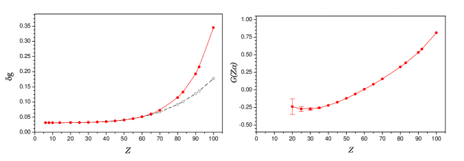
Figure 2: (Color online) The S(VP)E correction to the $1s$ bound-electron $g$ factor. Left graph presents our numerical all-order results (dots and solid line, red), together with the $Z\alpha$-expansion result (dashed line, black), in terms of $\delta g=\Delta g/(\alpha^{2}/\pi^{2})$. Right graph shows the corresponding results for the higher-order remainder $G(Z\alpha)$.

II Self-energy correction with vacuum-polarization insertion into the electron line

We now turn to the set of combined SE-and-VP diagrams depicted on Fig. 3, whose contribution will be referred to as the SEVP correction. This correction can be regarded as the one-loop SE correction to the $g$ factor, in which one of the bound-electron propagators is modified by the VP insertion. Since the VP insertion into the electron line can be represented by a local potential, the simplest way to calculate the SEVP correction is to redefine the bound-electron propagator by adding the VP potential to the binding nuclear potential. In this case, the SEVP correction can be obtained as a difference of the $g$ factor values with and without the VP addition in the binding potential.

The dominant part of the one-loop VP potential is given by the well-known Uehling potential:

$$V_{\rm Uehl}(r) = -Z\alpha\frac{2\alpha}{3\pi}\int\limits_{0}^{\infty}dr^{\prime}\;4\pi r^{\prime}\rho(r^{\prime})$$

$$\times\int\limits_{1}^{\infty}dt\;\left(1+\frac{1}{2t^{2}}\right)\frac{\sqrt{t^{2}-1}}{t^{2}}$$

$$\times\frac{e^{-2m|r-r^{\prime}|t}-e^{-2m(r+r^{\prime})t}}{4mrt}\,,$$

where $Z\rho(r)$ is the density of the nuclear charge distribution ($\int\rho(r)d{\bf r}=1$). The remaining part of the one-loop VP potential is given by the so-called Wichmann-Kroll potential $V_{\rm WK}$. For the purpose of the present investigation, it is sufficient to evaluate it by approximate formulas obtained in Ref. fainshtein:91 . The one-loop VP potential is then obtained as a sum of the Uehling and Wichmann-Kroll parts, $V_{\rm VP}(r)=V_{\rm Ueh}(r)+V_{\rm WK}(r)$.

In the present work, we calculate the SEVP correction by calculating the SE correction to the $g$ factor in the combined Coulomb and VP binding potential and subtracting the corresponding contribution evaluated with the Coulomb potential only. The result obtained in this way contains small additional contributions induced by second and higher-order iterations of the VP potential, but they may be disregarded at the present level of interest. The general scheme of calculation of the SE correction to the bound-electron $g$ factor was developed in our previous studies yerokhin:02:prl ; yerokhin:04 . In the present work, we extended this scheme for the case of the general binding potential. To this end, we employed the numerical approach for evaluation of the Dirac Green function for the arbitrary spherically symmetric potential (behaving as $\sim 1/r$ for $r\to\infty$) developed in Ref. yerokhin:11:fns .

Numerical results of our calculations of the SEVP correction for the $1s$ bound-state $g$ factor are presented in Table II. Our calculation was performed with the Fermi model of the nuclear charge distribution. The one-loop VP potential included both the Uehling and the Wichmann-Kroll contributions.

Comparison of our numerical results with the $Z\alpha$-expansion results is shown graphically on Fig. 4. The $Z\alpha$ expansion of the SEVP correction is given by pachucki:05:gfact

$$\Delta g_{\rm SEVP} \ =\left(\frac{\alpha}{\pi}\right)^{2}\,(Z\alpha)^{4}\,\biggl{[}\frac{4}{15}+(Z\alpha)\,G_{\rm SEVP}(Z\alpha)\biggr{]}\,,$$ (12)

where $G_{\rm SEVP}(Z\alpha)$ is the higher-order remainder. Note that the $Z\alpha$ expansion of the SEVP correction starts with the $(Z\alpha)^{4}$ term, so that the higher-order remainder is suppressed only by first power of $Z\alpha$ in this case.

The results of our calculations indicate that the higher-order contribution for the SEVP correction is remarkably large. Even for light systems like carbon and oxygen, the total correction is twice as large as the leading-order contribution, which is rather unusual. Notably, a large higher-order contribution stemming from the SEVP correction was previously reported also for the Lamb shift yerokhin:08:twoloop .

Figure 3: The combined self-energy and vacuum-polarization correction to the bound-electron $g$ factor with vacuum-polarization insertion into the electron line, referred to as the SEVP correction.

Table 2: The SEVP correction to the $1s$ bound-electron $g$ factor, in terms of $\delta^{(4)}g=\Delta g/[(\alpha^{2}/\pi^{2})(Z\alpha)^{4}]$.

$Z$	$\delta^{(4)}g$	$Z\alpha$-expansion
6	$0.62(2)$	$0.2667$
8	$0.736(3)$	$0.2667$
10	$0.845(2)$	$0.2667$
12	$0.948(2)$	$0.2667$
14	$1.045(1)$	$0.2667$
20	$1.310\,3(9)$	$0.2667$
24	$1.472\,5(8)$	$0.2667$
30	$1.702\,2(8)$	$0.2667$
32	$1.776\,7(4)$	$0.2667$
40	$2.074\,1(4)$	$0.2667$
50	$2.467\,8(2)$	$0.2667$
54	$2.640\,3(3)$	$0.2667$
60	$2.924\,3(2)$	$0.2667$
70	$3.486\,0(6)$	$0.2667$
80	$4.222\,3(6)$	$0.2667$
83	$4.488\,0(3)$	$0.2667$
90	$5.206\,1(7)$	$0.2667$
92	$5.429\,6(9)$	$0.2667$
100	$6.561(2)$	$0.2667$

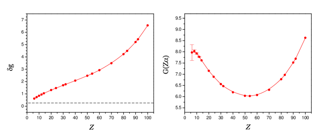
Figure 4: (Color online) SEVP correction to the $1s$ bound-electron $g$ factor. Left graph presents our numerical all-order results (dots and solid line, red), together with the $Z\alpha$-expansion result (dashed line, black), in terms of $\delta g=\Delta g/[(\alpha^{2}/\pi^{2})(Z\alpha)^{4}]$. Right graph shows the results for the higher-order remainder $G(Z\alpha)$.

III Two-loop vacuum-polarization correction

In this section we calculate the set of two-loop VP diagrams depicted in Fig. 5, referred to as the VPVP correction. The four diagrams in the set can be divided into two parts. The two diagrams on the left are induced by the second-order iteration of the one-loop VP potential, whereas the two diagrams on the right are induced by the two-loop VP potential. The complete form of the two-loop VP potential is not known at present. Its dominant part, however, is delivered by the free-loop approximation and is known for a long time, first derived by Källén and Sabry kaellen:55 . In the present work, we also treat the two-loop VP potential within the free-loop approximation only.

The VPVP contribution is given by the following expression

$$\Delta g_{\rm VPVP}= \ 2\,\langle\delta_{\rm VP}a|V_{\rm VP}|\delta_{g}a\rangle-2\,\langle a|V_{\rm VP}|a\rangle\,\langle\delta_{\rm VP}a|\delta_{g}a\rangle$$

$$+\langle\delta_{\rm VP}a|V_{g}|\delta_{\rm VP}a\rangle-\langle a|V_{g}|a\rangle\,\langle\delta_{\rm VP}a|\delta_{\rm VP}a\rangle$$

$$+2\,\langle a|V_{\rm KS}|\delta_{g}a\rangle\,,$$ (13)

where $|a\rangle$ is the reference-state wave function with a fixed momentum projection $\mu=1/2$, $|\delta_{\rm VP}a\rangle$ and $|\delta_{g}a\rangle$ are first-order perturbations of the reference-state wave function by the one-loop VP potential $V_{\rm VP}$ and the effective $g$-factor potential $V_{g}$,

$$|\delta_{\rm VP}a\rangle=\sum_{n\neq a}\frac{|n\rangle\langle n|V_{\rm VP}|a\rangle}{\varepsilon_{a}-\varepsilon_{n}}\,,$$ (14)

$$|\delta_{g}a\rangle=\sum_{n\neq a}\frac{|n\rangle\langle n|V_{g}|a\rangle}{\varepsilon_{a}-\varepsilon_{n}}\,,$$ (15)

the effective $g$-factor potential $V_{g}$ is

$$V_{g}=2m\,[\bm{r}\times\bm{\alpha}]_{z}\,,$$ (16)

and $V_{\rm KS}$ is the Källén-Sabry potential (see, e.g., Ref. fullerton:76 for explicit formulas). Note that the effective potential $V_{g}$ is defined so that its matrix element on the reference-state wave function with momentum projection $\mu=1/2$ is the Dirac value of the bound-electron $g$ factor, $\langle a|V_{g}|a\rangle=g_{D}$.

The numerical calculation of the VPVP correction is quite straightforward. It was performed by obtaining the perturbed wave functions with help of the dually kinetically balanced $B$-spline basis set method shabaev:04:DKB . Numerical results for the VPVP correction for the $1s$ bound-electron $g$ factor are presented in Table III. Comparison of our numerical all-order results with the $Z\alpha$ expansion results is given in Table III and graphically in Fig. 6. The $Z\alpha$ expansion of the VPVP correction reads

$$\Delta g_{\rm VPVP} \ =\left(\frac{\alpha}{\pi}\right)^{2}\,(Z\alpha)^{4}\,\biggl{[}-\frac{328}{81}+(Z\alpha)\,G_{\rm VPVP}(Z\alpha)\biggr{]}\,,$$ (17)

where $G_{\rm VPVP}(Z\alpha)$ is the higher-order remainder. The leading term of its $Z\alpha$ expansion was obtained previously in Ref. jentschura:09 , $G_{\rm VPVP}(Z\alpha)=7.4415187+O(Z\alpha)$.

We observe that our numerical all-order results agree well with the previous $Z\alpha$-expansion results. In particular, they confirm the conclusion of Ref. jentschura:09 that the higher-order VPVP contribution $G(Z\alpha)$ is rather large in the low-$Z$ region. In the high-$Z$ region, however, the large contribution of the $(Z\alpha)^{5}$ coefficient is compensated by higher-order terms, so that the total value of $G(Z\alpha)$ is significantly reduced and even changes its sign eventually as $Z$ increases.

Figure 5: The two-loop vacuum-polarization correction to the bound-electron $g$ factor (the VPVP correction).

Table 3: VPVP correction to the $1s$ bound-electron $g$ factor, in terms of $\delta^{(4)}g=\Delta g/[(\alpha^{2}/\pi^{2})(Z\alpha)^{4}]$.

$Z$	$\delta^{(4)}g$	$Z\alpha$-expansion
4	$-3.8556(1)$	$-3.83217$
6	$-3.7731(1)$	$-3.72356$
8	$-3.6983(1)$	$-3.61496$
10	$-3.6303(1)$	$-3.50635$
12	$-3.5686(1)$	$-3.39774$
14	$-3.5127(1)$	$-3.28914$
16	$-3.4619(1)$	$-3.18053$
18	$-3.4161(1)$	$-3.07192$
20	$-3.3749(1)$	$-2.96331$
24	$-3.3053(1)$	$-2.74610$
26	$-3.2765(1)$	$-2.63749$
28	$-3.2516(1)$	$-2.52889$
30	$-3.2303(1)$	$-2.42028$
32	$-3.2126(1)$	$-2.31167$
40	$-3.1771(1)$	$-1.87725$
50	$-3.2108(1)$	$-1.33421$
54	$-3.2502(1)$	$-1.11700$
60	$-3.3406(1)$	$-0.79118$
70	$-3.5857(1)$	$-0.24815$
80	$-3.9942(1)$	$0.29489$
83	$-4.1575(1)$	$0.45780$
90	$-4.6298(1)$	$0.83792$
92	$-4.7845(1)$	$0.94653$
100	$-5.6198(2)$	$1.38096$

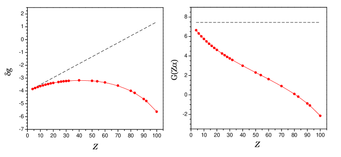
Figure 6: (Color online) VPVP correction to the $1s$ bound-electron $g$ factor. Left graph presents our numerical all-order results (dots and solid line, red), together with the $Z\alpha$-expansion results (dashed line, black), in terms of $\delta g=\Delta g/[(\alpha^{2}/\pi^{2})(Z\alpha)^{4}]$. Right graph shows the corresponding results for the higher-order remainder $G(Z\alpha)$.

IV Results and discussion

We now summarize our results obtained for the two-loop QED corrections with closed fermion loops. Since the previous investigations of these corrections have been performed within the $Z\alpha$ expansion and provided results complete up to order $\alpha^{2}\,(Z\alpha)^{4}$, we identify the higher-order remainder of our numerical results that can be directly added to the results obtained previously pachucki:05:gfact . The higher-order remainders induced by the three sets of two-loop diagrams with closed fermion loop considered in the present work are summarized in Table IV. We observe that the S(VP)E diagram yields a very small contribution to the higher-order remainder, whereas the remainders from the SEVP and VPVP diagrams are large and comparable in magnitude and enhance each other.

In Table IV, we collect all presently available contributions for the $1s$ bound-electron $g$ factor for four hydrogen-like ions that are most relevant from the experimental point of view. For three of them (carbon, oxygen, and silicon), accurate experimental results are already available haeffner:00:prl ; verdu:04 ; sturm:13:Si , whereas for calcium the experiment is underway blaum:priv . Since most of the results collected in Table IV appeared previously in the literature, we give here only short comments about the data presented in the table. The errors of the point-nucleus Dirac value and of the $(Z\alpha)^{0}$ part of the one-loop QED correction originate from the uncertainty of the fine-structure constant, $\alpha^{-1}=137.035\,999\,074(44)$ mohr:13:codata . The finite-nuclear-size correction is evaluated with the standard two-parameter Fermi model of the nuclear charge distribution and the root-mean-square radii taken from Ref. angeli:04 . The error of this correction originates both from the quoted uncertainty of the rms radius and from the dependence of the result on the model used for the nuclear-charge distribution.

The results obtained in the present work for the higher-order two-loop corrections with closed fermion loops are listed in the table under the labels ”$\geq$ 2-loop QED, h.o.” Since we did not calculate the complete two-loop QED correction in the present work (the two-loop self-energy contribution is left out), we do not decrease the overall uncertainty as compared to the previous investigations. Same as previously pachucki:05:gfact , the uncertainty due to higher-order two-loop contributions is estimated as

$$g^{(2)}_{\rm h.o.}=2\,g^{(1)}_{\rm h.o.}\,\frac{g^{(2)}[(Z\,\alpha)^{2}]}{g^{(1)}[(Z\,\alpha)^{2}]}\,,$$ (18)

where $g^{(n)}_{\rm h.o.}$ is the $n$-loop higher-order QED contribution and $g^{(n)}[(Z\,\alpha)^{2}]$ is the $n$-loop $(Z\,\alpha)^{2}$ QED contribution. We observe that the size of the two-loop contributions calculated in the present study is about 50% of the total uncertainty to the higher-order effects. So, we might refer to the size of the calculated effects as ”expected”.

Finally, we comment on the small differences (in the last significant digit) between the data in Table IV and the previous compilation in Ref. pachucki:05:gfact for the recoil corrections. The difference in the first-order ($\sim m/M$) recoil correction is due to the updated value of the nuclear masses, whereas the difference in the higher-order recoil correction is due to the updated theoretical result obtained in Ref. pachucki:08:recoil for the arbitrary nuclear spin.

It is interesting to note that the theoretical prediction for silicon reported in Table IV nearly coincides with the experimental result, leaving almost no space for the higher-order two-loop self-energy correction, which remains uncalculated at present. Indeed, the difference between theoretical and experimental results for Si amounts to $4\times 10^{-10}$, which is twice smaller than the two-loop contribution calculated in the present work. This indicates that either the two-loop self-energy contribution is relatively small or it changes its sign in the vicinity of $Z=14$. In order to test these assumptions, a $g$-factor measurement in a heavier system would be of great help. Table IV shows that already for calcium, the uncertainty due to the two-loop self-energy is by two orders of magnitude larger than the other theoretical errors. So, a measurement of the bound-electron $g$ factor in Ca¹⁹⁺ with the same accuracy as in Si would lead to an unambiguous experimental determination of the higher-order two-loop self-energy contribution.

Summarizing, we have calculated three sets of two-loop QED diagrams with the closed fermion loops to the $1s$ bound-electron $g$ factor. Calculations were performed to all orders in the nuclear binding strength parameter $Z\alpha$ except for the closed fermion loop, which was treated within the free-loop (Uehling) approximation in some cases. Our numerical data were shown to agree well with the $Z\alpha$-expansion results previously obtained for these corrections. The higher-order remainder [of order $\alpha^{2}(Z\alpha)^{5}$ and higher] was separated out from our numerical results. Its size agrees well with previous estimations for the two-loop higher-order effects. Our calculations do not improve the total uncertainty of the two-loop QED effects in the theoretical predictions since the most nontrivial two-loop correction, the two-loop self-energy, still remains to be calculated.

Acknowledgement

The work presented in the paper was supported by the Alliance Program of the Helmholtz Association (HA216/EMMI).

Table 4: The higher-order contribution to the $1s$ bound-electron $g$ factor induced by the two-loop QED diagrams with closed fermion loops, in terms of $\delta^{(5)}g=\Delta g/[(\alpha^{2}/\pi^{2})(Z\alpha)^{5}]$, where $\Delta g$ is the contribution to the $g$ factor.

$Z$	S(VP)E	SEVP	VPVP	$\delta^{(5)}g$	$\Delta g\times 10^{6}$
6	$0.00(15)^{a}$	$7.97(36)$	$6.31$	$14.28(39)$	$0.000\,012\,4(3)$
8	$-0.05(12)^{a}$	$8.03(6)$	$6.01$	$14.00(13)$	$0.000\,051\,2(5)$
14	$-0.15(4)^{a}$	$7.62(1)$	$5.25$	$12.72(4)$	$0.000\,764\,(3)$
20	$-0.23(2)^{a}$	$7.15(1)$	$4.62$	$11.54(2)$	$0.004\,12(1)$
30	$-0.27(2)$	$6.56$	$3.74$	$10.03(2)$	$0.027\,2(1)$
40	$-0.22$	$6.19$	$2.99$	$8.96$	$0.102\,4(1)$
50	$-0.12$	$6.03$	$2.30$	$8.21$	$0.286\,5(1)$
60	$0.01$	$6.07$	$1.62$	$7.70$	$0.668\,2(1)$
70	$0.16$	$6.30$	$0.91$	$7.37$	$1.382\,3(2)$
80	$0.33$	$6.78$	$0.09$	$7.20$	$2.632\,7(3)$
83	$0.38$	$6.97$	$-0.18$	$7.17$	$3.155\,0(3)$
90	$0.53$	$7.52$	$-0.88$	$7.17$	$4.726\,(1)$
92	$0.58$	$7.69$	$-1.10$	$7.18$	$5.281\,(1)$
100	$0.81$	$8.63$	$-2.15$	$7.28$	$8.134\,(3)$

^a extrapolated value.

Table 5: Individual contributions to the $1s$ bound-electron $g$ factor. The abbreviations used are as follows: “h.o.” stands for a higher-order contribution, “VP-EL” – for the electric-loop vacuum-polarization correction, “VP-ML” – for the magnetic-loop vacuum-polarization correction, “TW” indicates the results obtained in this work. $\langle r^{2}\rangle^{1/2}$ is the root-mean-square nuclear charge radius in fermi.

		${}^{12}{\rm C}^{5+}$	${}^{16}{\rm O}^{7+}$	${}^{28}{\rm Si}^{13+}$	${}^{40}{\rm Ca}^{19+}$	Ref.
$\langle r^{2}\rangle^{1/2}$		2.4703 (22)	2.7013 (55)	3.1223 (24)	3.4764 (10)
$m/M$		$4.5728\times 10^{-5}$	$3.4307\times 10^{-5}$	$1.9614\times 10^{-5}$	$1.3731\times 10^{-5}$
Dirac value (point)		$1.998\,721\,354\,39\,(1)$	$1.997\,726\,003\,06\,(2)$	$1.993\,023\,571\,6$	$1.985\,723\,203\,7\,(1)$
Finite nuclear size		$0.000\,000\,000\,41$	$0.000\,000\,001\,55\,(1)$	$0.000\,000\,020\,5$	$0.000\,000\,113\,0\,(1)$
1-loop QED	$(Z\,\alpha)^{0}$	$0.002\,322\,819\,47\,(1)$	$0.002\,322\,819\,47\,(1)$	$0.002\,322\,819\,5$	$0.002\,322\,819\,5$
	$(Z\,\alpha)^{2}$	$0.000\,000\,742\,16$	$0.000\,001\,319\,40$	$0.000\,004\,040\,6$	$0.000\,008\,246\,2$	grotch:70:prl
	$(Z\,\alpha)^{4}$	$0.000\,000\,093\,42$	$0.000\,000\,240\,07$	$0.000\,001\,244\,6$	$0.000\,002\,510\,6$	pachucki:04:prl
	h.o., SE	$0.000\,000\,008\,28$	$0.000\,000\,034\,43\,(1)$	$0.000\,000\,542\,8\,(3)$	$0.000\,003\,107\,7\,(2)$	yerokhin:02:prl ; pachucki:04:prl
	h.o., VP-EL	$0.000\,000\,000\,56$	$0.000\,000\,002\,24$	$0.000\,000\,032\,6$	$0.000\,000\,172\,7$	beier:00:rep
	h.o., VP-ML	$0.000\,000\,000\,04$	$0.000\,000\,000\,16$	$0.000\,000\,002\,5$	$0.000\,000\,014\,6$	lee:05
$\geq$2-loop QED	$(Z\,\alpha)^{0}$	$-0.000\,003\,515\,10$	$-0.000\,003\,515\,10$	$-0.000\,003\,515\,1$	$-0.000\,003\,515\,1$
	$(Z\,\alpha)^{2}$	$-0.000\,000\,001\,12$	$-0.000\,000\,002\,00$	$-0.000\,000\,006\,1$	$-0.000\,000\,012\,5$	grotch:70:prl
	$(Z\,\alpha)^{4}$	$0.000\,000\,000\,06$	$0.000\,000\,000\,08$	$-0.000\,000\,001\,3$	$-0.000\,000\,010\,9$	pachucki:05:gfact
	h.o.	$0.000\,000\,000\,01\,(3)$	$0.000\,000\,000\,05\,(11)$	$0.000\,000\,000\,8\,(17)$	$0.000\,000\,004\,1\,(100)$	TW
Recoil	$m/M$	$0.000\,000\,087\,73$	$0.000\,000\,117\,10$	$0.000\,000\,206\,1$	$0.000\,000\,297\,4$	shabaev:02:recprl
	h.o.	$-0.000\,000\,000\,10$	$-0.000\,000\,000\,13$	$-0.000\,000\,000\,2$	$-0.000\,000\,000\,3$	pachucki:08:recoil
Total		$2.001\,041\,590\,20\,(3)$	$2.000\,047\,020\,38\,(11)$	$1.995\,348\,958\,7\,(17)$	$1.988\,056\,950\,7\,(100)$
Experiment haeffner:00:prl ; verdu:04 ; sturm:13:Si		$2.001\,041\,596\,(5)$	$2.000\,047\,025\,4\,(46)$	$1.995\,348\,959\,10\,(81)$

Appendix A S(VP)E correction: zero-potential contribution

The zero-potential contribution of the S(VP)E correction can be derived by the method described in Ref. yerokhin:04 (Sec. IIIA) for the one-loop SE correction to the $g$ factor. Derivation requires explicit expressions for the free SE and vertex operators with the VP insertion into the photon line, which were obtained previously in Ref. yerokhin:08:pra (Sec. IIIC). The total zero-potential contribution of the S(VP)E correction to the $g$ factor is separated into three parts, which have the same meaning as in Ref. yerokhin:04 ,

$$\Delta g_{\rm vr}^{(0)}=\Delta g_{\rm ver,1}^{(0)}+\Delta g_{\rm ver,2}^{(0)}+\Delta g_{\rm red}^{(0)}\,.$$ (19)

The results for the three terms in the above equation are:

$$\Delta g_{\rm ver,1}^{(0)} \ =-\frac{\alpha^{2}}{4\pi^{5}}\,\int_{0}^{\infty}p_{r}^{2}dp_{r}\,\int_{0}^{1}dx\,dz\,\frac{z^{2}(1-z^{2}/3)}{1-z^{2}}\,\frac{1-x}{\Delta(\rho)}\,\biggl{[}g_{a}(\varepsilon_{a}g_{a}+p_{r}\,f_{a})-\frac{1}{3}f_{a}(\varepsilon_{a}f_{a}+p_{r}\,g_{a})\biggr{]}\,,$$ (20)

$$\Delta g_{\rm ver,2}^{(0)} \ =\frac{\alpha^{2}}{12\pi^{5}}\,\int_{0}^{\infty}p_{r}^{2}dp_{r}\,\int_{0}^{1}dx\,dz\,\frac{z^{2}(1-z^{2}/3)}{1-z^{2}}\,\frac{1-x}{\Delta(\rho)}\,$$

$$\times\biggl{\{}\Delta(\rho)\,\ln\frac{\Delta(\rho)}{\Delta(0)}\biggl{[}\frac{2}{p_{r}}\,g_{a}f_{a}+g_{a}f_{a}^{\prime}+f_{a}g_{a}^{\prime}\biggr{]}+2(1-x)(\varepsilon_{a}f_{a}+p_{r}\,g_{a})f_{a}-4f_{a}^{2}\biggr{\}}\,,$$ (21)

$$\Delta g_{\rm red}^{(0)} \ =g_{D}\,\frac{\alpha^{2}}{16\pi^{5}}\,\int_{0}^{\infty}p_{r}^{2}dp_{r}\,\int_{0}^{1}dx\,dz\,\frac{z^{2}(1-z^{2}/3)}{1-z^{2}}\,\frac{1-x}{\Delta(\rho)}\,$$

$$\times\biggl{\{}\Delta(\rho)\,\ln\frac{\Delta(\rho)}{\Delta(0)}(g_{a}^{2}+f_{a}^{2})-2\varepsilon_{a}(1-x)\biggl{[}\varepsilon_{a}(g_{a}^{2}+f_{a}^{2})+2p_{r}\,g_{a}f_{a}\biggr{]}+4\varepsilon_{a}\,(g_{a}^{2}-f_{a}^{2})\biggr{\}}\,,$$ (22)

where $\Delta(\rho)=x(1-\rho)+\rho+4(1-x)/[x(1-z^{2})]$, $\rho=(m^{2}-p^{2})/m^{2}=(m^{2}-\varepsilon_{a}^{2}+p_{r}^{2})/m^{2}$, $g_{D}$ is the lowest-order (Dirac) bound-electron $g$ factor, which for the $1s$ state is given by

$$g_{D}=\frac{2}{3}\left(1+2\,\sqrt{1-(Z\alpha)^{2}}\right)\,,$$ (23)

$\varepsilon_{a}$ is the reference-state energy, $g_{a}\equiv g_{a}(p_{r})$ and $f_{a}\equiv f_{a}(p_{r})$ are the upper and the lower components of the reference-state wave function in the momentum representation, respectively, and $g_{a}^{\prime}$ and $f_{a}^{\prime}$ denote derivatives of $g_{a}(p_{r})$ and $f_{a}(p_{r})$ with respect to $p_{r}$.

References

- (1) H. Häffner, T. Beier, N. Hermanspahn, H.-J. Kluge, W. Quint, S. Stahl, J. Verdú, and G. Werth, Phys. Rev. Lett. 85, 5308 (2000).
- (2) J. Verdú, S. Djekić, S. Stahl, T. Valenzuela, M. Vogel, G. Werth, T. Beier, H.-J. Kluge, and W. Quint, Phys. Rev. Lett. 92, 093002 (2004).
- (3) S. Sturm, A. Wagner, B. Schabinger, J. Zatorski, Z. Harman, W. Quint, G. Werth, C. H. Keitel, and K. Blaum, Phys. Rev. Lett. 107, 023002 (2011).
- (4) S. Sturm, A. Wagner, M. Kretzschmar, W. Quint, G. Werth, and K. Blaum, Phys. Rev. A 87, 030501 (2013).
- (5) A. Wagner, S. Sturm, F. Köhler, D. A. Glazov, A. V. Volotka, G. Plunien, W. Quint, G. Werth, V. M. Shabaev, and K. Blaum, Phys. Rev. Lett. 110, 033003 (2013).
- (6) V. A. Yerokhin, P. Indelicato, and V. M. Shabaev, Phys. Rev. Lett. 89, 143001 (2002).
- (7) V. M. Shabaev and V. A. Yerokhin, Phys. Rev. Lett. 88, 091801 (2002).
- (8) K. Pachucki, U. D. Jentschura, and V. A. Yerokhin, Phys. Rev. Lett. 93, 150401 (2004), [erratum: ibid., 94, 229902 (2005)].
- (9) K. Pachucki, A. Czarnecki, U. D. Jentschura, and V. A. Yerokhin, Phys. Rev. A 72, 022108 (2005).
- (10) Th. Beier, H. Häffner, N. Hermanspahn, S. G. Karshenboim, H.-J. Kluge, W. Quint, S. Stahl, J. Verdú, and G. Werth, Phys. Rev. Lett. 88, 011603 (2001).
- (11) P. J. Mohr, B. N. Taylor, and D. B. Newell, Rev. Mod. Phys. 84, 1527 (2012).
- (12) S. Sturm, A. Wagner, B. Schabinger, and K. Blaum, Phys. Rev. Lett. 107, 143003 (2011).
- (13) V. A. Yerokhin, P. Indelicato, and V. M. Shabaev, Phys. Rev. A 77, 062510 (2008).
- (14) V. A. Yerokhin, Phys. Rev. A 80, 040501(R) (2009).
- (15) V. A. Yerokhin, Eur. Phys. J. D 58, 57 (2010).
- (16) N. N. Bogoljubov and D. V. Shirkov, Introduction to the Theory of Quantized Fields, Interscience, New York, 1959.
- (17) S. Mallampalli and J. Sapirstein, Phys. Rev. A 54, 2714 (1996).
- (18) G. S. Adkins and J. Sapirstein, Phys. Rev. A 58, 3552 (1998).
- (19) V. A. Yerokhin, P. Indelicato, and V. M. Shabaev, Phys. Rev. A 69, 052503 (2004).
- (20) V. A. Yerokhin, Phys. Rev. A 78, 012513 (2008).
- (21) V. A. Yerokhin and V. M. Shabaev, Phys. Rev. A 64, 012506 (2001).
- (22) P. J. Mohr, Phys. Rev. Lett. 34, 1050 (1975).
- (23) A. G. Fainshtein, N. L. Manakov, and A. A. Nekipelov, J. Phys. B 24, 559 (1991).
- (24) V. A. Yerokhin, Phys. Rev. A 83, 012507 (2011).
- (25) G. Källen and A. Sabry, K. Dan. Vidensk. Selsk. Mat. Fys. Medd. 29 (1955).
- (26) L. W. Fullerton and J. G.A. Rinker, Phys. Rev. A 13, 1283 (1976).
- (27) V. M. Shabaev, I. I. Tupitsyn, V. A. Yerokhin, G. Plunien, and G. Soff, Phys. Rev. Lett. 93, 130405 (2004).
- (28) U. D. Jentschura, Phys. Rev. A 79, 044501 (2009).
- (29) P. J. Mohr and B. N. Taylor, Rev. Mod. Phys. 77, 1 (2005).
- (30) K. Blaum, priv. comm. (2013).
- (31) I. Angeli, At. Data Nucl. Data Tables 87, 185 (2004).
- (32) S. G. Karshenboim, Phys. Lett. A 266, 380 (2000).
- (33) T. Beier, Phys. Rep. 339, 79 (2000).
- (34) R. N. Lee, A. I. Milstein, I. S. Terekhov, and S. G. Karshenboim, Phys. Rev. A 71, 052501 (2005).
- (35) H. Grotch, Phys. Rev. Lett. 24, 39 (1970).
- (36) V. M. Shabaev, Phys. Rev. A 64, 052104 (2001).
- (37) H. Grotch, Phys. Rev. A 2, 1605 (1970).
- (38) R. Faustov, Phys. Lett. 33B, 422 (1970).
- (39) M. I. Eides and H. Grotch, Ann. Phys. (NY) 260, 191 (1997).
- (40) K. Pachucki, Phys. Rev. A 78, 012504 (2008).