Signatures Of Scalar Photon Interaction In Astrophysical Situations.

Abstract

Dimension-5 photon ($\gamma$) scalar ($\phi$) interaction term usually appear in the Lagrangians of bosonic sector of unified theories of electromagnetism and gravity. This interaction makes the medium dichoric and induces optical activity. Considering a toy model of an ultra-cold magnetized compact star ( White Dwarf (WD) or Neutron Star (NS)), we have modeled the propagation of very low energy photons with such interaction, in the environment of these stars. Assuming synchro-curvature process as the dominant mechanism of emission in such environments, we have tried to understand the polarimetric implications of photon-scalar coupling on the produced spectrum of the same. Further more assuming the ’emission-energy vs emission-altitude’ relation, that is believed to hold in such (i.e. cold magnetized WD or NS) environments, we have tried to point out the possible modifications to the radiation spectrum when the same is incorporated along with dim-5 photon scalar mixing operator.

PACS numbers: 14.80.Va, 87.19.lb, 95.30.Gv, 98.70.Vc
Key Words: Dimension-5 Scalar photon interaction, stokes parameters, compact stars.

1 Introduction.

Scalar $\phi(x)$ photon $\gamma$ interaction through dimension five operators originates in many theories beyond standard model of particle physics, usually in the unified theories of electromagnetism and gravity [1]. The scalars involved can be moduli fields of string theory, KK particles from extra dimension, scalar component of the gravitational multiplet in extended supergravity models etc. to name a few [​​ [2]-[9]].Though the main emphasis of such models had been unification of forces, however the same idea has also been used to solve the dark matter and dark energy [[10]–​​​[11]] problems of the universe, as in the chameleon models for dark matter[[12]–​​​[16]].

Physics of compactification–of extradimensions–introduces various kinds of model dependent interactions. For instance in the original Kaluza- Klein (KK) model [17], compactification of the extra fifth dimension was constructed to unify gravity with electromagnetism, that introduced dim-5 $\phi\gamma$ interaction. In string theories–constructed in ten or twenty six dimensions–the extra-dimensions are compactified and models have been made to find out various observable consequences of the same. One such model, invoked to explain the weakness of gravity relative to other forces, was developed by Arkani-Hamed, Dimopoulos and Dvali [18]. In this model, ( also known as “Large Extra Dimension” model), the standard model particles are confined to a four dimensional membrane, and gravity propagates in the other spatial dimensions, those are large compared to plank scale. However there also exist models ( with one or more extra spatial-dimensions ), where all fields propagate universally [19]. Collider signatures of Higher dimensions has been studied in [20]. Other than the collider signatures mentioned above, effort has also been made in [21], to relate the effect of extra dimension with four dimensional cosmological constant.

Interestingly enough, the dimension-5 photon scalar interaction term generated in the Lagrangian [17] by compactification of the extradimension, would eventually bear optical signatures of the same. The purpose of this note is to study such effects coming from dim-5 scalar photon interaction in some detail and shed some new light on their astrophysical consequences.
Usually dim-5 interactions (be it scalar photon or pseudoscalar (axion) photon interactions), induce optical activity. The scalar or pseudoscalar photon interaction turns vacuum into a birefringent and dichoric one [22, 23]. As a result, the plane of polarization of a plane polarized beam of light keeps on rotating as it passes through vacuum. This particular aspect of the theory has been exploited extensively in the literature in a different physical context (with pseudoscalar photon coupling) [[24]-[27]].

Keeping this in view, in this note, initially, we have studied the optical signatures of dim-5, $\phi F_{\mu\nu}F^{\mu\nu}$ interaction in an ambient magnetic field of strength $\sim 10^{13}$ Gauss. Following this, we have considered a toy model for the steller enviornment of a strongly magnetized, rotating, ultra cold, compact astrophysical objects like White Dwarf (WD) and Neutron Star (NS)–to understand some issues related to–emission energy and altitude [29], that is believed to affect the produced spectra of electromagnetic radiations (EM), originating there. As a next logical step, we have made an effort to explore the potential of the later, in modifying the usual spectral signatures of the tree-level dim-5, $\phi F_{\mu\nu}F^{\mu\nu}$ coupling–from such astrophysical situations. We would like to mention here, that, this model of ours is a toy model. The purpose of this construction is, to motivate further investigations of the possible modifications to the emission spectra, from actual WD or NS environment, when $\phi F_{\mu\nu}F^{\mu\nu}$ interaction has been taken into account.

While investigating the effects of $\phi F_{\mu\nu}F^{\mu\nu}$ interaction, in this note we have been able to achieve three objectives: (i) verifying the earlier results [23] through an independent approach, (ii) Showing the possibility of generation of circular and elliptic polarization from a plane polarized light beam–as the same passes through the steller environment.(iii) Pointing out the possibility of some extra modifications to the usual polarimetric signatures of $\phi F_{\mu\nu}F^{\mu\nu}$ coupling, due to emission altitude vs energy relation, that has been discussed in the literature [29].

It became very obvious for the first time in [28] that, existence of superluminal propagation modes for low frequency photons are possible, in a model with dimension-5 $\phi F_{\mu\nu}F^{\mu\nu}$ interaction term present in the Lagrangian. The analysis there, was performed in terms of the gauge potentials, using Lorentz gauge, leaving a scope of gauge ambiguities as a source of the problem. In order to rule out any role of the same, for the afore mentioned problem, we have taken a different approach, using the field strength tensors and Bianchi identity for deriving the same. Our new approach establishes the results obtained earlier.

To shed light on the second issue, we have assumed the radiation, produced at the production point, to be plane polarized electromagnetic wave ( with orthogonal planes of polarization, as is the case for synchro-curvature radiation). What we find is: the same generates a significant amount of scalar component through $\phi F_{\mu\nu}F^{\mu\nu}$ interaction, well before it is out of the stellar atmosphere ; this is some thing, that needs to be considered when one is looking for signatures of dim-5 mixing operators from astrophysical polarimetric data. Also, though the initial beam of radiation is plane polarized, however during its passage it picks up significant amount of elliptic/circular polarization through mixing. The amount of elliptic/circular polarization generated through mixing is energy $\omega$ dependent with a complex dependence on $\omega$ along with the strength of the magnetic field ${\cal{B}}$, coupling constant $g_{\gamma\gamma\phi}$ as well as the distance $z$ traveled in the stellar atmosphere. During our analysis, we have also looked into the pattern of polarization angle $\Psi$ and ellipticity angle $\chi$ that the beam of radiation generates at different wavelengths, after propagation through the same distance. What is very interesting is the existence of identical polarization angle ($\Psi$) at and ellipticity angle $\chi$ for multiple values of energies($\omega$) when the traversing path is same. The details of the same are discussed later.

The organization of the document is as follows, in section-II, we have derived the equations of motions. Section three is dedicated to the determination of the dispersion relations and the solutions of the equations of motions. In section four we discuss about the possible observables and applications, including a brief introduction to stokes parameters. Introduction to the physics of magnetized astrophysical compact objects ( toy model ) and ideas behind energy vs emission altitude mapping [​​[29]-[32]] is presented in section five. Results are presented in section VI. Lastly we conclude by pointing out the relevance of our analysis in realistic astrophysical or cosmological contexts.

2 From The Action To The Equations Of Motion.

To bring out the essential features of $\phi F_{\mu\nu}F^{\mu\nu}$ coupling term on the dynamics of the system, we would work in flat four dimensional space time. The action for this coupled scalar photon system in flat four dimensional space time is given by:

$$S\!=\!\!\int d^{4}x\!\left[\frac{1}{2}(\partial{{}_{\mu}})\phi(\partial^{\mu}\phi)-\frac{1}{4}g_{\phi\gamma\gamma}\phi F_{\mu\nu}F^{\mu\nu}-\frac{1}{4}F_{\mu\nu}F^{\mu\nu}\!\right]$$

(2.1)

Here $g_{\gamma\gamma\phi}$ is the effective coupling strength between scalar and electromagnetic field. The equations of motion can be obtained by varying the action with respect to $\phi$ and $F_{\mu\nu}$ and demanding invariance of the same under this arbitrary variation; the result is:,

$$\partial_{\mu}\left[F^{\mu\nu}+g_{\phi\gamma\gamma}\phi F^{\mu\nu}\right]=0$$

$$\partial_{\mu}\partial^{\mu}\phi+\frac{1}{4}g_{\phi\gamma\gamma}F_{\alpha\beta}F^{\alpha\beta}=0$$ (2.2)

As a next step we decompose the EM field into two parts, the mean field (${\bar{F}_{\mu\nu}}$) and the infinitesimal fluctuation ($f_{\mu\nu}$ ), i.e. :

$$F_{\mu\nu}={\bar{F}_{\mu\nu}}+f_{\mu\nu}.$$ (2.3)

Assuming the magnitude of the scalar field to be of the order of the fluctuating electromagnetic field $f_{\mu\nu}$ one can linearize the eqns in [2.2] . The equations of motions for the scalar and the electromagnetic fields turn out to be,

$$\partial_{\mu}f^{\mu\nu}=-g_{\phi\gamma\gamma}\partial_{\mu}\phi\bar{F}^{\mu\nu}.$$ (2.5)

$$\partial_{\mu}\partial^{\mu}\phi=-\frac{1}{2}g_{\phi\gamma\gamma}\bar{F}^{\mu\nu}f_{\mu\nu}$$ (2.6)

The two equations [2.5] and [2.6] are the two equations of motion governing the dynamics of the system in an external magnetic field described by the tensor $\bar{F}^{\mu\nu}$. Here we consider $\bar{F}^{\mu\nu}$ to be a very slowly varying function of coordinates, so that the same can be considered to be effectively constant. We note here that these two equations carry the information about the three degrees of freedom of the system, two for the two polarization states of the photon and the third one for the scalar degree of freedom.

3 Dispersion Relation.

In this section we would get the dispersion relation for the scalar photon coupled system of equations. Equation [2.5] in general would provide three equations, corresponding to two transverse and one longitudinal states of polarization for the photon. However in vacuum photons has only two transverse degrees of freedom, so one of the three would be redundant. The last equation i.e.,[2.6] would provide the dynamics of scalar degree of freedom, thus making the total number of degrees of freedom for the coupled system to be three.

We can get to the dynamics of the three degrees of freedom for the scalar photon system by two methods, by (a) using the gauge potentials and choosing a particular gauge, or by (b) making use of the Bianchi identity. In this work we would chose the second method. That is using the Bianchi identity:

$$\partial{{}_{\mu}}f_{\nu\lambda}+\partial{{}_{\nu}}f_{\lambda\mu}+\partial{{}_{\lambda}}f_{\mu\nu}=0.$$ (3.1)

If we now multiply the Bianchi Identity by $\bar{F}^{\nu\lambda}$ and operate with $\partial^{\mu}$, we arrive at the identity,

$$\partial_{\mu}\partial^{\mu}(f_{\lambda\rho}\bar{F}^{\lambda\rho})=-2\partial^{\lambda}\partial_{\mu}(f^{\mu\rho}\bar{F}_{\lambda\rho}).$$ (3.2)

One can now take equation, eqn.(2.5) and multiply it by $\bar{F}_{\nu\lambda}$ and operate with $\partial^{\lambda}$ subsequently use eqn. (3.2), to get to,

$$\partial_{\mu}\partial^{\mu}(\frac{f\bar{F}}{2})=g_{\phi\gamma\gamma}\partial^{\lambda}\partial_{\alpha}\phi(\bar{F}^{\alpha\nu}\bar{F}_{\nu\lambda})$$ (3.3)

Next we introduce a new variable, $\psi=f^{\nu\lambda}\bar{F}_{\nu\lambda}$, use it in eqn. (3.3) and go to momentum space. The resulting equation in momentum space is,

$$k^{2}\psi=g_{\phi\gamma\gamma}\left(k_{\alpha}\bar{F}^{\alpha\nu}\bar{F}_{\nu\lambda}k^{\lambda}\right)\phi$$ (3.4)

Similarly, defining, $\tilde{\psi}=f_{\mu\nu}\tilde{F}^{\mu\nu}$ and using same procedure one arrives at the equation for $\tilde{\psi}$. The same turns out to be,

$$k^{2}\tilde{\psi}=0$$ (3.5)

Finally the equation of motion for the scalar field in momentum space is given by,

$$k^{2}\phi=g_{\phi\gamma\gamma}\psi.$$ (3.6)

Assuming, $\bar{F}^{12}\neq 0$ therefore $\tilde{\bar{F}}^{03}\neq 0$ and denoting $\bar{F}^{12}=\cal{B}$, we may use the following compact representations for various Lorentz scalars e.g., $\left(\bar{F}^{\mu\nu}\bar{F}_{\mu\nu}\right)=2{\cal{B}}^{2},$ $\left(k_{\alpha}\bar{F}^{\alpha\nu}\bar{F}_{\nu\lambda}k^{\lambda}\right)=k^{2}_{\perp}{\cal{B}}^{2}$ and $\left(k_{\alpha}\tilde{\bar{F}}^{\alpha\nu}\tilde{\bar{F}}_{\nu\lambda}k^{\lambda}\right)=\left(k^{2}+k^{2}_{\perp}\right){\cal{B}}^{2}$ appearing in the equations of motion. In these expressions $k_{\perp}$ is the component of $\vec{K}$ that is orthogonal to ${\cal{B}}$ and $\Theta$ is the angle between the magnetic field B and the propagation direction $\vec{K}$. In terms of these we can rewrite the following expressions as:

$$k^{2}_{\perp}{\cal{B}}^{2}=K^{2}Sin^{2}(\Theta){\cal{B}}^{2} \simeq \omega^{2}Sin^{2}(\Theta){\cal{B}}^{2}$$

$$\left(k^{2}+k^{2}_{\perp}\right){\cal{B}}^{2}=\left(\omega^{2}-K^{2}Cos^{2}(\Theta)\right){\cal{B}}^{2} \simeq \left(\omega^{2}Sin^{2}(\Theta)\right){\cal{B}}^{2}.$$ (3.7)

While deriving the expressions in eqn. [3.7], we have assumed that, to order $g_{\gamma\gamma\phi}$, $\omega\simeq K$.

Being armed with these (i.e. findings of eqn. [3.7]), the equations of motions for the combined photon and scalar system can be written in matrix form:

$$\left(\begin{matrix}&k^{2}\,\,\,&0\,\,\,&0\cr&0\,\,\,&k^{2}\,\,\,&-g_{\phi\gamma\gamma}\omega^{2}Sin^{2}\Theta{\cal{B}}^{2}\cr&0\,\,\,&-g_{\phi\gamma\gamma}\,\,\,&k^{2}\end{matrix}\right)\left(\begin{matrix}{\tilde{\psi}}\cr\psi\cr\phi\end{matrix}\right)=0$$ (3.8)

The matrix equation [3.8] does not look symmetric because the dimension of $\phi$ and the dimensions of $\psi$ or $\tilde{\psi}$ are different. To bring the same in symmetric form, we multiply the $\phi$ equation in eqn.[3.6] by $\omega Sin\Theta{\cal{B}}$, and redefine $\phi$ by $\Phi$, when $\Phi=\omega Sin\Theta{\cal{B}}\phi$ to arrive at,

$$\left[\begin{matrix}&k^{2}&0&0\cr&0&k^{2}&-g_{\phi\gamma\gamma}\left(\omega Sin\Theta{\cal{B}}\right)\cr&0&-g_{\phi\gamma\gamma}\left(\omega Sin\Theta{\cal{B}}\right)&k^{2}\end{matrix}\right]\left[\begin{matrix}{\tilde{\psi}}\cr\psi\cr\Phi\end{matrix}\right]=0$$ (3.9)

3.1 Inhomogeneous Wave Equation.

It can be seen form eqn.[3.9], that because of the presence of off diagonal elements, two dynamical degrees of freedom out of the three, ( $\psi,~{}\tilde{\psi}$ and $\Phi$) during their propagation mix with each other. The matrix in eqn.[3.9] is real symmetric so we can go to a diagonal basis, by an orthogonal transformation to diagonalize the same. The orthogonal transformation matrix is given by,

$${\bf{O}}=\left(\begin{matrix}&1\,\,\,&0\,\,\,&0\cr&0\,\,\,&cos\theta\,\,\,&sin\theta\cr&0\,\,\,&-sin\theta\,\,\,&cos\theta\end{matrix}\right)\!,\rm{~{}where}~{}\theta=\frac{\pi}{4},\rm{~{}for~{}the~{}case~{}in~{}hand}.$$ (3.10)

On diagonalizing eqn. (3.9), we arrive at,

$$\left(\begin{matrix}&k^{2}\,\,\,&0\,\,\,&0\cr&0\,\,\,&k^{2}-g_{\gamma\gamma\phi}{\cal{B}}sin\Theta\omega\,\,\,&0\cr&0\,\,\,&0\,\,\,&k^{2}+g_{\gamma\gamma\phi}{\cal{B}}sin\Theta\omega\end{matrix}\right)\left(\begin{matrix}\tilde{\psi}\cr\frac{\Phi+\psi}{\sqrt{2}}\cr\frac{\Phi-\psi}{\sqrt{2}}\end{matrix}\right)=0$$ (3.11)

It is easy to see from the equation above that, $\tilde{\psi}$, $\frac{\psi+\Phi}{\sqrt{2}}$ and $\frac{-\psi+\Phi}{\sqrt{2}}$ satisfies the following dispersion relations,

$$\omega = K$$ (3.12)

$$\omega_{+} = \pm\sqrt{\left[K^{2}+g_{\gamma\gamma\phi}{\cal{B}}sin\Theta\omega\right]}$$ (3.13)

$$\omega_{-} = \pm\sqrt{\left[K^{2}-g_{\gamma\gamma\phi}{\cal{B}}sin\Theta\omega\right]}$$ (3.14)

Where, the quantity $g_{\gamma\gamma\phi}{\cal{B}}sin\Theta\omega$ depends on the strength of the external electromagnetic field, scalar photon coupling constant $g_{\phi\gamma\gamma}$, $\omega$ and the sine of the angle $\Theta$ between the direction of propagation $~{}\vec{K}~{}$ and the magnetic field ${\cal{B}}$.

It should be noted that equation [3.9] or [3.11], incorporates all the dispersive features of a photon propagating in a magnetized vacuum with dimension-five scalar photon interaction. One can verify that the dispersion relations obtained from [3.9] or [3.11] are identical to those in [23], provided appropriate limits are taken.

Its worth noting that eqn. [3.9] or [3.11] actually shows that in the case of scalar photon interaction, photons with polarization state perpendicular to the magnetic field ${\cal{B}}$ remains unaffected and propagates with speed of light and the same with polarization state parallel to the magnetic field couples to the scalar and undergoes modulation. As we will see later that there exists a critical energy ($\omega_{c}$) below of which the perpendicular modes have imaginary $\omega$, hence they would be non-propagating. However the perpendicular mode doesn’t suffer from this pathological problem, hence (for energy below $\omega_{c}$ ) they would propagate freely. Therefore light coming from distant sources with $\omega<\omega_{c}$ would appear to be linearly polarized provided this type of interaction does exist in nature.

We emphasize here, that, much of our analysis performed in this paper would have remained the same even if we had dim-5 pseudoscalar photon interaction, thus making it difficult to identify the type of interaction responsible for polarimetric observation that is being invoked in this note.

However, the way out is to note that the parallel and perpendicularly polarized components of the photon in these two different kind of interactions (scalar or pseudoscalar) interchange their role in presence of an external magnetic field. Hence the polarization state of the linearly polarized light for scalar photon interaction would be orthogonal to the same with Axion photon system. Therefore in principle one can look for this signature in polarimetric observations to point out the kind of interaction responsible for the type of signal.

3.2 Inhomogeneous Wave Equations.

The solutions for the dynamical degrees of freedom in coordinate space can be written as,

$$\left(\begin{matrix}\tilde{\psi}\cr cos\theta~{}\psi+sin\theta~{}\Phi\cr-sin\theta~{}\psi+cos\theta~{}\Phi\end{matrix}\right)=\left(\begin{matrix}A_{0}e^{i\left(\omega t-k.x\right)}\cr A_{1}e^{i\left(\omega_{+}t-k.x\right)}\cr A_{2}e^{i\left(\omega_{-}t-k.x\right)}\end{matrix}\right)$$ (3.15)

The constants, $A_{0},~{}A_{1}$  and $A_{2}$ has to be defined from the boundary conditions one imposes on the dynamical degrees of freedom. from eqn.[3.15] the solutions for the dynamical variables turn out to be,

$$\tilde{\psi}(t,x) = A_{0}\,\,e^{i\left(\omega t-k.x\right)}$$

$$\psi(t,x) = A_{1}\,\,cos\theta\,\,e^{i\left(\omega_{+}t-k.x\right)}-A_{2}\,\,sin\theta\,\,e^{i\left(\omega_{-}t-k.x\right)}$$ (3.16)

$$\Phi(t,x) = A_{1}\,\,sin\theta\,\,e^{i\left(\omega_{+}t-k.x\right)}+A_{2}\,\,cos\theta\,\,e^{i\left(\omega_{-}t-k.x\right)}.$$

In the following we consider the following boundary conditions, $\Phi(0,0)=0$ and $\psi(0,0)=1$. With this boundary condition we have, $\frac{A_{2}}{sin\theta}=-1$. And angle $\theta=\frac{\pi}{4}$ as has already been stated before. With these conditions the soln for $\psi$ turns out to be,

$$\psi(t,x)=\left[cos^{2}\theta\,\,e^{i\left(\omega_{+}t-k.x\right)}+sin^{2}\theta\,\,e^{i\left(\omega_{-}t-k.x\right)}\right].$$ (3.17)

Defining, $a^{2}_{x}(t)=\left({\rm{\cal{R}}}e\left[\psi(t,0)\right]\right)^{2}+\left(\rm{\cal{I}}m\left[\psi(t,0)\right]\right)^{2}$, we get the following the form for $\psi\left(t,x\right)$,

$$\psi(t,x)=a_{x}(t)e^{i\left(tan^{-1}\left[\frac{cos^{2}\theta\,\,sin\omega_{+}t+sin^{2}\theta\,\,sin\omega_{-}t}{cos^{2}\theta\,\,cos\omega_{+}t+sin^{2}\theta\,\,cos\omega_{-}t}\right]-kx\right)}$$ (3.18)

A wave equation of this type is usually called, inhomogeneous wave equation. The phase velocity for such system, where the solution is represented by, $a(t)e^{i\varphi(t)-kx}$ is defined by,

$$\mbox{{\cal{v}}}_{p}=\frac{1}{K}\frac{\partial\varphi(t)}{\partial t}$$ (3.19)

For the case under consideration, since $\theta=\frac{\pi}{4}$, the expression for the phase velocity can be evaluated exactly. It should be noted however, that, the same with nonzero scalar mass and/or other interactions present in the Lagrangian, may lead to a more complex situation and an exact analytical result may not be possible. We won’t be elaborating on this issue any further (here), it would be dealt with in a separate publication.

4 Application:

The predictions for the class of theories under consideration here, can be tested through optics based experiments set up for laboratory or astrophysical environments. For instance through the observations of the index of the power (of the ) spectrum, checking the differential dispersion measure or through the measurements of polarization angle, ellipticity at different wavelengths.

The analysis in this paper, are seemingly more suitable for dispersive and/or polarimetric measurements for verifying the predictions of these theories. More over, since we are more interested to find out the astrophysical implications of the theory being studied and optics based experiments are more suitable for the same, therefore, we will concentrate on dispersive or polarimetric analysis here.

4.1 Observables from non-thermal radiation.

In this section we would apply our results for astrophysical situations. They are of interest because the ambient magnetic field available there, are many orders of magnitude more, than the same available in laboratory conditions; also the length of the path the light beam traverses is enormous. Keeping this in view we would opt for astrophysical considerations. In astrophysical situations most of the interesting emission mechanisms are of no-thermal nature. As the charged particles in these situations accelerate in the ambient electromagnetic field, they radiate Electro Magnetic (EM) radiations.

4.2 Polarized spectrum.

In this section we provide the expression for the mutually orthogonal amplitudes of the polarized radiations coming from synchrotron or curvature radiations following [[33]- [35]].

The amplitudes of the electromagnetic radiation parallel or perpendicular to the $\hat{k}$ $\hat{B}$ plane–from the synchrotron or curvature radiation– are given by,

$$A_{\perp}\propto K_{1/3}\left(\frac{\omega}{2\omega_{sc}}\right)$$

$$A_{\parallel}\propto K_{2/3}\left(\frac{\omega}{2\omega_{sc}}\right)$$ (4.1)

In eqn.(4.1), $\omega_{sc}=\frac{3}{2}\frac{\Gamma^{3}}{\rho}$ is the peak energy for radiation spectrum with, $\Gamma$, the Lorentz boost factor for the emitting particles and $\rho$ the radius of curvature of the particle trajectory. The differential intensity spectrum, given by,

$$\frac{d^{2}I}{d\omega d\Omega}=\frac{(e\omega)^{2}}{4\pi^{2}}\left(|A_{\parallel}|^{2}+|A_{\perp}|^{2}\right),$$ (4.2)

grows as $\omega^{2/3}$ for $\omega\ll\omega_{sc}$, and falls off exponentially for $\omega\gg\omega_{sc}$. It is evident from eqn.(4.1) that, the EM spectrum from synchrotron or curvature radiation are emitted in two orthogonally polarized states.

4.3 Dispersive Measures

In astrophysical situations, dispersive and polarimetric measures are very effective to extract information about a system. For an object at a distance D we can measure the time taken by the signal to reach us by measuring $\frac{D}{v_{p}}$. That is, by measuring $t_{m}=\frac{D}{v_{p}}$ [36].

In cosmological situations red shift z can be, converted to proper distance using (for $\Omega=1$), $D=\frac{2}{3H_{0}}\left(1-\frac{1}{\left(1+z\right)^{3/2}}\right)$, with $H_{0}$ the Hubble constant being related to to h , by $h=\frac{H_{0}}{100\rm{~{}Sec}\rm{~{}Mpc}}km$ and $h=0.72\pm{0.05}$ obtained from the WMAP data [37]. Since we are using natural units, we can take $t=D$. This in principle can be performed for gamma-ray bursters or pulsar observations. In this energy band the dispersion measure of ( time ) should come out to be the proper provided restricts oneself to high energy band, to avoid the medium induced dispersion effects that’s dominant in the low energy domain.

In the previous sections we already have mentioned that, for the kind of interaction under consideration in this work, the vacuum turns out to be birefringent and dichoric for the photons. So the two polarized modes of photon, propagate with different speed. So, in principle, the orthogonally polarized signals from an astrophysical object, that originating from the source at the same space time point, would reach the observer at two different epochs. A similar argument taking into account the effect of stellar magnetized plasma was initially put forward in [38]-[41]. However,this argument has been discussed unfavorably in [42], and probably needs more refinement e.g., taking into account the kind of effect being discussed here and magnetized intergalactic domains, etc. Detailed analysis of this effect is beyond the scope of this paper and would be done elsewhere using the techniques of[43] .

4.4 Polarimetric measures

Most of the astrophysical objects are associated with magnetic field, with strengths varying from $10^{-9}$ to $10^{13}$ Gauss. Since synchrotron or curvature radiation are some of the most efficient non-thermal radiative mechanisms, the astrophysical objects mostly radiate non-thermally via this processes. A characteristic signature of the radiation coming through this process is, the radiation is polarized along and perpendicular to the $\hat{k}$, $\vec{\cal{B}}$ plane; where $\hat{k}$ is the direction vector from the source to the observer and $\hat{\cal{B}}$ is the ambient magnetic field direction. The amplitude and the spectrum of the radiation are well known and are discussed later in this paper.

The intrinsically polarized nature of the produced radiations turns out to be useful to perform polarimetric analysis of the observed data from astrophysical sources. The observables for polarimetric analysis are degrees of polarization, linear ($\Pi_{L}$)or circular ($\Pi_{c}$) and total polarization ($\Pi_{T}$) [44] . In view of this we would take a digression to the essentials of stokes parameters before estimating the polarimetric observables.

4.4.1 Digression on stokes parameters

In order to evaluate the polarimetric variables (Stokes parameters), one can construct the coherency matrix by taking different correlations of the vector potentials or the fields [44]. Various optical parameters of interest like polarization, ellipticity and degree of polarization of a given light beam, can be found from the components of the coherency matrix constructed from the correlation functions stated above [45].

For a little digression, the coherency matrix, for a system with two degree of freedom is defined as an ensemble average (where the averaging is done over many energy bands) of direct product of two vectors:

$$\rho(z)=\langle\left(\begin{matrix}\tilde{\psi}(z)\cr\psi(z)\end{matrix}\right)\otimes\left({\tilde{\psi}}(z)\,\,\,{\psi}(z)\right)^{*}\rangle=\left(\begin{matrix}\langle\tilde{\psi}(z)\tilde{\psi}^{*}(z)\rangle\,\,\,\langle\tilde{\psi}(z)\psi^{*}(z)\rangle\cr\langle\tilde{\psi}^{*}(z)\psi(z)\rangle\,\,\,\langle\psi(z)\psi^{*}(z)\rangle\end{matrix}\right)$$ (4.3)

One important thing to note here, is, under any anticlock-wise rotation by an angle $\alpha$ about an axis i.e., perpendicular to the vectors $\tilde{\psi}$ and $\psi$, the coherency matrix would transform as:

$$\rho(z)\to\rho^{\prime}(z)=\langle{\cal{R}}(\alpha)\left(\begin{matrix}{\tilde{\psi}}(z)\cr{\psi}(z)\end{matrix}\right)\otimes\left({\tilde{\psi}}(z)\,\,\,{\psi}(z)\right)^{*}{\cal{R}}^{-1}(\alpha)\rangle$$ (4.4)

where ${\cal{R}}(\alpha)$ is the rotation matrix. Now from the relations between the components of the coherency matrix and the stokes parameters:

$$\rm{I}\!\! = \!\!<\tilde{\psi}^{*}(z)\tilde{\psi}(z)>+<\psi^{*}(z)\psi(z)>,$$

$$\rm{Q}\!\! = \!\!<\tilde{\psi}^{*}(z)\tilde{\psi}(z)>-<\psi^{*}(z)\psi(z)>,$$

$$\rm{U}\!\! = \!\!2\rm{Re}<\tilde{\psi}^{*}(z)\psi(z)>,$$

$$\rm{V}\!\! = \!\!2\,\rm{Im}<\tilde{\psi}^{*}(z)\psi(z)>.$$ (4.5)

It is easy to establish that,

$$\rho(z)=\frac{1}{2}\left(\begin{matrix}{\rm{I}}(z)+~{}{\rm{Q}}(z)\,\,\,\,\,\,\,\,{\rm{U}}(z)-i{\rm{V}}(z)\cr{\rm{U}}(z)+i{\rm{V}}(z)\,\,\,\,\,\,{\rm{I}}(z)-~{}{\rm{Q}}(z)\end{matrix}\right)$$ (4.6)

Therefore, under an anticlock wise rotation by an angle $\alpha$, about an axis perpendicular to the plane containing $\tilde{\psi}(z)$ and $\psi(z)$, the density matrix transforms as: $\rho(z)~{}\to~{}\rho^{\prime}(z)$; hence the coherency matrix in the rotated frame would be given by,

$$\rho^{\prime}(z) = \frac{1}{2}{\cal{R}}(\alpha)\left(\begin{matrix}{\rm{I}}(z)+~{}{\rm{Q}}(z)\,\,\,\,\,\,\,\,{\rm{U}}(z)-i{\rm{V}}(z)\cr{\rm{U}}(z)+i{\rm{V}}(z)\,\,\,\,\,\,{\rm{I}}(z)-~{}{\rm{Q}}(z)\end{matrix}\right){\cal{R}}^{-1}(\alpha)~{}.$$ (4.7)

Since for a rotation by an angle $\alpha$–in the anticlock wise direction ( about the axis that is perpendicular to the plane having $\tilde{\psi}$ and $\psi$ on it ) the rotation matrix ${\cal{R}}(\alpha)$ is given by,

$${\cal{R}}(\alpha)=\left(\begin{matrix}{\rm{cos}}~{}{\alpha}\,\,\,\,\,\,\,\,{\rm{sin}}~{}{\alpha}\cr-{\rm{sin}}~{}{\alpha}\,\,\,\,\,\,\,\,{\rm{cos}}~{}{\alpha}\end{matrix}\right),$$ (4.8)

as a consequence the two stokes parameters $Q^{\prime}$(z) and $U^{\prime}$ (z), in the rotated frame of reference, would get related to the same in the unrotated frame, by the relation.

$$\left(\begin{matrix}{\rm{Q}}^{{}^{\prime}}(z)\cr{\rm{U}}^{{}^{\prime}}(z)\end{matrix}\right)=\left(\begin{matrix}{\rm{cos}}~{}{2\alpha}\,\,\,\,\,\,\,\,{\rm{sin}}~{}{2\alpha}\cr-{\rm{sin}}~{}{2\alpha}\,\,\,\,\,\,\,\,{\rm{cos}}~{}{2\alpha}\end{matrix}\right)\left(\begin{matrix}{\rm{Q}}(z)\cr{\rm{U}}(z)\end{matrix}\right)$$ (4.9)

The other two parameters, i.e., I and V remain unaltered. It is for this reason that some times I and V are termed invariants under rotation.

We would like to point out here that, in any frame, the Stokes parameters are expressed in terms of two angular variables $\chi$ and $\Psi$ usually called the ellipticity parameter and polarization angle, defined as,

$${\rm{I}} = {\rm{I}}_{p}$$

$${\rm{Q}} = {\rm{I}}_{p}{\rm{cos}}~{}2\Psi~{}{\rm{cos}}~{}2\chi$$

$${\rm{U}} = {\rm{I}}_{p}{\rm{sin}}~{}2\Psi~{}{\rm{cos}}~{}2\chi$$

$${\rm{V}} = {\rm{I}}_{p}{\rm{sin}}~{}2\chi.$$ (4.10)

The ellipticity angle, $\chi$, following [4.10], can be shown to be equal to,

$${\rm{tan}}2\chi=\frac{{\rm{V}}}{\sqrt{{\rm{Q}^{2}}+{\rm{U}}^{2}}}~{},$$ (4.11)

and the polarization angle can be shown to be equal to.

$${\rm{tan}}2\Psi=\frac{\rm{U}}{\rm{Q}}$$ (4.12)

From the relations given above, it is easy to see that, under the frame rotation,

$${\cal{R}}(\alpha)=\left(\begin{matrix}{\rm{cos}}~{}{2\alpha}\,\,\,\,\,\,\,\,{\rm{sin}}~{}{2\alpha}\cr-{\rm{sin}}~{}{2\alpha}\,\,\,\,\,\,\,\,{\rm{cos}}~{}{2\alpha}\end{matrix}\right)$$ (4.13)

the Tangent of $\chi$, i.e., ${\rm{tan}}\chi$ remains invariant, however the tangent of the polarization angle gets additional increment by twice the rotation angle, i.e.,

$${\rm{tan}}(2\chi) \to{\rm{tan}}(2\chi)$$

$${\rm{tan}}(2\Psi) \to{\rm{tan}}(2\alpha+2\Psi).$$ (4.14)

It is worth noting that the two angles are not quite independent of each other, in fact they are related to each other. Finally we end the discussion of use of stokes parameters by noting that, the degree of polarization is usually expressed by,

$$p=\frac{\sqrt{{\rm{Q}}^{2}+{\rm{U}}^{2}+{\rm{V}}^{2}}}{{\rm{I}}_{P_{T}}}$$ (4.15)

where ${\rm{I}}_{P_{T}}$ is the total intensity of the light beam.

Since we already have the expressions for the stokes parameters in terms of the solutions of the field equations (3.2) one can substitute the solutions of the field equations in (4.5) to arrive at the expressions for $I$, $Q$, $U$ and $V$. The expressions for the same are given by,

$$I(\omega,z) = \frac{1}{2}\left[3+cos\left[\left(\omega_{-}-\omega_{+}\right)z\right]\right]$$ (4.16)

$$Q(\omega,z) = \frac{1}{2}\left[cos\left[\left(\omega_{-}-\omega_{+}\right)z\right]-1\right]$$ (4.17)

$$U(\omega,z) = 2.0\left[cos\left[\left(\frac{\omega_{+}-\omega_{-}}{2}\right)z\right]\right]\left[cos\left[\left(\frac{\omega_{+}-\omega_{-}}{2}-\omega\right)z\right]\right]$$ (4.18)

$$V(\omega,z) = -2\left[cos\left[\left(\frac{\omega_{+}-\omega_{-}}{2}\right)z\right]\right]\left[sin\left[\left(\frac{\omega_{+}-\omega_{-}}{2}+\omega\right)z\right]\right]$$ (4.19)

5 Astrophysical Accelerators

Standard astrophysical accelerators of charged particles in our universe are, white dwarf (WD) pulsar, neutron star (NS) pulsars, supernova remnants (SNRs), micro-quasars and possibly gamma-ray bursters [[46]-[68]] to name a few. As the charged particles accelerate along the dipole magnetic field lines [69] of these astrophysical accelerators, they emit energy through synchro-curvature radiation [[70] -[72]], whose spectrum (in familiar notations), peaks at $\omega_{sc}=\frac{3\Gamma^{3}}{2\rho}$ .

For our analysis we would dealing with the emission spectra and polarization studies of compact stars e.g., white dwarf pulsar or neutron star pulsars. We will be following the analysis of [[70] -[72]] and [[73] [74]] in this paper. According to the rotating dipole model [69] of compact stars, a strong electric field of magnitude, $E_{\parallel}=\frac{\vec{E}.\vec{\cal{B}}}{|\vec{{\cal{B}}}|}$ is generated along the magnetic field in the co-rotating magnetosphere of the pulsar. This can accelerate particles to ultra high energies [75]. During their accelerating phase the charged particles emit EM radiation through synchro-curvature radiation to be detected by a faraway observer [​​[69]–[77]].

A relativistic charged particle of mass m, if moves through a distance $ds$, in this electric field, then the change in its energy ( in natural units ), can be written as:

$$d\left(\Gamma m\right)=\vec{E}_{\parallel}.\vec{ds}=-\vec{\nabla}\left(eV\right).\vec{ds}.$$ (5.1)

where $V$ is the scalar potential. The solution of the same in one dimension is provides the value of $\Gamma$ (Lorentz Boost) as a function of position. It comes out to be:

$$\Gamma(s)=-\frac{eV(s)}{m}+\rm{constant},$$ (5.2)

where the distance s is measured from the center of the star. The value of the constant is fixed by assuming that on the surface of the compact object, velocity of the charged particle was zero, and at the surface of the star parallel component of the electric field vanishes, hence, one arrives finally at:

$$\Gamma(s)=1-\frac{eV(s)}{m}.$$ (5.3)

Equation (5.3), is the same as reported in [77]. The unity in eqn. (5.3) is usually neglected for large Lorentz boost [73], however for consistency it has to be retained. Using the relation $V(r)=-\int^{r}_{0}E_{\parallel}.ds$( when $R$ is the radius of the star), one can find out the value of $\Gamma(r)$ for a particular position $r$. According to polar cap model, a compact star with surface magnetic field ${\cal{B}}_{s}$, angular velocity $\Omega=\frac{2\pi}{P}$ (when P is the period), would have electric field $E_{\parallel}$, close to the star surface, given by $E_{\parallel}\simeq\frac{{\cal{B}}_{s}}{192}\left(\frac{\Omega R}{c}\right)^{\frac{5}{2}}\frac{s}{\Delta R_{p}}$ for $0\leq s\leq\Delta R_{p}$ [[73], [76]]. The Polar cap radius is denoted by, $\Delta R_{p}\simeq\sqrt{\left[\frac{\Omega R}{c}\right]}R$, with $c$ as the velocity of light and is equal to unity according to our system of units. This relation makes it is easy to observe that, the value of the Lorentz boost at a hight $r=\alpha\Delta R_{p}(0\leq\alpha\leq 1.)$ from the surface of the star is:

$$\Gamma(r)=\frac{1}{16\sqrt{3}}\left(\Omega R\right)^{3}\left(\frac{e{\cal{B}}}{m}\right)R\alpha^{2}$$ (5.4)

when the distance $r=\alpha\left(\Delta R_{P}\right)$, i.e., a fraction of the polar cap radius from the surface of the star. One can combine this result with the expression for $\omega_{sc}$, to get a relation between emission energy vs hight.

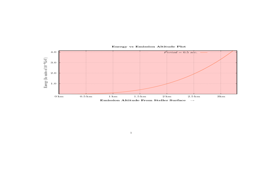
Figure 1: Plot Of Emission altitude versus energy of emitted synchrotron radiation, for a relatively cold compact star (white dwarf) with dipolar magnetic field strength $\sim 10^{13}$, Gauss and period 0.5 sec.

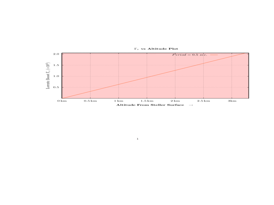
Figure 2: Plot of Lorentz boost of charged fermions emitting synchrotron radiation versus emission altitude, for a relatively cold compact star, with same field strength and spin period as in Figure 3.

Normally astrophysical compact stars, White Dwarfs (WD) or Neutron Stars (NS ) appear with surface magnetic field strength varying between $10^{9}$ -$10^{13}$ Gauss. The surface dipolar magnetic field strength for young pulsars are more ($<10^{9}$ Gauss) than the older ones($>10^{9}$ Gauss). Assuming the surface dipolar magnetic field strength to be around critical magnetic field, i.e $4.4\times 10^{13}$ Gauss and a period of 0.5 sec, we have plotted the distance vs boost as well as synchrotron emission energy $\omega_{sc}$ in Fig. [2] and Fig. [2] respectively. As can be seen form the plots, that, for a compact star of radius 10 km or $10^{6}$cm, the synchro-curvature radiation reaches the value of $10^{-8}$GeV, within 2 km hight from the surface of the star. The same keeps on increasing as one moves further away from the surface of the star.

There are two relevant points worth mentioning here, (i) with increase in the time period $P$ of the compact object, energy of the emitted radiation at a fixed altitude would tend to increase (ii) we would be assuming that the photon emission process, takes place close to the last open field line and it’s quasi tangential to the surface of the star. Although the magnetic field strength is expected to vary as ${\cal{B}}(r)=\frac{{\cal{B}}_{S}(R)R^{2}}{r^{2}}$ (a condition that follows from the flux conservation), but because of the special emission geometry we have assumed, the observables, like $\Psi,\chi$ etc., would not undergo significant variation because of the variation of the ambient magnetic field.

6 Result and Analysis

Earlier we have shown that, the curvature radiation amplitudes for the plane polarized photons in the magnetized stellar environment follows from eqn. [4.1]. Since our objective in this work to bring out salient features of such emission, therefore we have assumed the initial amplitudes of the two orthogonal polarized modes to be of same magnitude. Though this is a simplified assumption, to be true for modeling of realistic emission processes taking place in compact astrophysical objects (WD or NS), however, as it will be clear below, that this is sufficient to bring out the new physics issues, those we wish to focus on.

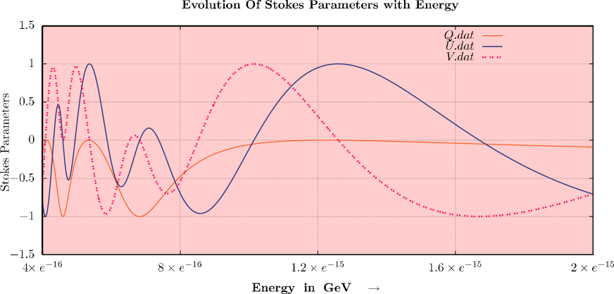
Figure 3: Plots for Stokes parameters, Q (orange line), U (blue line) and V (dotted orange line), for coupling constant $g_{\gamma\gamma\phi}\!=\!10^{-11}GeV^{-1}$ and ${\cal{B}}=4.41\times 10^{13}$ Gauss–vs $\omega$.

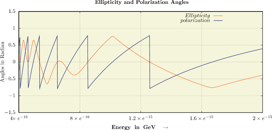
Figure 4: Plots for polarization angle $\Psi$ (blue line) and ellipticity $\chi$ (orange line), for coupling constant $g_{\gamma\gamma\phi}\!=\!10^{-11}GeV^{-1}$ and ${\cal{B}}=4.41\times 10^{13}$ Gauss–vs $\omega$.

The physics of the optical activity, in this scenario, is the following, as the produced electromagnetic beam propagates in the magnetized stellar environment, the photons with polarization orthogonal to the magnetic field, keep mixing with the scalars resulting in a change of phase for the same; and the photons with polarization along the magnetic field propagates freely. The superposition of the two decides the net polarization of the system. Since the change of phase is dependent on (a) the path traversed by the radiation beam, (b) the strength of the ambient magnetic field and (c) the frequency of the photons– the final magnitude of the net polarization of the radiation beam depends on all the three.

Since we are interested in the wave propagation in an ambient ( magnetic ) field of strength $\sim 10^{13}$ Gauss, believed to exist close to surface of the star, we need know the critical synchro-curvature energy $\omega_{sc}$, of the emitted photons there in.
The same has been obtained, as already mentioned, using the relations of section IV. The critical energy of the emitted photons, as a function of altitude from a ultra cold, (WD or NS) pulsar ( with period P=0.5 sec.) was evaluated and plotted in Fig. [2]. The numerical data showed that, at altitudes very close to the surface of the star ( $\leq 0.1$ km), the critical energy, turns out to be of the order of $O(10^{-16})$ GeV, and it reaches the value of $O(10^{-8})$ GeV, at an altitude of $3.5$ km or so.
Therefore assuming the initial amplitudes for both the polarized modes to be the same, we have estimated the stokes parameters numerically for a frequency range of $4.0\times 10^{-16}$ GeV to $2.0\times 10^{-15}$ GeV, for $g_{\gamma\gamma c}=\left(10^{11}GeV\right)^{-1}$ (from PVLAS data [79] ) and magnetic field strength ${\cal{B}}=4.41\times 10^{13}$ Gauss. The propagation length is taken to be about $5\times 10^{5}$ cm ( about $\frac{R_{s}}{10}$, when $R_{s}=10^{6}$cm, is the stellar radius which is close to that of the astrophysical compact objects). The result is plotted in the Fig. [4].

As can be verified from the initial conditions that, at $z=0$ the stokes parameter U is nonzero but Q and V are both zero ( i.e we have linearly polarized light ). However the variations of the same, after propagation through, a distance $\frac{R_{s}}{10}$, as a function of energy $\omega$ can be seen from figure . As is clear from the plots, that at low energy, elliptic polarization, defined by Stokes parameter V, though is small in magnitude but the same undergoes modulation with increasing $\omega$. Similar behavior is also observed to be taking place with U. However, the Stokes parameter Q doesn’t undergo similar modulation in magnitude at high energies.
It can be checked from the plots that there are situations when both Q and V are simultaneously zero except U, signaling linear polarization and vice-verse. As the frequency changes, the degree of linear polarization decreases and that of circular polarization increases. This is due to $\gamma$, $\phi$ mixing effect. We would like to emphasize here that, degree of linear and circular polarization due to $\phi F_{\mu\nu}F^{\mu\nu}$ coupling need not be of very close order at all energies.

The other important observation that we had mentioned already is, that the ellipticity $\chi$ and polarization angles $\Psi$ are generally multi-valued functions of the energy $\omega$. There can be various values of energies $\omega$ at which the $\Psi$ and $\chi$ could turn out to be the same, but mostly they are not, as can be seen from Fig. 4.
It should however be noted that, the effects we have discussed so far are purely due to mixing, where the polarized multi wavelength beams are supposed to have travelled the same distance. This may be achievable in laboratory conditions, however,the same may not hold for all class of astrophysical objects and all kinds of emissions mechanisms.

Compact astrophysical objects (stars) usually radiates through synchro-curvature radiation, in many energy bands. Energy of an emitted photon depends on the emission altitude–measured from the surface of the star. For compact stars, this relationship, is referred at times as altitude energy mapping. The nature of this mapping depends on the details of the model of the compact object. In our illustrative model the low energy photons originate close to and higher energy photons originate far away from the surface of the compact star. Therefore the low energy modes would pass through larger distance in the magnetized media than the high energy ones.
So the kind of polarizations two light beams ( say at two different energies $\omega_{1}$ and $\omega_{2}$, with $\omega_{1}<\omega_{2}$), are going to acquire would be different once they are out of the stellar environment. This is because the two different path lengths traveled by the the two beams in the magnetized stellar media, due to emission geometry. Since for the kind of physical picture for we have in mind ( WD, NS or Quasars ), a radiation beam, due to altitude energy effect ( following dipole emission models ), would be having multiple energies where each of these individual components would be traveling different path-lengths in the magnetized stellar atmosphere, once out of the stellar environment. Therefore, in addition to the $\gamma\phi$ mixing induced polarization effects–an additional path dependent effect would also show up at various energy bands of the synchro-curvature radiations coming from WD or NS because emission-altitude energy relations, that these radiations follow. Hence, for a consistent interpretation of the observations, the same needs to be accounted for.

6.0.1 Modified Boundary Conditions For Scalars.

Another important point that we would like to point out here, is, although the number of scalar particles produced in the synchro-curvature emission model of WD or NS are usually zero ( from kinematical or other considerations ), however, by the time the emitted radiation is out of the stellar environment a significant amount of scalars may be generated because of the mixing effect.
Therefore, while analyzing synchro-curvature spectra of radiations from far away WD or NS, one would need to take this in to consideration for the fixing boundary conditions, along with the effect of multiple magnetized intergalactic domains ( similar model was considered in [78], however the radiation sources considered there were different).

7 Discussion and Outlook.

In this section we briefly summarize the findings of this work. We have tried to point out, in this work, the important polarimetric signatures in the synchro- curvature radiation spectra of cosmologically far away compact objects (WD or NS) because of scalar photon mixing.

Our findings are the following: the mixing effect itself is capable of producing (a) Elliptic or Circular polarization from initially Plane Polarized beams, (b) the amount of or plane, circular or elliptic polarization generated at different energies need not be of same magnitude at all energy bands, for the beams traveling through the same distance and same fields strength ( magnetic field strength ${\cal{B}}$), (c) Polarization and Ellipticity angles are multivalued functions of energy. There may be several energy bands where the angles repeat themselves, (d) significant amount of scalars may be produced in the beams once they are out of the stellar environment, (e) the physics of emission of synchro-curvature radiation for these sources, makes the monochromatic beams at different energy bands, travel different path lengths in the stellar environment. Hence a phase difference, coming from the difference of path travelled by the beams of light at different $\omega$, will contribute to their polarimetric signatures. Therefore, even with running the risk of repetition, we would like to emphasize, that, degree of linear and circular polarization need not be close to each other, with dim-5 photon scalar coupling.

Once the electromagnetic signal is out of the stellar environment, it would propagate through the ambient magnetized intersteller, galactic and inter-galactic space before reaching the observer. Signals from far away objects may also travel through multiple magnetized domains in the inter-galactic space. Since EM waves undeergo Faraday Rotation [80] in magnetized enviornment, therefore to find out the contribution of scalar photon mixing operator to polarimetric data, one needs to estimate further, the Faraday rotation induced contribution to the same, following the procedure discussed in [81]. However, this analysis is out of scope of current study and the same will be undertaken else where.