Min-Max Design of FIR Digital Filters by Semidefinite Programming

Abstract.

In this article we consider two problems: FIR (Finite Impulse Response) approximation of IIR (Infinite Impulse Response) filters and inverse FIR filtering of FIR or IIR filters. By means of Kalman-Yakubovich-Popov (KYP) lemma and its generalization (GKYP), the problems are reduced to semidefinite programming described in linear matrix inequalities (LMIs). MATLAB codes for these design methods are given. An design example shows the effectiveness of these methods.

1. Introduction

Robustness is a fundamental issue in signal processing; unmodeled dynamics and unexpected noise in systems and signals are inevitable in designing systems and signals. Against such uncertainties, min-max optimization, or worst case optimization is a powerful tool. In this light, we propose an efficient design method of FIR (finite impulse response) digital filters for approximating and inverting given digital filters. The design is formulated by min-max optimization in the frequency domain. More precisely, we design an FIR filter which minimizes the maximum gain of the frequency response of an error system.

This design has a direct relation with $H^{\infty}$ optimization [1]. Since the space $H^{\infty}$ is not a Hilbert space, the familiar projection method cannot be applied. However, many studies have been made on the $H^{\infty}$ optimization, and nowadays the optimal solution to the $H^{\infty}$ problem is deeply analysed and can be easily obtained by numerical computation. Moreover, as an extension of $H^{\infty}$ optimization, a min-max optimization on a finite frequency interval has been proposed recently [2]. In both optimization, the Kalman-Yakubovich-Popov (KYP) lemma [3, 4, 5] and the (generalized) KYP lemma [2] give an easy and fast way of numerical computation; semidefinite programming [6]. Semidefinite programming can be efficiently solved by numerical optimization softwares.

In this article, we consider two fundamental problems of signal processing: FIR approximation of IIR (infinite impulse response) filters and inverse FIR filtering of FIR/IIR filters. Each problems are formulated in two types of optimization: $H^{\infty}$ optimization and finite-frequency min-max one. These problems are reduced to semidefinite programming in a similar way. For this, we introduce state-space representation. Semidefinite programming is obtained by the generalized KYP lemma. We will give MATLAB codes for the proposed design, and will show design examples.

2. Preliminaries

In this article, we frequently use notations in control systems. For readers who are not familiar to these, we here recall basic notations and facts of control systems used throughout the article. We also show MATLAB codes for better understanding.

Let us begin with a linear system ${\mathcal{G}}$ represented in the following state-space equation or state-space representation [7]:

(1) $${\mathcal{G}}:\left\{~{}~{}\begin{split}x[k+1]&=Ax[k]+Bu[k],\\ y[k]&=Cx[k]+Du[k],~{}~{}k=0,1,2,\ldots.\end{split}\right.$$

The nonnegative number $k$ denotes the time index. The vector $x[k]\in{\mathbb{R}}^{n}$ is called the state vector, $u[k]\in{\mathbb{R}}$ is the input and $y[k]\in{\mathbb{R}}$ is the output of the system ${\mathcal{G}}$. The matrices $A\in{\mathbb{R}}^{n\times n}$, $B\in{\mathbb{R}}^{n\times 1}$, $C\in{\mathbb{R}}^{1\times n}$, and $D\in{\mathbb{R}}$ are assumed to be static, that is, independent of the time index $k$. Then the transfer function $G(z)$ of the system ${\mathcal{G}}$ is defined by

$$G(z):=C(zI-A)^{-1}B+D.$$

The transfer function $G(z)$ is a rational function of $z$ of the form

(2) $$G(z)=\frac{b_{n}z^{n}+b_{n-1}z^{n-1}+\cdots+b_{1}z+b_{0}}{z^{n}+a_{n-1}z^{n-1}+\cdots+a_{1}z+a_{0}}.$$

Note that $G(z)$ is the $Z$-transform of the impulse response $\{g[k]\}_{k=0}^{\infty}$ of the system ${\mathcal{G}}$ with the initial state $x[0]=0$, that is,

$$G(z)=\sum_{k=0}^{\infty}g[k]z^{-k}=D+\sum_{k=1}^{\infty}CA^{k-1}Bz^{-k}.$$

To convert a state-space equation to its transfer function, one can use the above equations or the MATLAB command tf. On the other hand, to convert a transfer function to a state-space equation, one can use realization theory which provides methods to derive the state space matrices from a given transfer function [7]. An easy way to obtain the matrices is to use MATLAB or Scilab with the command ss.

Example 1.

We here show an example of MATLAB commands. First, we define state-space matrices:

>A=[0,1;-1,-2]; B=[0;1]; C=[1,1]; D=0;
>G=ss(A,B,C,D,1);

This defines a state-space (ss) representation of ${\mathcal{G}}$ with the state-space matrices

$$A=\begin{bmatrix}0&1\\ -1&-2\end{bmatrix},~{}B=\begin{bmatrix}0\\ 1\end{bmatrix},~{}C=\begin{bmatrix}1&1\end{bmatrix},~{}D=0.$$

The last argument 1 of ss sets the sampling period to be 1.

To obtain the transfer function $G(z)=C(zI-A)^{-1}B+D$, we can use the command tf

>> tf(G)

Transfer function:
    z + 1
-------------
z^2 + 2 z + 1

Sampling time (seconds): 1

On the other hand, suppose that we have a transfer function at first:

>> z=tf(’z’,1);
>> Gz=(z^2+2*z+1)/(z^2+0.5*z+1);

The first command defines the variable $z$ of $Z$-transform with sampling period 1, and the second command defines the following transfer function:

$$G(z)=\frac{z^{2}+2z+1}{z^{2}+0.5z+1}.$$

To convert this to state-space matrices $A$, $B$, $C$, and $D$, use the command ss as follows:

>> ss(Gz)

a =
         x1    x2
   x1  -0.5    -1
   x2     1     0

b =
       u1
   x1   1
   x2   0

c =
        x1   x2
   y1  1.5    0

d =
       u1
   y1   1

Sampling time (seconds): 1
Discrete-time model.

These outputs shows that the state-space matrices are given by

$$A=\begin{bmatrix}-0.5&-1\\ 1&0\end{bmatrix},~{}B=\begin{bmatrix}1\\ 0\end{bmatrix},~{}C=\begin{bmatrix}1.5&0\end{bmatrix},~{}D=1,$$

with sampling time 1. $\Box$

Note that the state-space representation in Example 1 is minimal in that the state-space model describes the same input/output behavior with the minimum number of states. Such a system is called minimal realization [7].

We then introduce a useful notation, called packed notation [8], describing the transfer function from state-space matrices as

$$G(z)=C(zI-A)^{-1}B+D=:\left[\begin{array}[]{c|c}A&B\\ \hline\cr C&D\end{array}\right]\!(z).$$

By the packed notation, the following formulae are often used in this article:

(10) $$\left[\begin{array}[]{c|c}A_{1}&B_{1}\\ \hline\cr C_{1}&D_{1}\end{array}\right]\times\left[\begin{array}[]{c|c}A_{2}&B_{2}\\ \hline\cr C_{2}&D_{2}\end{array}\right] =\left[\begin{array}[]{cc|c}A_{2}&0&B_{2}\\ B_{1}C_{2}&A_{1}&B_{1}D_{2}\\ \hline\cr D_{1}C_{2}&C_{1}&D_{1}D_{2}\\ \end{array}\right],$$

(18) $$\left[\begin{array}[]{c|c}A_{1}&B_{1}\\ \hline\cr C_{1}&D_{1}\end{array}\right]\pm\left[\begin{array}[]{c|c}A_{2}&B_{2}\\ \hline\cr C_{2}&D_{2}\end{array}\right] =\left[\begin{array}[]{cc|c}A_{1}&0&B_{1}\\ 0&A_{2}&\pm B_{2}\\ \hline\cr C_{1}&C_{2}&D_{1}\pm D_{2}\\ \end{array}\right].$$

Next, we define stability of linear systems. The state-space system ${\mathcal{G}}$ in (1) is said to be stable if the eigenvalues $\lambda_{1},\ldots,\lambda_{n}$ of the matrix $A$ lie in the open unit circle ${\mathbb{D}}=\left\{z\in{\mathbb{C}}:\left|z\right|<1\right\}$. Assume that the transfer function $G(z)$ is irreducible. Then ${\mathcal{G}}$ is stable if and only if the poles of the transfer function $G(z)$ lie in ${\mathbb{D}}$. To compute the eigenvalues of $A$ in MATLAB, use the command eig(A), and for the poles of $G(z)$ use pole(Gz).

The $H^{\infty}$ norm is the fundamental tool in this article. The $H^{\infty}$ norm of a stable transfer function $G(z)$ is defined by

$$\|G\|_{\infty}:=\max_{\omega\in[0,\pi]}\left|G(e^{j\omega})\right|.$$

This is the maximum gain of the frequency response $G(e^{j\omega})$ of ${\mathcal{G}}$ as shown in Fig. 1.

Figure 1. The $H^{\infty}$ norm $\|G\|_{\infty}$ of $G(z)$ is the maximum value of the frequency response gain $\left|G(e^{j\omega})\right|$.

The MATLAB code to compute the $H^{\infty}$ norm of a transfer function is given as follows:

>> z=tf(’z’,1);
>> Gz=(z-1)/(z^2-0.5*z);
>> norm(Gz,inf)

ans =

    1.3333

This result shows that for the stable transfer function

$$G(z)=\frac{z-1}{z^{2}-0.5z},$$

the $H^{\infty}$ norm is given by $\|G\|_{\infty}\approx 1.3333$.

$H^{\infty}$ control or $H^{\infty}$ optimization is thus minimization of the maximum value of a transfer function. This leads to robustness against uncertainty in the frequency domain. Moreover, it is known that the $H^{\infty}$ norm of a transfer function $G(z)$ is equivalent to the $\ell^{2}$-induced norm of ${\mathcal{G}}$, that is,

$$\|G\|_{\infty}=\|{\mathcal{G}}\|:=\sup_{\begin{subarray}{c}u\in\ell^{2}\\ u\neq 0\end{subarray}}\frac{\|{\mathcal{G}}u\|_{2}}{\|u\|_{2}},$$

where $\|u\|_{2}$ is the $\ell^{2}$ norm of $u$:

$$\|u\|_{2}:=\left(\sum_{n=0}^{\infty}\left|u[k]\right|^{2}\right)^{1/2}.$$

The $H^{\infty}$ norm optimization is minimization of the system gain when the worst case input is applied. This fact implies that the $H^{\infty}$ norm optimization leads to robustness against uncertainty in input signals.

3. $H^{\infty}$ Design Problems of FIR Digital Filters

In this section, we consider two fundamental problems in signal processing: filter approximation and inverse filtering. The problems are formulated as $H^{\infty}$ optimization by using the $H^{\infty}$ norm mentioned in the previous section.

3.1. FIR approximation of IIR filters

The first problem we consider is approximation. In signal processing, there are a number of design methods for IIR (infinite impulse response) filters, e.g., Butterworth, Chebyshev, Elliptic, and so on [9]. In general, to achieve a given characteristic, IIR filters require fewer memory elements, i.e., $z^{-1}$, than FIR (finite impulse response) filters. However, IIR filters may have a problem of instability since they have feedbacks in their circuits, and hence, we prefer an FIR filter to an IIR one in implementation. For this reason, we employ FIR approximation of a given IIR filter. This problem has been widely studied [9]. Many of them are formulated by $H^{2}$ optimization; they aim at minimizing the average error between a given IIR filter and the FIR filter to be designed. This optimal filter works well averagely, but in the worst case, the filter may lead a large error. To guarantee the worst case performance, $H^{\infty}$ optimization is applied to this problem [10]. The problem is formulated as follows:

Problem 1 (FIR approximation of IIR filters).

Given an IIR filter $P(z)$, find an FIR (finite impulse response) filter $Q(z)$ which minimizes

$$\left\|(P-Q)W\right\|_{\infty}=\max_{\omega\in[0,\pi]}\left|\left(P(e^{j\omega})-Q(e^{j\omega})\right)W(e^{j\omega})\right|,$$

where $W$ is a given stable weighting function.

The procedure to solve this problem is shown in Section 4.

3.2. Inverse filtering

Inverse filtering, or deconvolution is another fundamental issue in signal processing. This problem arises for example in direct-filter design in spline interpolation [11].

Suppose a filter $P(z)$ is given. Symbolically, the inverse filter of $P(z)$ is $P(z)^{-1}$. However, real design is not that easy.

Example 2.

Suppose $P(z)$ is given by

$$P(z)=\frac{z+0.5}{z-0.5}.$$

Then, the inverse $Q(z):=P(z)^{-1}$ becomes

$$Q(z)=P(z)^{-1}=\frac{z-0.5}{z+0.5},$$

which is stable and causal. Then suppose

$$P(z)=\frac{z-2}{z-0.5},$$

then the inverse is

$$Q(z)=P(z)^{-1}=\frac{z-0.5}{z-2}.$$

This has the pole at $\left|z\right|>1$, and hence the inverse filter is unstable. On the other hand, suppose

$$P(z)=\frac{1}{z-0.5},$$

then the inverse is

$$Q(z)=P(z)^{-1}=z-0.5,$$

which is noncausal.

By these examples, the inverse filter $P(z)^{-1}$ may unstable or noncausal. Unstable or noncausal filters are difficult to implement in real digital device, and hence we adopt approximation technique; we design an FIR digital filter $Q(z)$ such that $Q(z)P(z)\approx 1$. Since FIR filters are always stable and causal, this is a realistic way to design an inverse filter. Our problem is now formulated as follows:

Problem 2 (Inverse filtering).

Given a filter $P(z)$ which is necessarily not bi-stable or bi-causal (i.e., $P(z)^{-1}$ can be unstable or noncausal), find an FIR filter $Q(z)$ which minimizes

$$\left\|(QP-1)W\right\|_{\infty}=\max_{\omega\in[0,\pi]}\left|\left(Q(e^{j\omega})P(e^{j\omega})-1\right)W(e^{j\omega})\right|,$$

where $W$ is a given stable weighting function.

The procedure to solve this problem is shown in Section 4.

4. KYP Lemma for $H^{\infty}$ Design Problems

In this section, we show that the $H^{\infty}$ design problems given in the previous section are efficiently solved via semidefinite programming [6]. For this purpose, we first formulate the problems in state-space representation reviewed in Section 2. Then we bring in Kalman-Yakubovich-Popov (KYP) lemma [3, 4, 5] to reduce the problems into semidefinite programming.

4.1. State-space representation

The transfer functions $\left(P(z)-Q(z)\right)W(z)$ and $\left(Q(z)P(z)-1\right)W(z)$ in Problems 1 and 2, respectively, can be described in a form of

(19) $$T(z)=T_{1}(z)+Q(z)T_{2}(z),$$

where

$$T_{1}(z)=P(z)W(z),\quad T_{2}(z)=-W(z),$$

for Problem 1 and

$$T_{1}(z)=-W(z),\quad T_{2}(z)=P(z)W(z),$$

for Problem 2. Therefore, our problems are described by the following min-max optimization:

(20) $$\min_{Q(z)\in{\mathcal{F}}_{N}}\|T_{1}+QT_{2}\|_{\infty}=\min_{Q(z)\in{\mathcal{F}}_{N}}\max_{\omega\in[0,\pi]}\left|T_{1}(e^{j\omega})+Q(e^{j\omega})T_{2}(e^{j\omega})\right|,$$

where ${\mathcal{F}}_{N}$ is the set of $N$-th order FIR filters, that is,

$${\mathcal{F}}_{N}:=\left\{Q(z):Q(z)=\sum_{i=0}^{N}\alpha_{i}z^{-i},\alpha_{i}\in{\mathbb{R}}\right\}.$$

To reduce the problem of minimizing (20) to semidefinite programming, we use state-space representation for $T_{1}(z)$ and $T_{2}(z)$ in (19). Let $\{A_{i},B_{i},C_{i},D_{i}\}$ $(i=1,2)$ are state-space matrices of $T_{i}(z)$ in (19), that is,

$$T_{i}(z)=C_{i}(zI-A_{i})^{-1}B_{i}+D_{i}=:\left[\begin{array}[]{c|c}A_{i}&B_{i}\\ \hline\cr C_{i}&D_{i}\end{array}\right],\quad i=1,2.$$

Also, a state-space representation of an FIR filter $Q(z)$ is given by

(21) $$Q(z)=\sum_{n=0}^{N}\alpha_{n}z^{-n}=\left[\begin{array}[]{ccccc|c}0&1&0&\ldots&0&0\\ 0&0&1&\ddots&\vdots&\vdots\\ 0&0&\ddots&\ddots&0&\vdots\\ \vdots&\vdots&\ddots&0&1&0\\ 0&0&\ldots&0&0&1\\ \hline\cr\alpha_{N}&\alpha_{N-1}&\ldots&\alpha_{2}&\alpha_{1}&\alpha_{0}\\ \end{array}\right]\!(z)=:\left[\begin{array}[]{c|c}A_{q}&B_{q}\\ \hline\cr\alpha_{N:1}&\alpha_{0}\end{array}\right]\!(z),$$

where $\alpha_{N:1}:=\left[\begin{array}[]{ccccc}\alpha_{N}&\alpha_{N-1}&\ldots&\alpha_{1}\end{array}\right]$.

By using these state-space matrices, we obtain a state-space representation of $T(z)$ in (19) as

(22) $$T(z)=\left[\begin{array}[]{ccc|c}A_{1}&0&0&B_{1}\\ 0&A_{2}&0&B_{2}\\ 0&B_{q}C_{2}&A_{q}&B_{q}D_{2}\\ \hline\cr C_{1}&\alpha_{0}C_{2}&\alpha_{N:1}&D_{1}+\alpha_{0}D_{2}\end{array}\right]\!(z)=:\left[\begin{array}[]{c|c}A&B\\ \hline\cr C(\alpha_{N:0})&D(\alpha_{0})\end{array}\right]\!(z).$$

Note that the FIR parameters $\alpha_{0},\alpha_{1},\ldots,\alpha_{N}$ depend affinely on $C$ and $D$, and are independent of $A$ and $B$. This property is a key to describe our problem into semidefinite programming.

4.2. Semidefinite programming by KYP lemma

The optimization in (20) can be equivalently described by the following minimization problem:

$$\text{minimize }\gamma\text{ subject to }Q(z)\in{\mathcal{F}}_{N}\text{ and}$$

(23) $$\max_{\omega\in[0,\pi]}\left|T_{1}(e^{j\omega})+Q(e^{j\omega})T_{2}(e^{j\omega})\right|\leq\gamma.$$

To describe this optimization in semidefinite programming, we adopt the following lemma [3, 4, 5]:

Lemma 1 (KYP lemma).

Suppose

$$T(z)=\left[\begin{array}[]{c|c}A&B\\ \hline\cr C&D\end{array}\right]\!(z)$$

is stable, and the state-space representation $\{A,B,C,D\}$ of $T(z)$ is minimal. Let $\gamma>0$. Then the following are equivalent conditions:

1. $\|T\|_{\infty}\leq\gamma$.

2. There exists a positive definite matrix $X$ such that

   $$\begin{bmatrix}A^{\top}XA-X&A^{\top}XB&C^{\top}\\ B^{\top}XA&B^{\top}XB-\gamma^{2}&D\\ C&D&-1\end{bmatrix}\leq 0.$$

By using this lemma, we obtain the following theorem:

Theorem 1.

The inequality (23) holds if and only if there exists $X>0$ such that

(24) $$\begin{bmatrix}A^{\top}XA-X&A^{\top}XB&C(\alpha_{N:0})^{\top}\\ B^{\top}XA&B^{\top}XB-\gamma^{2}&D(\alpha_{0})\\ C(\alpha_{N:0})&D(\alpha_{0})&-1\end{bmatrix}\leq 0,$$

where $A$, $B$, $C(\alpha_{N:0})$, and $D(\alpha_{0})$ are given in (22).

By this, the optimal FIR parameters $\alpha_{0},\alpha_{1},\ldots,\alpha_{N}$ can be obtained as follows. Let $x$ be the vector consisting of all variables in $\alpha_{N:0}$, $X$, and $\gamma^{2}$ in (24). The matrix in (24) is affine with respect to these variables, and hence, can be rewritten in the form

$$M(x)=M_{0}+\sum_{i=1}^{L}M_{i}x_{i},$$

where $M_{i}$ is a symmetric matrix and $x_{i}$ is the $i$-th entry of $x$. Let $v\in\{0,1\}^{L}$ be a vector such that $v^{\top}x=\gamma^{2}$. Our problem is then described by semidefinite programming as follows:

$$\text{minimize }v^{\top}x\text{ subject to }M(x)\leq 0.$$

By this, we can effectively approach the optimal parameters $\alpha_{N:0}$ by numerical optimization softwares. For MATLAB codes of the semidefinite programming above, see Section 7.

5. Finite Frequency Design of FIR Digital Filters

By the $H^{\infty}$ design discussed in the previous section, we can guarantee the maximum gain of the frequency response of $T=(P-Q)W$ (approximation) or $T=(QP-1)W$ (inversion) over the whole frequency range $[0,\pi]$. Some applications, however, do not need minimize the gain over the whole range $[0,\pi]$, but a finite frequency range $\Omega\subset[0,\pi]$. Design of noise shaping $\Delta\Sigma$ modulators is one example of such requirement [12]. In this section, we consider such optimization, called finite frequency optimization. We first consider the approximation problem over a finite frequency range.

Problem 3 (Finite frequency approximation).

Given a filter $P(z)$ and a finite frequency range $\Omega\subset[0,\pi]$, find an FIR filter $Q(z)$ which minimizes

$$V_{\Omega}(P-Q):=\max_{\omega\in\Omega}\left|P\left(e^{j\omega}\right)-Q\left(e^{j\omega}\right)\right|.$$

Figure 2. Finite frequency approximation (Problem 3): the error gain $\left|P\left(e^{j\omega}\right)-Q\left(e^{j\omega}\right)\right|$ is minimized over the finite frequency range $\Omega_{\mathrm{low}}=[0,\omega_{\mathrm{low}}]$.

Figure 2 illustrates the above problem for a finite frequency range $\Omega=\Omega_{\mathrm{low}}=[0,\omega_{\mathrm{low}}]$, where $\omega_{\mathrm{low}}\in(0,\pi]$. We seek an FIR filter which minimizes $V_{\Omega}(P-Q)$ over the finite frequency range $\Omega$, and do not care about the other range $[0,\pi]\setminus\Omega$. We can also formulate the inversion problem over a finite frequency range.

Problem 4 (Finite frequency inversion).

Given a filter $P(z)$ and a finite frequency range $\Omega\subset[0,\pi]$, find an FIR filter $Q(z)$ which minimizes

$$V_{\Omega}(QP-1):=\max_{\omega\in\Omega}\left|Q(e^{j\omega})P(e^{j\omega})-1\right|.$$

These problems are also fundamental in digital signal processing. We will show in the next section that these problems can be also described in semidefinite programming via generalized KYP lemma.

6. Generalized KYP Lemma for Finite Frequency Design Problems

In this section, we reduce the problems given in the previous section to semidefinite programming. As in the $H^{\infty}$ optimization, we first formulate the problems in state-space representation, and then derive semidefinite programming via generalized KYP lemma [2].

6.1. State-space representation

As in the $H^{\infty}$ optimization in Section 4, we employ state-space representation. Let $T(z)=P(z)-Q(z)$ for the approximation problem or $T(z)=P(z)Q(z)-1$ for the inversion problem. Then $T(z)$ can be described by $T(z)=T_{1}(z)+Q(z)T_{2}(z)$ as in (19). Then our problems are described by the following min-max optimization:

(25) $$\min_{Q(z)\in{\mathcal{F}}_{N}}V_{\Omega}\left(T_{1}+QT_{2}\right)=\min_{Q(z)\in{\mathcal{F}}_{N}}\max_{\omega\in\Omega}\left|T_{1}(e^{j\omega})+Q(e^{j\omega})T_{2}(e^{j\omega})\right|.$$

Let $\{A_{i},B_{i},C_{i},D_{i}\}$, $i=1,2$ be state-space matrices of $T_{i}(z)$. By using the same technique as in Section 4, we can obtain a state-space representation of $T(z)$ as

(26) $$T(z)=\left[\begin{array}[]{c|c}A&B\\ \hline\cr C(\alpha_{N:0})&D(\alpha_{0})\end{array}\right]\!(z),$$

where $\alpha_{N:0}=[\alpha_{N},\ldots,\alpha_{0}]$ is the coefficient vector of the FIR filter to be designed as defined in (21).

6.2. Semidefinite programming by generalized KYP lemma

The optimization in (25) can be equivalently described by the following problem:

$$\text{minimize }\gamma\text{ subject to }Q(z)\in{\mathcal{F}}_{N}\text{ and}$$

(27) $$\max_{\omega\in[0,\pi]}\left|T_{1}(e^{j\omega})+Q(e^{j\omega})T_{2}(e^{j\omega})\right|\leq\gamma$$

To describe this optimization in semidefinite programming, we adopt the following lemma [2]:

Lemma 2 (Generalized KYP Lemma).

Suppose

$$T(z)=\left[\begin{array}[]{c|c}A&B\\ \hline\cr C&D\end{array}\right]\!(z)$$

is stable, and the state-space representation $\{A,B,C,D\}$ of $T(z)$ is minimal. Let $\Omega$ be a closed interval $[\omega_{1},\omega_{2}]\subset[0,\pi]$. Let $\gamma>0$. Then the following are equivalent conditions:

1. $V_{\Omega}(T)=\max_{\omega\in[\omega_{1},\omega_{2}]}\left|T\left(e^{j\omega}\right)\right|\leq\gamma$.

2. There exist symmetric matrices $Y>0$ and $X$ such that

   $$\left[\begin{array}[]{ccc}M_{1}(X,Y)&M_{2}(X,Y)&C^{\top}\\ \overline{M}_{2}(X,Y)^{\top}&M_{3}(X,\gamma^{2})&D\\ C&D&-1\\ \end{array}\right]\leq 0,$$

   where

   (28) $$\begin{split}M_{1}(X,Y)&=A^{\top}XA+YAe^{-j\omega_{0}}+A^{\top}Ye^{j\omega_{0}}-X-2Y\cos r,\\ M_{2}(X,Y)&=A^{\top}XB+YBe^{-j\omega_{0}},\quad\overline{M}_{2}(X,Y)=A^{\top}XB+YBe^{j\omega_{0}},\\ M_{3}(X,\gamma^{2})&=B^{\top}XB-\gamma^{2},\quad\omega_{0}=\frac{\omega_{1}+\omega_{2}}{2},\quad r=\frac{\omega_{2}-\omega_{1}}{2}.\end{split}$$

By using this lemma, we obtain the following theorem:

Theorem 2.

The inequality (27) holds if and only if there exist symmetric matrices $Y>0$ and $X$ such that

$$\left[\begin{array}[]{ccc}M_{1}(X,Y)&M_{2}(X,Y)&C(\alpha_{N:0})^{\top}\\ \overline{M}_{2}(X,Y)^{\top}&M_{3}(X,\gamma^{2})&D({\alpha_{0}})\\ C(\alpha_{N:0})&D(\alpha_{0})&-1\\ \end{array}\right]\leq 0,$$

where $M_{1}$, $M_{2}$, and $M_{3}$ are given in (28), $A$, $B$, $C(\alpha_{N:0})$, and $D(\alpha_{0})$ are given in (26).

By this theorem, we can obtain the coefficients $\alpha_{0},\ldots,\alpha_{N}$ of the optimal FIR filter by semidefinite programming as mentioned in Section 4. MATLAB codes for the semidefinite programming are shown in Section 7.

7. MATLAB Codes for Semidefinite Programming

In this section, we give MATLAB codes for the semidefinite programming derived in previous sections. Note that the MATLAB codes for solving Problems 1 to 4 are also available at the following web site:

http://www-ics.acs.i.kyoto-u.ac.jp/~nagahara/fir/

Note also that to execute the codes in this section, Control System Toolbox [13], YALMIP [14], and SeDuMi [15] are needed. YALMIP and SeDuMi are free softwares for solving optimization problems including semidefinite programming which is treated in this article.

7.1. FIR approximation of IIR filters by $H^{\infty}$ norm

function [q,gmin] = approxFIRhinf(P,W,N);
% [q,gmin]=approxFIRhinf(P,W) computes the
% H-infinity optimal approximated FIR filter Q(z) which minimizes
%   J(Q) = ||(P-Q)W||,
% the maximum frequency gain of (P-Q)W.
% This design uses SDP via the KYP lemma.
%
% Inputs:
%   P: Target stable linear system in SS object
%   W: Weighting stable linear system in SS object
%   N: Order of the FIR filter to be designed
%
% Outputs:
%   q: The optimal FIR filter coefficients
%   gmin: The optimal value
%

%% Initialization
T1 = P*W;
T2 = -W;
[A1,B1,C1,D1]=ssdata(T1);
[A2,B2,C2,D2]=ssdata(T2);
n1 = size(A1,1);
n2 = size(A2,1);

%% FIR filter to be designed
Aq = circshift(eye(N),-1);
Aq(N,1) = 0;
Bq = [zeros(N-1,1);1];

%% Semidefinite Programming
A = [A1, zeros(n1,n2), zeros(n1,N);
     zeros(n2,n1), A2, zeros(n2,N);
     zeros(N,n1),Bq*C2, Aq];
B = [B1;B2;Bq*D2];

NN = size(A,1);

X = sdpvar(NN,NN,’symmetric’);
alpha_N1 = sdpvar(1,N);
alpha_0 = sdpvar(1,1);
gamma = sdpvar(1,1);

M1 = A’*X*A-X;
M2 = A’*X*B;
M3 = B’*X*B-gamma;

C = [C1, alpha_0*C2, alpha_N1];
D = D1 + alpha_0*D2;

M = [M1, M2, C’; M2’, M3, D; C, D, -gamma];

F = set(M < 0) + set(X > 0) + set(gamma > 0);

solvesdp(F,gamma);

%% Optimal FIR filter coefficients
q = fliplr([double(alpha_N1),double(alpha_0)]);
gmin = double(gamma);

7.2. Inverse FIR filtering by $H^{\infty}$ norm

function [q,gmin] = inverseFIRhinf(P,W,N,n);
% [q,gmin]=inverseFIRhinf(P,W,N,n) computes the
% H-infinity optimal (delayed) inverse FIR filter Q(z) which minimizes
%   J(Q) = ||(QP-z^(-n))W||,
% the maximum frequency gain of (QP-z^(-n))W.
% This design uses SDP via the KYP lemma.
%
% Inputs:
%   P: Target stable linear system in SS object
%   W: Weighting stable linear system in SS object
%   N: Order of the FIR filter to be designed
%   n: Delay (this can be omitted; default value=0);
%
% Outputs:
%   q: The optimal FIR filter coefficients
%   gmin: The optimal value
%

if nargin==3
    n=0
end

%% Initialization
z = tf(’z’);
T1 = -z^(-n)*W;
T2 = P*W;
[A1,B1,C1,D1]=ssdata(T1);
[A2,B2,C2,D2]=ssdata(T2);
n1 = size(A1,1);
n2 = size(A2,1);

%% FIR filter to be designed
Aq = circshift(eye(N),-1);
Aq(N,1) = 0;
Bq = [zeros(N-1,1);1];

%% Semidefinite Programming
A = [A1, zeros(n1,n2), zeros(n1,N);
     zeros(n2,n1), A2, zeros(n2,N);
     zeros(N,n1),Bq*C2, Aq];
B = [B1;B2;Bq*D2];

NN = size(A,1);

X = sdpvar(NN,NN,’symmetric’);
alpha_N1 = sdpvar(1,N);
alpha_0 = sdpvar(1,1);
gamma = sdpvar(1,1);

M1 = A’*X*A-X;
M2 = A’*X*B;
M3 = B’*X*B-gamma;

C = [C1, alpha_0*C2, alpha_N1];
D = D1 + alpha_0*D2;

M = [M1, M2, C’; M2’, M3, D; C, D, -gamma];

F = set(M < 0) + set(X > 0) + set(gamma > 0);

solvesdp(F,gamma);

%% Optimal FIR filter coefficients
q = fliplr([double(alpha_N1),double(alpha_0)]);
gmin = double(gamma);

7.3. FIR approximation of IIR filters by finite-frequency min-max

function [q,gmin] = approxFIRff(P,Omega,N);
% [q,gmin]=approxFIRff(P,Omega,N) computes the
% Finite-frequency optimal approximated FIR filter Q(z) which minimizes
%   J(Q) = max{|P(exp(jw))-Q(exp(jw))|, w in Omega}l.
% the maximum frequency gain of P-Q in a frequency band Omega.
% This design uses SDP via the generalized KYP lemma.
%
% Inputs:
%   P: Target stable linear system in SS object
%   Omega: Frequency band in 1x2 vector [w1,w2]
%   N: Order of the FIR filter to be designed
%
% Outputs:
%   q: The optimal FIR filter coefficients
%   gmin: The optimal value
%

%% Initialization
[A1,B1,C1,D1]=ssdata(P);
n1 = size(A1,1);

%% FIR filter to be designed
Aq = circshift(eye(N),-1);
Aq(N,1) = 0;
Bq = [zeros(N-1,1);1];

%% Semidefinite Programming
A = blkdiag(A1,Aq);
B = [B1;-Bq];

NN = size(A,1);

omega0 = (Omega(1)+Omega(2))/2;
omegab = (Omega(2)-Omega(1))/2;

P = sdpvar(NN,NN,’symmetric’);
Q = sdpvar(NN,NN,’symmetric’);
alpha_N1 = sdpvar(1,N);
alpha_0 = sdpvar(1,1);
g = sdpvar(1,1);

C = [C1, alpha_N1];
D = D1 - alpha_0;

M1r = A’*P*A+Q*A*cos(omega0)+A’*Q*cos(omega0)-P-2*Q*cos(omegab);
M2r = A’*P*B + Q*B*cos(omega0);
M3r = B’*P*B-g;
M1i = A’*Q*sin(omega0)-Q*A*sin(omega0);
M21i = -Q*B*sin(omega0);
M22i = B’*Q*sin(omega0);
Mr = [M1r,M2r,C’;M2r’,M3r,D;C,D,-1];
Mi = [M1i, M21i, zeros(NN,1);M22i, 0, 0; zeros(1,NN),0,0];
M = [Mr, Mi; -Mi, Mr];

F = set(M < 0) + set(Q > 0) + set(g > 0);

solvesdp(F,g);

%% Optimal FIR filter coefficients
q = fliplr([double(alpha_N1),double(alpha_0)]);
gmin = double(g);

7.4. Inverse FIR filtering by finite-frequency min-max

function [q,gmin] = inverseFIRff(P,Omega,N,n);
% [q,gmin]=inverseFIRff(P,Omega,N,n) computes the
% Finite-frequency optimal (delayed) inverse FIR filter Q(z) which minimizes
%   J(Q) = max{|Q(exp(jw)P(exp(jw))-exp(-jwn)|, w in Omega}.
% the maximum frequency gain of QP-z^(-n) in a frequency band Omega.
% This design uses SDP via the generalized KYP lemma.
%
% Inputs:
%   P: Target stable linear system in SS object
%   Omega: Frequency band in 1x2 vector [w1,w2]
%   N: Order of the FIR filter to be designed
%   n: Delay (this can be omitted; default value=0);
%
% Outputs:
%   q: The optimal FIR filter coefficients
%   gmin: The optimal value
%

if nargin==3
    n=0
end

%% Initialization
z = tf(’z’);
T1 = -z^(-n);
T2 = P;
[A1,B1,C1,D1]=ssdata(T1);
[A2,B2,C2,D2]=ssdata(T2);
n1 = size(A1,1);
n2 = size(A2,1);

%% FIR filter to be designed
Aq = circshift(eye(N),-1);
Aq(N,1) = 0;
Bq = [zeros(N-1,1);1];

%% Semidefinite Programming
A = [A1, zeros(n1,n2), zeros(n1,N);
     zeros(n2,n1), A2, zeros(n2,N);
     zeros(N,n1),Bq*C2, Aq];
B = [B1;B2;Bq*D2];

NN = size(A,1);

omega0 = (Omega(1)+Omega(2))/2;
omegab = (Omega(2)-Omega(1))/2;

P = sdpvar(NN,NN,’symmetric’);
Q = sdpvar(NN,NN,’symmetric’);
alpha_N1 = sdpvar(1,N);
alpha_0 = sdpvar(1,1);
g = sdpvar(1,1);

C = [C1, alpha_0*C2, alpha_N1];
D = D1 + alpha_0*D2;

M1r = A’*P*A+Q*A*cos(omega0)+A’*Q*cos(omega0)-P-2*Q*cos(omegab);
M2r = A’*P*B + Q*B*cos(omega0);
M3r = B’*P*B-g;
M1i = A’*Q*sin(omega0)-Q*A*sin(omega0);
M21i = -Q*B*sin(omega0);
M22i = B’*Q*sin(omega0);
Mr = [M1r,M2r,C’;M2r’,M3r,D;C,D,-1];
Mi = [M1i, M21i, zeros(NN,1);M22i, 0, 0; zeros(1,NN),0,0];
M = [Mr, Mi; -Mi, Mr];

F = set(M < 0) + set(Q > 0) + set(g > 0);

solvesdp(F,g);

%% Optimal FIR filter coefficients
q = fliplr([double(alpha_N1),double(alpha_0)]);
gmin = double(g);

8. Examples

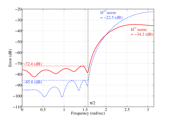
Figure 3. The gain of the error $E(z)=P(z)-Q(z)$ for $H^{\infty}$ optimization (solid) and finite-frequency min-max optimization (dash)

By the MATLAB codes given in the previous section, we design FIR filters for Problems 1 and 3. Let the FIR filter order $N=8$. The target filter is the second order lowpass Butterworth filter with cutoff frequency $\pi/2$. This can be computed by butter(2,1/2) in MATLAB. The weighting transfer function in Problem 1 is chosen by a 8th order lowpass Chebyshev filter, computed by cheby1(8,1/2,1/2) in MATLAB. The frequency band for Problem 3 is $\Omega=[0,\pi/2]$. Figure 3 shows the gain of the error $E(z):=P(z)-Q(z)$. We can see that the $H^{\infty}$ optimal filter (the solution of Problem 1), say $Q_{1}(z)$, shows the lower $H^{\infty}$ norm than the finite-frequency min-max design (the solution of Problem 3), say $Q_{2}(z)$. On the other hand, in the frequency band $[0,\pi/2]$, $Q_{1}(z)$ shows the larger error than $Q_{2}(z)$.

9. Conclusion

In this article, we consider four problems, FIR approximation and inverse FIR filtering of IIR filters by $H^{\infty}$ and finite-frequency min-max, which are fundamental in signal processing. By using KYP and generalized KYP lemmas, the problems are all solvable via semidefinite programming. We show MATLAB codes for the programming, and show examples of designing FIR filters.

References

- [1] B. A. Francis, A Course in Control Theory. Springer, 1987.
- [2] T. Iwasaki and S. Hara, “Generalized KYP lemma: unified frequency domain inequalities with design applications,” IEEE Trans. Autom. Control, vol. 50, pp. 41–59, 2005.
- [3] B. D. O. Anderson, “A system theory criterion for positive real matrices,” Siam Journal on Control and Optimization, vol. 5, pp. 171–182, 1967.
- [4] A. Rantzer, “On the Kalman–Yakubovich–Popov lemma,” Systems & Control Letters, vol. 28, no. 1, pp. 7–10, 1996.
- [5] J. Tuqan and P. P. Vaidyanathan, “The role of the discrete-time Kalman-Yakubovitch-Popov lemma in designing statistically optimum FIR orthonormal filter banks,” Proc. of ISCAS, vol. 5, pp. 122–125, 1998.
- [6] S. Boyd and L. Vandenberghe, Convex Optimization. Cambridge University Press, 2004.
- [7] W. J. Rugh, Linear Systems Theory. Prentice Hall, 1996.
- [8] M. Vidyasagar, “A state-space interpretation of simultaneous stabilization,” IEEE Trans. Autom. Control, vol. 33, no. 5, pp. 506–508, 1988.
- [9] A. V. Oppenheim and R. W. Schafer, Discrete-Time Signal Processing, 3rd ed. Prentice Hall, 2009.
- [10] Y. Yamamoto, B. D. O. Anderson, M. Nagahara, and Y. Koyanagi, “Optimizing FIR approximation for discrete-time IIR filters,” IEEE Signal Process. Lett., vol. 10, no. 9, 2003.
- [11] M. Nagahara and Y. Yamamoto, “ optimal approximation for causal spline interpolation,” Signal Processing, vol. 91, no. 2, pp. 176–184, 2011.
- [12] M. Nagahara and Y. Yamamoto, “Optimal noise shaping in modulators via generalized KYP lemma,” Proc. of IEEE ICASSP, vol. III, pp. 3381–3384, 2009.
-
[13]
Mathworks, Control System Toolbox Users Guide, 2010. [Online].
Available:
http://www.mathworks.com/products/control/ - [14] J. Löfberg, “Yalmip : A toolbox for modeling and optimization in MATLAB,” Proc. IEEE International Symposium on Computer Aided Control Systems Design, pp. 284–289, 2004. [Online]. Available: http://users.isy.liu.se/johanl/yalmip/
- [15] J. F. Sturm, Using SeDuMi 1.02, a MATLAB toolbox for optimization over symmetric cones, 2001. [Online]. Available: http://sedumi.ie.lehigh.edu/