Social distancing strategies against disease spreading
Abstract
The recurrent infectious diseases and their increasing impact on the society has promoted the study of strategies to slow down the epidemic spreading. In this review we outline the applications of percolation theory to describe strategies against epidemic spreading on complex networks. We give a general outlook of the relation between link percolation and the susceptible-infected-recovered model, and introduce the node void percolation process to describe the dilution of the network composed by healthy individual, , the network that sustain the functionality of a society. Then, we survey two strategies: the quenched disorder strategy where an heterogeneous distribution of contact intensities is induced in society, and the intermittent social distancing strategy where health individuals are persuaded to avoid contact with their neighbors for intermittent periods of time. Using percolation tools, we show that both strategies may halt the epidemic spreading. Finally, we discuss the role of the transmissibility, , the effective probability to transmit a disease, on the performance of the strategies to slow down the epidemic spreading.
keywords:
Epidemics, Percolation, Complex Networks1 Introduction
Increasing incidence of infectious diseases such as the SARS and the recent A(H1N1) pandemic influenza, has led to the scientific community to build models in order to understand the epidemic spreading and to develop efficient strategies to protect the society [1, 2, 3, 4]. Since one of the goals of the health authorities is to minimize the economic impact of the health policies, many theoretical studies are oriented to establish how the strategies maintain the functionality of a society at the least economic cost.
The simplest model that mimics diseases where individuals acquire permanent immunity, such as the influenza, is the pioneer susceptible-infected-recovered (SIR) model [5, 6, 7, 8]. In this epidemiological model the individuals can be in one of the three states: i) susceptible, which corresponds to a healthy individual who has no immunity, ii) infected, a non-healthy individual and iii) recovered, that corresponds to an individual who cannot propagate anymore the disease because he is immune or dead. In this model the infected individuals transmit the disease to the susceptible ones, and recover after a certain time since they were infected. The process stops when the disease reaches the steady state, , when all infected individuals recover. It is known that, in this process, the final fraction of recovered individuals is the order parameter of a second order phase transition. The phase transition is governed by a control parameter which is the effective probability of infection or transmissibility of the disease. Above a critical threshold , the disease becomes an epidemic, while for the disease reaches only a small fraction of the population (outbreaks) [8, 9, 10, 11]. The first SIR model, called random mixing model, assumes that all contacts are possible, thus the infection can spread through all of them. However, in realistic epidemic processes individuals have contact only with a limited set of neighbors. As a consequence, in the last two decades the study of epidemic spreading has incorporated a contact network framework, in which nodes are the individuals and the links represent the interactions between them. This approach has been very successful not only in an epidemiological context but also in economy, sociology and informatics [5]. It is well known that the topology of the network, the diverse patterns of connections between individuals plays an important role in many processes such as in epidemic spreading [12, 13, 14, 15]. In particular, the degree distribution that indicates the fraction of nodes with links (or degree ) is the most used characterization of the network topology. According to their degree distribution, networks are classified in i) homogeneous, where node’s connectivities are around the average degree and ii) heterogeneous, in which there are many nodes with small connectivities but also some nodes, called hubs or super-spreaders, with a huge amount of connections. The most popular homogeneous networks is the Erdös Rényi (ER) network [16] characterized by a Poisson degree distribution . On the other hand, very heterogeneous networks are represented by scale-free (SF) distributions with , with , where represents the heterogeneity of the network. Historically, processes on top of complex networks were focused on homogeneous networks since they are analytically tractable. However, different researches showed that real social [17, 18], technological [19, 20], biological [21, 22] networks, etc, are very heterogeneous.
Other works showed that the SIR model, at its steady state, is related to link percolation [7, 8, 23, 10]. In percolation processes [24], links are occupied with probability . Above a critical threshold , a giant component (GC) emerges, which size is of the order of the system size ; while below there are only finite clusters. The relative size of the GC, , is the order parameter of a geometric second order phase transition at the critical threshold . Using a generating function formalism [25, 26, 27], it was shown that the SIR model in its steady state and link percolation belong to the same universality class and that the order parameter of the SIR model can be exactly mapped with the order parameter of link percolation [8]. For homogeneous networks the exponents of the transitions have mean field (MF) value, although for very heterogeneous network the exponents depend on .
Almost all the researches on epidemics were concentrated in studying the behavior of the infected individuals. However, an important issue is how the susceptible network behaves when a disease spreads. Recently, Valdez et. al. [28, 29] studied the behavior of the giant susceptible component (GSC) that is the functional network, since the GSC is the one that supports the economy of a society. They found that the susceptible network also overcomes a second order phase transition where the dilution of the GSC during the first epidemic spreading can be described as a “node void percolation” process, which belongs to the same universality class that intentional attack process with MF exponents.
Understanding the behavior of the susceptible individuals allows to find strategies to slow down the epidemic spread, protecting the healthy network. Various strategies has been proposed to halt the epidemic spreading. For example, vaccination programs are very efficient in providing immunity to individuals, decreasing the final number of infected people [30, 31]. However, these strategies are usually very expensive and vaccines against new strains are not always available during the epidemic spreading. As a consequence, non-pharmaceutical interventions are needed to protect the society. One of the most effective and studied strategies to halt an epidemic is quarantine [32] but it has the disadvantage that full isolation has a negative impact on the economy of a region and is difficult to implement in a large population. Therefore, other measures, such as social distancing strategies can be implemented in order to reduce the average contact time between individuals. These “social distancing strategies” that reduce the average contact time, usually include closing schools, cough etiquette, travel restrictions, etc. These measures may not prevent a pandemic, but could delay its spread.
In this review, we revisit two social distancing strategies named, “social distancing induced by quenched disorder” [33] and “intermittent social distancing” (ISD) strategy [29], which model the behavior of individuals who preserve their contacts during the disease spreading. In the former, links are static but health authorities induce a disorder on the links by recommending people to decrease the duration of their contacts to control the epidemic spreading. In the latter, we consider intermittent connections where the susceptible individuals, using local information, break the links with their infected neighbors with probability during an interval after which they reestablish the connections with their previous contacts. We apply these strategies to the SIR model and found that both models still maps with link percolation and that they may halt the epidemic spreading. Finally, we show that the transmissibility does not govern the temporal evolution of the epidemic spreading, it still contains information about the velocity of the spreading.
2 The SIR model and Link Percolation
One of the most studied version of the SIR model is the time continuous Kermack-McKendrick [34] formulation, where an infected individual transmits the disease to a susceptible neighbor at a rate and recovers at a rate . While this SIR version has been widely studied in the epidemiology literature, it has the drawback to allow some individuals to recover almost instantly after being infected, which is a highly unrealistic situation since any disease has a characteristic recovering average time. In order to overcome this shortcoming, many studies use the discrete Reed-Frost model [35], where an infected individual transmits the disease to a susceptible neighbor with probability and recovers time units after he was infected. In this model, the transmissibility that represents the overall probability at which an individual infects one susceptible neighbor before recover, is given by
| (1) |
It is known that the order parameter , which is the final fraction of recovered individuals, overcomes a second order phase transition at a critical threshold , which depends on the network structure.
One of the most important features of the Reed-Frost model (that we will hereon call SIR model) is that it can be mapped into a link percolation process [7, 8, 36, 23], which means that is possible to study an epidemiological model using statistical physic tools. Heuristically, the relation between SIR and link percolation holds because the effective probability that a link is traversed by the disease, is equivalent in a link percolation process to the occupancy probability . As a consequence, both process have the same threshold and belong to the same universality class. Moreover, each realization of the SIR model corresponds to a single cluster of link percolation. This feature is particularly relevant for the mapping between the order parameters of link percolation and for epidemics, as we will explain below.
For the simulations, in the initial stage all the individuals are in the susceptible state. We choose a node at random from the network and infect it (patient zero). Then, the spreading process goes as follows: after all infected individuals try to infect their susceptible neighbor with a probability , and those individuals that has been infected for time steps recover, the time increases in one. The spreading process ends when the last infected individual recovers (steady state).
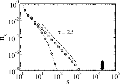
In a SIR realization, only one infected cluster emerges for any value of . In contrast, in a percolation process, for many clusters with a cluster size distribution are generated [37]. Therefore we must use a criteria to distinguish between epidemics (GC in percolation) and outbreaks (finite clusters). The cluster size distribution over many realizations of the SIR process, close but above criticality, has a gap between small clusters (outbreaks) and big clusters (epidemics). Thus, defining a cutoff in the cluster size as the minimum value before the gap interval, all the diseases below are considered as outbreaks and the rest as epidemics (see Fig. 1a). Note that will depend on . Then, averaging only those SIR realizations whose size exceeds the cutoff , we found that the fraction of recovered individuals maps exactly with (see Fig. 1b). For our simulations, we use for .
It can be shown that using the appropriate cutoff, close to criticality, all the exponents that characterizes the transition are the same for both processes [11, 38, 39]. Thus, above but close to criticality
| (2) | |||||
| (3) |
with [40]
| (6) |
The exponent of the finite cluster size distribution in percolation close to criticality is given by
| (9) |
For the SIR model and for a branching process (see Sec. 3), there is only one “epidemic” cluster, thus near criticality the probability of a cluster of size , , has exponent , where is given by Eq. (9) (see Fig. 1a). For SF networks with , in the thermodynamic limit, the critical threshold is zero, and there is not percolation phase transition. On the other hand, for and ER networks, all the exponents take the mean field (MF) values.
3 Mathematical approach to link percolation
Given a network with a degree distribution , the probability to reach a node with a degree by following a randomly chosen link on the graph, is equal to , where is the average degree. This is because the probability of reaching a given node by following a randomly chosen link is proportional to the number of links of that node and is needed for normalization. Note that, if we arrive to a node with degree following a random chosen link , the total number of outgoing links or branches of that node is . Therefore, the probability to arrive at a node with outgoing branches by following a randomly chosen link is also . This probability is called excess degree probability [41, 42].
In order to obtain the critical threshold of link percolation, let us consider a randomly chosen and occupied link. We want to compute the probability that through this link an infinite cluster cannot be reached. For simplicity, we assume to have a Cayley tree. Here we will denote a Cayley tree as a single tree with a given degree distribution. Notice that link percolation can be thought as many realizations of Cayley tree with occupancy probability , which give rise to many clusters. By simplicity we first consider a Cayley tree as a deterministic graph with a fixed number of links per node. Assuming that , the probability that starting from an occupied link we cannot reach the shell through a path composed by occupied links, is given by
| (10) |
Here, the exponent takes into account the number of outgoing links or branches, and is the probability that one outgoing link is not occupied plus the probability that the link is occupied (, at least one shell is reached) but it cannot lead to the following shell [5]. In the case of a Cayley tree with a degree distribution, we must incorporate the excess degree factor which accounts for the probability that the node under consideration has outgoing links and sum up over all possible values of . Therefore, the probability to not reach the generation can be obtained by applying a recursion relation
| (11) | |||||
| (12) |
where is the generating function of the excess degree distribution. As increases, and the probability that we cannot reach an infinite cluster is
| (13) |
Thus, the probability that the starting link connects to an infinite cluster is . From Eq (13), is given by
| (14) |
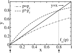
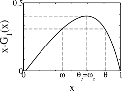
The solution of equation can be geometrically understood in Fig. 2 as the intersection of the identity line and , which has at least one solution at the origin, , for any value of . But if the derivative of the right hand side of Eq. (14) with respect to , , we will have another solution in . This solution has the physical meaning of being the probability that a randomly selected occupied link is connected to an infinite cluster. The criticality corresponds to the value of at which the curve has exactly slope equal one. Thus is given by [43]
| (15) |
For ER networks, we have . On the other hand, we can obtain the order parameter of link percolation , which represents the fraction of nodes that belongs to the giant cluster when a fraction of links are occupied in a random Cayley tree. The probability that a node with degree does not belong to the giant component is given by the probability that none of its links connect the node to the GC, , . Thus the fraction of nodes that belong to the GC is . Since the relative epidemic sizes in the SIR model maps exactly with the relative size of the giant component, we have that
| (16) |
where is the generating function of the degree distribution and is the non-trivial solution of Eq. (14) for . It is straightforward to show that for ER networks and thus . For pure SF networks, with , the generating function of the excess degree distribution is proportional to the poly-logarithm function , where is the Riemann function [42].
In the current literature, the epidemic spreading is usually described in terms of compartmental quantities, such as the fraction of infected or susceptible individuals during an epidemic, and very little has been done to describe how the disease affects the topology of the susceptible network that can be considered as the functional network. In the following section, we explain how an epidemic affects the structure of the functional network in the steady state.
4 Node Void Percolation and the SIR model
We define “active” links as those links pairing infected and susceptible individuals. During the epidemic spreading, the disease is transmitted across active links, leading in the steady state to a cluster composed by recovered individuals and clusters of susceptible individuals. Alternatively, the growing process of the infected cluster can also be described as a dilution process from the susceptible point of view. Under this approach, as the “infectious” cluster grows from a root, the sizes of the void clusters, those clusters composed by susceptible individuals, are reduced as in a node dilution process, since when a link is traversed a void cluster loses a node and all its edges. However, the susceptible nodes are not randomly uniform reached by the disease because they are chosen following a link. As a consequence higher degree nodes are more likely to be reached than the ones with small degrees. We will call “node void percolation” to this kind of percolation process in which the void nodes are not removed at random. In this dilution process, there exists a second critical value of the transmissibility (with ), above which the giant susceptible component (GSC) is destroyed.
Similarly to link percolation, in a Cayley tree (branching process) the analytical treatment for the dilution of the susceptible network uses a generating function formalism, that allows to compute the existence of a GSC and its critical threshold.
Considering the same growing infected cluster process as in the previous section, for large generations can also be interpreted as the probability that starting from a random chosen link, a path or branch leads to the GC. Thus, if we cannot reach a GC through a link, as we have a single tree, that link leads to a void node. Thus the probability to reach a void node through a link is given by
| (17) |
which is also the probability to reach a susceptible individual by following a link at a given transmissibility . It was shown that is a fundamental observable to describe the temporal evolution of an epidemic [28, 44, 45]. As in the usual percolation process, there is a critical threshold at which the susceptible network undergoes a second order phase transition. Above a GSC exists while at and below susceptible individuals belong only to finite components. As a consequence, the transmissibility needed to reach this point fulfills [29]
| (18) |
Therefore, from Eq (18) we obtain the self consistent equation
| (19) |
where is the solution of Eq. (19) and is given by [28] as can be seen in Appendix A and Ref. [28]. Thus for a virulent disease with , we have and therefore the size of the GSC [29]. The theoretical value of for a given value of can be obtained using an edge-based compartmental approach [44, 45, 28] that it is explained in Appendix A.
When , the size of the giant component and the distribution of void cluster’s sizes , behave with the distance to criticality as power laws.
| (20) | |||||
| (21) |
but in contrast to link percolation, their critical exponents have MF values, , and for homogeneous and heterogeneous networks [see Fig. 3 and Eqs. (6-9)]. Since two critical exponents are enough to characterize a phase transition, then all the critical exponents have MF values, as in an intentional attack percolation process independently of the network’s topology [46, 28].
These results are not only restricted to the steady state, but also can be extended to the temporal evolution of an epidemic spreading. It can be shown that during the spreading, the GSC dilutes as in a node void percolation process. In particular, for , there exists a critical time at which the GSC has the second order transition that we explained before. For further details, see Ref. [28]
All the concepts and tools previously introduced provide the basis for the study of the spread of an epidemic and the evolution of the GSC, that will be applied to the analysis of strategies against the epidemic spreading.
5 Social distancing induced by quenched disorder
Living in society implies that individuals are constantly interacting with each other. Interactions may take different forms, but those involving proximity or direct contact are of special interest because they are potential bridges to propagate infections. Empirical data suggest that human contacts follow a broad distribution [47, 48, 49]. These results support the idea that social interactions are heterogeneous, that means that individuals have a lot of acquaintances but just a few of them are close contacts. This heterogeneity between contacts can be thought as a network with quenched disorder on the links, wherein the disorder is given by a broad distribution. For example, if the weights represent the duration of the contacts between two individuals [42, 50, 51], the larger the weight, the easier is for an infection to traverse the link.
An important feature of the networks topology without disorder is the shortest average distance , defined as the minimum average number of connections between all pairs of nodes, which behaves as for ER networks [52] and as for very heterogeneous networks. This is why these networks are the called small or ultra small world [53]. It is known that the disorder can dramatically alter some topological properties of networks. Several studies have shown that when the disorder between connections is very broad or heterogeneous, also called strong disorder limit (SD), the network loses the small world property and the average distance goes as a power of for ER and SF networks with due to the fact that the SD can be related to percolation at criticality [54, 55, 56, 57]. However, the exact mapping between the order parameter of both second order phase transitions of percolation and SIR is not affected by a random disorder.
In the real life, the disorder in the network can be modified by health policies in order to, for example, delay the disease spreading allowing the health services to make earlier interventions [33]. Using different methods like broadcasting, brochures or masks distributions, the public health agencies can induce people to change their effective contact time and therefore the heterogeneity of the interactions. This strategy was tacitly used by some governments in the recent wave of influenza A(H1N1) epidemic in 2009 [4], but until now the effectiveness of the strategy and how it depends on the virulence and the structure of the disease has not been widely studied.
We study how the heterogeneity of the disorder affects the disease spreading in the SIR model for a theoretical quenched disorder distribution with a control parameter for its broadness. Using a theoretical disorder distribution given by,
| (22) |
where in [,1], and is the parameter which controls the width of the weight distribution and determines the strength of the disorder. Note that as increases, more values of the weight are allowed and thus the distribution is more heterogeneous.
In our weighted model the spreading dynamics follow the rules of the SIR model explained in Sec. 2, with a probability of infection that depends on the weight of each link, such that each contact in the network has infection probability , where represents the virulence characteristic of the disease in absence of disorder.
This type of weight has been widely used [55, 58, 57, 59] and it is a well known example of many distributions that allow to reach the strong disorder limit in order to obtain the mapping with percolation. With this weight distribution the transmissibility is given by Eq. (1) replacing by and integrating over the weight distribution [60], thus
| (23) | |||||
Note that, in the limit of we recover the classical SIR model (non disordered) with a fixed infection probability with . When there will be links in the network with zero weight and the strategy turns to a total quarantine with . For example, if , with , thus the transmissibility will be smaller than the intrinsic transmissibility of the disease without strategy for any , reducing the epidemic spreading.
In the following, we only consider those propagations that lead to epidemic states, and disregard the outbreaks. As the substrate for the disease spreading we use both, ER and SF networks. After the system reaches the steady state, we compute the mass of recovered individuals and the size of the functional network as a function of . Given an intrinsic transmissibility of the disease before the strategy is applied (see Eq. (1)), as increases, the impact of the disease on the population decreases as shown in Fig 4. We can see that in ER networks Fig 4(a) there is a threshold above which the epidemic can be stopped and only outbreaks occurs (epidemic free phase). However for very heterogeneous SF networks Fig 4(b), must increase noticeably in order to stop the epidemic spreading. For the steady magnitudes, the SIR process is always governed by the effective transmissibility given by Eq. (23), as shown in the inset of Fig. 4.
With the disorder strategy, the contact time between infected and susceptible individuals decreases hindering the disease spreading and protecting the functional network. We will refer to this defense mechanism of healthy individuals as “susceptible herd behavior”. As explained in Sec. 4, there is a that is the solution of Eq. (19) below which the susceptible herd behavior generates a GSC. In Fig. 5 we show the cluster size distribution of the susceptible individuals for and for for ER networks, which show that the exponent takes the mean field value of node percolation.
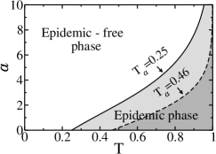
In Fig. 6 we plot the plane in order to show how depends on the intrinsic transmissibility of the disease and on the heterogeneity of the disorder . The full line in the plane corresponds to a , and separates the epidemic free phase (non colored region) from the epidemic phase (dark gray region). Note that is a parameter that could be controlled by the authorities, therefore the plane shows the required heterogeneity of the disorder needed to avoid an epidemic spreading depending on the virulence of the disease, characterized by the intrinsic . The dashed line corresponds to a , below which a GSC emerges. The light gray area indicates the phase where there is a coexistence of giant clusters of infected and susceptible individuals.
In this strategy, there are no restrictions on which individual to get away from. Another strategy could be to advise people to cut completely their connection with their infected contacts (when possible) for a given period of time. This kind of strategy will be analyzed in the next section.
6 Intermittent Social Distancing Strategy
In the previous strategy, individuals set a quenched disorder on the intensity of the interaction with their neighbors in order to protect themselves from the epidemic spreading. An alternative strategy consists of susceptible individuals that inactivate the interactions with their infected neighbors, but reestablish their contacts after some fixed time. This strategy that we call intermittent social distancing (ISD) strategy mimics a behavioral adaptation of the society to avoid contacts with infected individuals for a time interval, but without losing them permanently. This is an example of adaptive network where the topology coevolves with the dynamical process [61, 62].
Specifically, we study an intermittent social distancing strategy (ISD) in which susceptible individuals, in order to decrease the probability of infection, break (or inactivate) with probability their links with infected neighbors for intermittent periods of length .
We closely follow the presentation of this model from Ref. [29]. Assuming that the disease spreads with probability through the active links and that the infected individuals recovers after time steps, at each time step the infected individual tries first to transmit the disease to his susceptible neighbors, and then if he fails, susceptible individuals break their links with probability for a period .
These dynamic rules generate an intermittent connectivity between susceptible and infected individuals that may halt the disease spreading. In the limit case of , the ISD strategy is equivalent to a permanent disconnection, because when the link is restored the infected neighbor is recovered (or dead) and cannot transmit the disease anymore.
In order to compute the transmissibility for this strategy, we first introduce the case and then we generalize for any value of . For the case , let consider that an active link appears and denote the first time step of its existence as . At this time step, the active link tries to transmit the disease with probability , if it fails that link will be broken for the next time steps. After restoring that active link, the process is periodically repeated with period , until the disease is transmitted or the infected individual recovers. On the other hand, the time steps at which the link is active are located at times where is an integer number defined in the interval , where corresponds to the first time step, and is the maximum number of disconnection periods that leaves at the end at least one time step to transmit the disease. In particular, the probability to transmit the disease at the next time after disconnection periods is given by . Then summing over all possible values of , the total transmissibility [29] is given by
| (24) | |||||
For the case , first consider the example with only one disconnection period (), , and the infectious transmission at the time step , that is illustrated in the first line of Table 6. Note that in this case, there are only time units at which the link is active. Then, for this example the transmissibility is proportional to four factors: i) since there are active time steps at which the infected individual cannot transmit the disease, and at the last time unit the disease is transmitted, ii) , because the link is broken one time, iii) , because during active time steps the infected individual does not break the link except just before each inactive period and the last day, and iv) that is the total number of configurations in which we can arrange one inactive period in a period of length (this factor only takes into account the first time units, because the disease is transmitted at time . See the first line of Table 6).
Disconnected periods for a pair with (recovery
time), (disconnection period) and (time of
infection). The first column represents the number of disconnected
periods before , the second column is a typical
configuration, the third column is the probability of that
configuration and the fourth column is the number of ways to arrange
disconnected periods. In the second column, each cell correspond
to a time unit. The white cells represent the time units where a
link between the and the node exists, the gray ones
correspond to the disconnection period and in the black cells there
is no dynamic for the pair because the has been infected
and now the pair becomes . Notice that initially the link
cannot be broken because this disconnection only happens after that
the individual fails to infect the susceptible one, with
probability . Similarly, two disconnection periods must
be separated by at least one white cell.
u
Example
Probability
Binomial
Coefficient
![[Uncaptioned image]](/html/1308.2009/assets/x4.png)
![[Uncaptioned image]](/html/1308.2009/assets/x5.png)
In the general case, for all the values , the disease spreads with a total transmissibility given by,
| (25) |
In the first term of Eq. (25), is the probability that an active link is lost due to the infection of the susceptible individual at time step given that the active link has never been broken in the steps since it appears. In the second term of Eq. (25), denotes the probability that an active link is lost due to the infection of the susceptible individual at time given that the link was broken at least once in the first time units. The probability , which is only valid for is given by [29]
| (26) | |||||
where denotes the integer part function.
With the ISD strategy [29] the effective probability of infection between individual decreases, , and its minimal value corresponds to the extreme case of fully disconnection and . As a consequence if , the values of the parameters of our strategy can be tuned to stop the epidemic spreading.
In order to determine the effectiveness of the ISD strategy, we plot the epidemic size and the size of the functional susceptible network as a function of for ER and SF networks for different values of and . In Fig. 7, we can see that decreases as and increase compared to the static case . For the SF network the free-epidemic phase () is only reached for higher values of and than for ER networks. In any case, for both homogeneous and heterogeneous networks, the strategy is successful in protecting a giant susceptible component, for high values of and .
Similarly to the disorder strategy, in this model maps with a percolation process (see the insets of Fig. 7), and also when , the size distribution of the susceptible clusters behaves as (not shown here). In turn, in the ISD strategy the susceptible individuals change dynamically their connectivities with the infected neighbors, reducing the contact time between them. This generates an adaptive topology [61] in which the susceptible ones aggregate into clusters that produce a resistance to the disease. Therefore in the ISD strategy there is also a “susceptible herd behavior”.
In order to study the performance of the strategy protecting a GSC or preventing an epidemic phase, in Fig. 8 we plot the plane [where ] for different values of , using Eq. (25) for and .
In Fig 8 (a-b) starting from the case without strategy (line ) the epidemic phase and the phase without GSC shrink when and increase. Note that the light-gray area, delimited between the curves which corresponds to the extreme blocking periods and , displays the region of parameters controlled by the intervention strategy. In particular, given and , the maximum intrinsic transmissibility at which the strategy can prevent an epidemic phase or protect a GSC can be obtained using Eq. (24) for or respectively, and . On the other hand, note that in pure SF networks with and , , which implies that the strategy cannot halt the epidemic spreading for any value of the intrinsic transmissibility. However, is still finite on these topologies. Therefore, the ISD strategy can always protect the functional network for diseases with .
For the disorder strategy, we can reach similar conclusions because it is expected that the magnitudes in the steady state will behave in the same way for any strategy that is governed by the transmissibility. However, as we will show below, the evolution towards the steady state is different in both strategies.
7 Comparison between the ISD and the quenched disorder strategy
In Fig. 9 we plot the distribution of the duration time of an epidemic for the ISD strategy and the quenched disorder strategy for the same value of transmissibility .
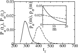
From the figure, we can see that the quenched disorder strategy generates larger duration times of the epidemic, , the disease spreading is slower than in the ISD strategy, which shows that the transmissibility does not govern magnitudes involved in the dynamical behavior. However, the discrepancy between the strategies can be explained from the transmissibility’s terms of Eqs. (23) and (25).
Lets denote the first time step of the existence of an active link as . Then using Eq. (23), the probability that the infected individual transmits the disease at time step , for the disorder quenched strategy, is given by
| (27) | |||||
Similarly, for the ISD strategy, the probability that the infected individual transmits at time is,
| (28) | |||||
From these probabilities, we compute the average time steps that takes to the disease to traverse an active link for several values of the parameters from both strategies, and we obtain that in the quenched disorder strategy the disease needs more time to infect a susceptible individual than in the ISD strategy (see the inset in Fig. 9). Thus it is expected that the final times in the former will be longer than in the latter. On the other hand, the ratio between the average times is compatible with ratio between the most probable final times of the distributions and . These results show that we can use minimal information, specifically the terms of the transmissibility in order to determine if the strategy slows down the epidemic spreading. Since one of the goals of the health authorities is to have more time to intervene, the average time could be used to compare, design or optimize mitigation strategies.
8 Summary
Percolation theory offers the possibility to explain the epidemic spreading and mitigation strategies in geometrical terms. In this brief review, we focused on the applications of percolation theory for the studying of social distancing strategies against the epidemic spreading of the SIR model.
We described the dilution of the network composed by susceptible individuals due to the disease spreading as a “node void percolation” process, and remark its importance in the development of strategies that aims to protect the functional network.
Using the SIR model for the disease propagation, we presented two social distancing strategies: the quenched disorder strategy and the intermittent social distancing strategy. We found that both strategies can control the effective transmissibility in order to protect the society. In particular, we described the protection of the GSC through the formation of a susceptible herd behavior. On the other hand, we showed that while the effective transmissibility control the final fraction of recovered individuals and the size of the GSC, it does not control observables that depends on the dynamical evolution of the process, such as the distribution of the duration of an epidemic.
One of the advantages of having two strategies that map with percolation theory is that we can fix the transmissibility in order to compare them and highlight the features of each strategy. Thus, for example, the knowledge of the mean time that a disease requires to traverse an active link, can be used to determine which strategy is better in delaying the epidemic spreading. Using the terms of the transmissibility, we showed that the quenched disorder strategy increases this average time, and thus the epidemic spreading is delayed compared to the ISD strategy. Our results show that a disorder strategy has a deeper effect on the spreading dynamics than a local adaptive topology.
Our findings could themselves have important applications for improving or designing mitigation strategies, since new strains of bacterias and viruses are continuously emerging or reemerging in multi-drug resistant forms, demanding the development of non-pharmaceutical intervention.
Acknowledgments
This work was financially supported by UNMdP and FONCyT (Pict 0293/2008). We thank C. E. La Rocca for useful comments and discussions.
Edge-Based Compartmental Model
The edge-based compartmental model [44, 45, 28], is a new theoretical framework to describe the dynamic of the disease spreading in the SIR model. Using this approach we can obtain the relation between and .
For clarity, we return to the SIR terminology, in which a void node corresponds to a susceptible individual and the node belonging to the giant percolating cluster (in a branching process) corresponds to a recovered individual.
In order to compute , we first calculate the fraction of susceptible individuals and then subtract the fraction of susceptible individuals belonging to finite size clusters.
Consider an epidemic disease in the steady state. We randomly choose a link and then give a direction to that link, in which the node in the target of the arrow is called the root, and the base is its neighbor. Denote as the probability that the neighbor has never transmitted the disease to the root, due to the fact that the neighbor is: (i) susceptible, or (ii) recovered, but he has never transmitted the disease to the root during its infectious period,
| (29) |
where . Therefore the probability that the root with connectivity is susceptible is , , an individual is susceptible only if none of his neighbors have transmitted the disease to him. Then, considering all the connectivities , the fraction of susceptible individuals in the steady state is . Note that can also be related to , since reaching a node through a link, it is susceptible only if none of its outgoing neighbors are connected to the giant recovered cluster, that is,
| (30) |
On the other hand, if we define as the probability that the neighbor is (i) susceptible but it does not belong to a GSC, or (ii) recovered, but he has never transmitted the disease to the root during its infectious period, then we have,
| (31) |
where is similar to , but restricted only to susceptible neighbors who belong to finite susceptible size clusters (see Eq. 30).
Then, from Eqs. (30) and (31) we obtain
| (32) |
Note that both hand sides of Eq. (32) has the form . In Fig. 10, we illustrate the solution of this equation.
Finally, for a given value of , we can solve Eqs. (30) and (32), in order to compute the relative size of the GSC, as
| (33) |
where is the fraction of void nodes belonging to finite void clusters (see Ref. [28] for details).
On the other hand, from Eq. (32) we can obtain the critical value at which vanishes, , when . Note that this happens only when , because is an strictly increasing function. In addition, since and fulfills Eq. (32), only at the maximum of (see Fig. 10). Then, denoting the maximum as , we have that
| (34) |
then,
| (35) |
Thus using Eq. (30), the critical threshold of the susceptible network is , which for ER networks .
Finally, we show the mean field exponent of as a function of .
Near the critical threshold of the susceptible network, the values of and from Eq. (32) are near to , in which we can approximate the function as a parabola. Thus , where and are constants. Doing some algebra on Eq. (32) around , we obtain
| (36) |
, is in the middle between and . Rewriting and as and , with , then near criticality, Eq. (33) can be approximated by
| (37) | |||||
On the other hand, near criticality we have that
| (38) | |||||
Therefore, using the relations (37) and (38), we obtain
| (39) |
with , that is a MF exponent. Note that we have not made any assumption on the form of or . Thus, this result is valid for homogeneous and heterogeneous networks.
References
- [1] P. Bajardi, C. Poletto, J. Ramasco, M. Tizzoni, V. Colizza and A. Vespignani, PLoS ONE 6, p. e16591 (2011).
- [2] V. Colizza, A. Barrat, M. Barthélemy and A. Vespignani, BMC Medicine 5, p. 34 (2007).
- [3] M. Lipsitch, T. Cohen, B. Cooper, J. M. Robins, S. Ma, L. James, G. Gopalakrishna, S. K. Chew, C. C. Tan, M. H. Samore, D. Fisman and M. Murray, Science 300, 1966 (2003).
- [4] D. Balcan, H. Hu, B. Goncalves, P. Bajardi, C. Poletto, J. J. Ramasco, D. Paolotti, N. Perra, M. Tizzoni, W. V. den Broeck, V. Colizza, and A. Vespignani, BMC Medicine 7, p. 45 (2009).
- [5] S. Boccaletti, V. Latora, Y. Moreno, M. Chavez and D. Hwang, Physics Reports 424, 175 (2006).
- [6] R. M. Anderson and R. M. May, Infectious Diseases of Humans: Dynamics and Control (Oxford University Press, Oxford, 1992).
- [7] P. Grassberger, Math. Biosci. 63, 157 (1983).
- [8] M. E. J. Newman, Physical Review E 66, p. 016128 (2002).
- [9] J. C. Miller, Phys. Rev. E 76, p. 010101 (2007).
- [10] E. Kenah and J. M. Robins, Phys. Rev. E 76, p. 036113 (2007).
- [11] C. Lagorio, M. V. Migueles, L. A. Braunstein, E. López and P. A. Macri, Physica A 388, 755 (2009).
- [12] E. M. Volz, J. C. Miller, A. Galvani and L. Ancel Meyers, PLoS Comput Biol 7, p. e1002042 (2011).
- [13] Marcel and J. J. H. Salathé, PLoS Comput Biol 6, p. e1000736(04 2010).
- [14] M. Boguñá, R. Pastor-Satorras and A. Vespignani, Epidemic spreading in complex networks with degree correlations, in Statistical Mechanics of Complex Networks, eds. R. Pastor-Satorras, M. Rubi and A. Diaz-Guilera, Lecture Notes in Physics, Vol. 625 (Springer Berlin Heidelberg, 2003) pp. 127–147.
- [15] L. D. Valdez, C. Buono, L. A. Braunstein and P. A. Macri, EPL 96, p. 38001 (2011).
- [16] P. Erdös and A. Rényi, On the evolution of random graphs. (Magyar Tud. Akad. Mat. Kut. Int. Közl., 1960).
- [17] M. E. J. Newman, Proc. Natl. Acad. Sci. USA 101, 5200 (2004).
- [18] A.-L. Barabási and R. Albert, Physica A 286, 509 (1999).
- [19] A.-L. Barabási, R. Albert and H. Jeong, Physica A 281, 69 (2000).
- [20] M. Faloutsos, P. Faloutsos and C. Faloutsos, Comput. Commun. Rev. 29, 251 (1999).
- [21] V. M. Eguíluz, D. R. Chialvo, G. A. Cecchi, M. Baliki and A. V. Apkarian, Phys. Rev. Lett. 94, p. 018102 (2005).
- [22] H. Jeong, S. P. Mason, A.-L. Barabasi and Z. N. Oltvai, Nature 411, p. 41 (2001).
- [23] L. A. Meyers, Bull. Amer. Math. Soc. 44, 63 (2007).
- [24] D. Stauffer and A. Aharony, Introduction to percolation theory (Taylor & Francis, 1985).
- [25] H. S. Wilf, Generatingfunctionology (A. K. Peters, Ltd., Natick, MA, USA, 2006).
- [26] D. S. Callaway, M. E. J. Newman, S. H. Strogatz and D. J. Watts, Phys. Rev. Lett. 85, 5468 (2000).
- [27] M. E. J. Newman, S. H. Strogatz and D. J. Watts, Phys. Rev. E 64, p. 026118 (2001).
- [28] L. D. Valdez, P. A. Macri and L. A. Braunstein, PLoS ONE 7, p. e44188 (2012).
- [29] L. D. Valdez, P. A. Macri and L. A. Braunstein, Phys. Rev. E 85, p. 036108 (2012).
- [30] M. J. Ferrari, S. Bansal, L. A. Meyers and O. N. Bjørnstad, Proceedings of the Royal Society B: Biological Sciences 273, 2743 (2006).
- [31] S. Bansal, P. Babak and M. L. Ancel, PLoS Med 3, p. e387 (2006).
- [32] C. Lagorio, M. Dickison, F. Vazquez, L. A. Braunstein, P. A. Macri, M. V. Migueles, S. Havlin and H. E. Stanley, Phys. Rev. E 83, p. 026102 (2011).
- [33] C. Buono, C. Lagorio, P. A. Macri and L. A. Braunstein, Physica A 391, 4181 (2012).
- [34] W. O. Kermack and A. G. McKendrick, Proc. Roy. Soc. Lond. A 115, 700 (1927).
- [35] N. T. J. Bailey, The Mathematical Theory of Infectious Diseases and Its Applications, 2nd ed. (Griffin, London, 1975).
- [36] J. C. Miller, Phys. Rev. E 80, p. 020901 (2009).
- [37] L. A. Meyers, B. Pourbohloul, M. Newman, D. M. Skowronski and R. C. Brunham, Journal of Theoretical Biology 232, 71 (2005).
- [38] Z. Wu, C. Lagorio, L. A. Braunstein, R. Cohen, S. Havlin and H. E. Stanley, Physical Review E 75, p. 066110 (2007).
- [39] S. Bornholdt and H. Schuster (eds.), Handbook of graphs and networks–From the Genome to the Internet (Wiley-VCH, Berlin, 2002).
- [40] R. Cohen, D. ben-Avraham and S. Havlin, Physical Review E 66, p. 036113 (2002).
- [41] M. E. J. Newman, SIAM Rev. 45, 167 (2003).
- [42] L. A. Braunstein, Z. Wu, Y. Chen, S. V. Buldyrev, T. Kalisky, S. Sreenivasan, R. Cohen, E. López, S. Havlin and H. E. Stanley, I. J. Bifurcation and Chaos 17, 2215 (2007).
- [43] R. Cohen, K. Erez, D. ben-Avraham and S. Havlin, Phys. Rev. Lett. 85, 4626 (2000).
- [44] J. C. Miller, A. C. Slim and E. M. Volz, Journal of The Royal Society Interface 9, 890 (2011).
- [45] J. C. Miller, Journal of Mathematical Biology 62, 349 (2011).
- [46] R. Cohen, K. Erez, D. ben-Avraham and S. Havlin, Phys. Rev. Lett. 86, 3682 (2001).
- [47] M. Karsai, M. Kivelä, R. K. Pan, K. Kaski, J. Kertész, A.-L. Barabási and J. Saramäki, Phys. Rev. E 83, p. 025102 (2011).
- [48] W. V. den Broeck, A. Barrat, V. Colizza, J.-F. Pinton, C. Cattuto and A. Vespignani, PLoS ONE 5, p. e11596 (2010).
- [49] J. Stehlé, A. Barrat, C. Cattuto, J.-F. Pinton, L. Isella and W. V. den Broeck, J. Theor. Biol. 271, 166 (2011).
- [50] T. Opsahl, V. Colizza, P. Panzarasa and J. Ramasco, Phys Rev Lett 101, p. 168702 (2008).
- [51] A. Barrat, M. Barthélemy, R. Pastor-Satorras and A. Vespignani, Proc. Natl. Acad. Sci. USA 101, p. 3747 (2004).
- [52] D. Watts and S. Strogatz, Nature 393, 440 (1998).
- [53] R. Cohen and S. Havlin, Phys. Rev. Lett. 90, p. 058701 (2003).
- [54] L. A. Braunstein, Z. Wu, Y. Chen, S. V. Buldyrev, T. Kalisky, S. Sreenivasan, R. Cohen, E. López, S. Havlin and H. E. Stanley, I. J. Bifurcation and Chaos 17, 2215 (2007).
- [55] L. A. Braunstein, S. V. Buldyrev, R. Cohen, S. Havlin and H. E. Stanley., Phys. Rev. Lett. 91, p. 168701 (2003).
- [56] S. Sreenivasan, T. Kalisky, L. A. Braunstein, S. V. Buldyrev, S. Havlin and H. E. Stanley., Phys. Rev. E 70, p. 046133 (2004).
- [57] M. Porto, S. Havlin, H. E. Roman and A. Bunde, Phys. Rev. E 58, p. 5205 (1998).
- [58] M. Cieplak, A. Maritan and J. R. Banavar, Phys. Rev. Lett. 76, p. 3754 (1996).
- [59] L. A. Braunstein, S. V. Buldyrev, S. Havlin and H. E. Stanley, Phys. Rev. E 65, p. 056128 (2001).
- [60] L. Sander, C. Warren, I. Sokolov, C. Simon and J. Koopman, Mathematical Biosciences 180, 293 (2002).
- [61] T. Gross and H. Sayama, Adaptive Networks: Theory, Models and Applications (Springer, 2009).
- [62] T. Gross, C. J. D. D’Lima and B. Blasius, Phys. Rev. Lett. 96, p. 208701 (2006).