Extended Techniques for Feedback Control of A Single Qubit

Abstract

The protection of quantum states is challenging for non-orthogonal states especially in the presence of noises. The recent research breakthrough shows that this difficulty can be overcome by feedback control with weak measurements. However, the state-protection schemes proposed recently work optimally only for special quantum states. In this paper, by applying different weak measurements, we extend the idea of the state-protection scheme to protect general states. We calculate numerically the optimal parameters and discuss the performance of the scheme. Comparison between this extended scheme and the earlier scheme is also presented.

In classical physics, it is possible in principle to acquire all information about the state of a classical system by precise measurements. Namely, the state of a single classical system can be precisely determined by measurements. This ensures the measurement-based classical feedback control and makes the feedback control beneficial to the manipulation of classical system.

For a quantum system, however, this is not possible: If the system is prepared in one of several non-orthogonal states, no measurement can determine determinately which state the system is really in. Furthermore, Heisenberg’s uncertainty principle imposes a fundamental limit on the amount of information obtained from a quantum system, and the act of measurement necessarily disturbs the quantum system 1 ; 2 ; 3 ; 4 ; 5 in an unpredictable way. This means when extend the measurement-based classical control theory to quantum system, we need careful examinations of the control scheme. The extension of the classical feedback to quantum systems can be used not only in quantum control 6 ; 7 ; 8 ; 9 ; 10 ; 11 , but also in quantum information processing, for example in the quantum key distribution 12 and quantum computing, as well as in other practical quantum technologies 13 .

Recent works in this field 14 ; 15 ; 16 suggested that we can balance the information gain from a measurement and the disturbance caused by the measurement via weak measurement. To be specific, in Ref.15 Branczyk et al. investigated the use of measurement and feedback control to protect the state of a qubit. The qubit is prepared in one of two non-orthogonal states in the $x-z$ plane of the Bloch sphere and subjected to noise. The authors shown that, in order to optimize the performance of the state protection, one must use non-projective measurements to balance the trade-off between information gain and disturbance. The measurement operators used in15 are among the $y-$ axis and the subsequent correction is a rotation about the $z-$axis. This scheme was realized recently 14 , where the stabilization of non-orthogonal states of a qubit against dephasing was experimentally reported. It is shown that the quantum measurements applied in the experiment play an important role in the feedback control. We should notice that the measurements used in14 are different to those in 15 , namely, its measurement operators are along the $z-$axis and the correction is about the $y-$ axis. Geometrically, for initial states in the $x-z$ plane, the dephasing noise can not map the initial states out of the $x-z$ plane, then all states including the initial states, the states passed the noise and measurements as well as the final stats are in the $x-z$ plane in14 , this is the difference between 14 and 15 from the geometric viewpoint. We will modify the measurement operators in 14 and use it in this paper.

With these knowledge in quantum information science 17 ; 18 ; 19 , one may wonder if the weak measurement used in the scheme is also the best one for the protection of general states? I.e., $M_{+}=\cos(\chi/2)|0\rangle\langle 0|+\sin(\chi/2)|1\rangle\langle 1|\,,$ and $M_{-}=\sin(\chi/2)|0\rangle\langle 0|+\cos(\chi/2)|1\rangle\langle 1|\,,$ are these measurements best for the protection of general states? Are there other measurements that can better the performance of the scheme for general states? In this paper, we shall shed light on this issue by introducing different measurements for the feedback control. We find that the scheme can be extended to protect general quantum states with the new weak measurement. We derive the performance and give the parameters best for the performance, a discussion on this extended scheme is also presented.

Consider two non-orthogonal states that we want to protect from noise,

$$|\psi_{\pm}\rangle{=}\cos\frac{\theta}{2}|+\rangle{\pm}e^{i\phi}\sin\frac{\theta}{2}|-\rangle,$$ (1)

with $|\pm\rangle{=}\frac{1}{\sqrt{2}}(|0\rangle\pm|1\rangle)$, the corresponding density matrices are given by $\rho_{\pm}{=}\mbox{$|\psi_{\pm}\rangle\langle\psi_{\pm}|$}$. Note that $|\psi_{+}\rangle$ and $|\psi_{-}\rangle$ are non-orthogonal and are more general than the states in 14 ; 15 , the overlapping of the two states is independent of $\phi$, but depends on $\theta$, $\langle\psi_{+}|\psi_{-}\rangle=\cos\theta.$ In fact, $|\psi_{\pm}\rangle$ are rotated about the $x$-axis with respect to the Branczyk’s one, this may offer a chance to improve the fidelity given by the previous proposals 14 ; 15 for general states of a qubit.

The qubit is subjected to dephasing noises 14 ; 15 . We shall use $\{|0\rangle,|1\rangle\}$ as the basis of the qubit Hilbert space, and define the Pauli operator $Z$ as $Z|0\rangle{=}|0\rangle,Z|1\rangle{=}{-}|1\rangle$, similar definitions are for Pauli matrices $X$ and $Y$. The dephasing noise can be described by a phase flip $Z$ with probability $p$ and with probability $1-p$ that the system remains unchanged. The density matrix of the qubit passed through the noisy channel is,

$$\rho^{{}^{\prime}}_{\pm}=(1-p)\rho_{\pm}+pZ\rho_{\pm}Z.$$ (2)

The purpose of this paper is to find better measurements and controls to send the qubit back as close as possible to its initial state. For this purpose, we use a quantum operation $\mathcal{C}$ as a map acting on the single qubit to describe the controls and measurements,

$$\mathcal{C}(\rho^{\prime})=Y_{+\eta}M^{\prime}_{+}\rho^{\prime}M_{+}^{\prime\dagger}Y_{+\eta}^{\dagger}+Y_{-\eta}M^{\prime}_{-}\rho^{\prime}M_{-}^{\prime\dagger}Y_{-\eta}^{\dagger}.$$

The notations of $Y$ and $M^{\prime}$ will be given later. To quantify the performance of $\mathcal{C}$, we use the average fidelity $\overline{F}$ 14 ; 15 between the noiseless input state and the corrected output state as a measure,

$$\overline{F} =\tfrac{1}{2}[\langle\psi_{+}|\mathcal{C}(\rho^{\prime}_{+})|\psi_{+}\rangle+\langle\psi_{-}|\mathcal{C}(\rho^{\prime}_{-})|\psi_{-}\rangle]$$

$$=\tfrac{1}{2}(F_{\psi_{+}}+F_{\psi_{-}})\,.$$ (3)

This measure quantifies the performance well when $|\psi_{+}\rangle$ and $|\psi_{-}\rangle$ are sent into the control with equal probability.

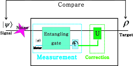
Figure 1: Illustration of the scheme. The meter qubit was entangled with the qubit (for protection) which has passed through the noise channel. After the measurement and correction, we can get a signal. Then we compare the signal with the initial state and apply a feedback control to the qubit. An average fidelity is define and used to determine the parameters in the feedback control. In the earlier scheme, the authors use a $|\varphi\rangle{=}\cos\frac{\chi}{2}|+\rangle{+}\sin\frac{\chi}{2}|-\rangle$ as the meter-qubit state, while in the present scheme a complex phase factor is introduced, i.e. the meter state is, $|\varphi\rangle{=}\cos\frac{\chi}{2}|+\rangle{+}e^{i\beta}\sin\frac{\chi}{2}|-\rangle.$

To find a good control procedure, we must first find the appropriate measurement which has to have the following two features. First, it must be a weak measurement, that is, it can not completely disturb the system. Second, it has to be strength-dependent, such that we can adjust the strength of the measurement as we need. This family of weak measurements in the logical basis $\{|0\rangle,|1\rangle\}$ can be written as,

$$M^{\prime}_{+} =\cos(\chi/2)|0\rangle\langle 0|+e^{i\beta}\sin(\chi/2)|1\rangle\langle 1|\,,$$ (4)

$$M^{\prime}_{-} =e^{i\beta}\sin(\chi/2)|0\rangle\langle 0|+\cos(\chi/2)|1\rangle\langle 1|\,.$$ (5)

In contrast to the measurements used in Ref.14 ; 15 ; 16 , $M_{+}=\cos(\chi/2)|0\rangle\langle 0|+\sin(\chi/2)|1\rangle\langle 1|\,,$ $M_{-}=\sin(\chi/2)|0\rangle\langle 0|+\cos(\chi/2)|1\rangle\langle 1|\,,$ a new parameter $\beta$ was introduced in this weak measurement 20 ; 21 . Here $\chi$ ranges from 0 to $\pi/2$ 20 , we can change the value of the parameter $\chi$ to adjust the strength of measurement. The corresponding positive measurement operators are given by $\Pi_{\pm}{=}M^{{}^{\prime}{\dagger}}_{\pm}M^{\prime}_{\pm}{=}[\mathbbm{1}\pm\cos{(\chi)}Z]/2$, with $\mathbbm{1}$ being the identity operator. Clearly, $\chi=0$ describes the projective measurement, while $\chi=\frac{\pi}{2}$, do nothing. At first glance, this proposal is trivial, i.e., the initial states (the state sent into protection) are rotated about $x-$axis in the Bloch sphere with respect to that in Ref.15 , by properly choosing $\beta$, the next measurements $M_{+}^{\prime}$ and $M_{-}^{\prime}$ may send them back, then the resulting states will return to that in the earlier proposal, and the performance can not be improved. We will show later that this is not the case.

Our main task is to figure out how the parameter $\beta$ affects the results of the control, and if the parameter $\beta$ can better the performance. The correction performed in this paper is the same as that in 14 , i.e., $Y_{\pm\eta}=\exp(\pm i\tfrac{1}{2}\eta Y)$ representing a rotation with an angle $\eta$ around the $y-$axis of the Bloch sphere. All parameters should be optimized for the performance of the control.

Straightforward calculation show that the average fidelity of the control is a function of $\theta,\phi,\eta,\chi,\beta$ and $p$,

$$\overline{F^{\prime}}(\theta,p,\chi,\eta,\phi,\beta)=\\ \tfrac{1}{2}\left[1+\cos\theta\cos\chi\sin\eta+\cos\eta\cos^{2}\phi\sin^{2}\theta\right.\\ +\tfrac{(1-2p)}{2}\sin\chi\left(2\cos\beta(\cos\eta\cos^{2}\theta+\sin^{2}\theta\sin^{2}\phi)\right.\\ \left.\left.-\sin\beta\sin\eta\sin^{2}\theta\sin 2\phi\right)\right]\,.$$ (6)

For each $\theta,$ $\phi$ and $p$, there are an optimum measurement strength $\chi,$ correction angle $\eta,$ and measurement parameter $\beta$, which maximizes the average fidelity. First we start with $\eta$. The $\eta$ which optimizes the average fidelity can be given by,

$$\eta_{\rm opt}(\theta,p,\chi,\phi,\beta)\\ =\arctan{\frac{\cos\theta\cos\chi-\tfrac{1}{2}(1-2p)\sin\beta\sin^{2}\theta\sin 2\phi\sin\chi}{\cos^{2}\phi\sin^{2}\theta+(1-2p)\cos^{2}\theta\sin\chi\cos\beta}}\,.\\$$ (7)

Substituting the optimum $\eta_{opt}$ into the average fidelity, we have,

$$\overline{F^{\prime}}(\theta,p,\chi,\phi,\beta)=\tfrac{1}{2}+\tfrac{1}{2}(1-2p)\cos\beta\sin^{2}\theta\sin^{2}\phi\sin\chi\\ +\frac{1}{2}\left[(\cos\theta\cos\chi-\tfrac{1}{2}(1-2p)\sin\beta\sin^{2}\theta\sin 2\phi\sin\chi)^{2}\right.\\ +(\cos^{2}\phi\sin^{2}\theta\left.+(1-2p)\cos^{2}\theta\sin\chi\cos\beta)^{2}\right]^{\tfrac{1}{2}}\,.$$ (8)

We can see that when $\phi=0$, $\overline{F^{\prime}}(\theta,p,\chi,\phi,\beta)$ reduces to

$$\overline{F^{\prime}}|_{\phi=0}=\frac{1}{2}+\frac{1}{2}\left[\cos^{2}\theta\sin^{2}\chi\right.$$ (9)

$$\left.+(\sin^{2}\theta+(1-2p)\cos^{2}\theta\sin\chi\cos\beta)^{2}\right]^{\frac{1}{2}}.$$

Obviously, $\beta=0$ maximize the average fidelity $\overline{F^{\prime}}$, this is exactly the case discussed in Ref. 14 ; 15 . So, for the initial states lying in the $xz-$ plane of the Bloch sphere, the weak measurements with $\beta=0$ already maximize the performance.

Figure 2: This figure shows how much our scheme improve the performance of the state protection for general qubit states. The improvement is quantified by $\delta_{F}$, which is plotted as a function of $\theta$ and $\phi$. For different $p$, the improvement is different, as (a), (b), (c) and (d) show. (a)$p=0.10;$ (b)$p=0.20;$ (c)$p=0.30;$ (d)$p=0.40.$

To find the optimal feedback control for $\phi\neq 0$, we follow the procedure in 14 . Here again $\theta$ and $\phi$ are related to the initial state of the qubit, while $p$ characterizes the noise and is regarded as a fixed value, $\chi$ and $\beta$ are related to the measurement procedure, $\eta$ denotes the correction parameter.

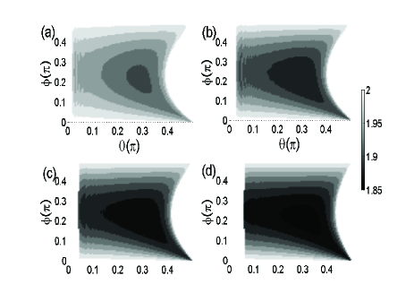
Figure 3: The $\beta$ which maximizes $\delta_{F}$ as a function of $\theta$ and $\phi$ for different $p$, (a)$p=0.10;$ (b)$p=0.20;$ (c)$p=0.30;$ (d)$p=0.40.$

By the same procedure as in the earlier works, we maximize the fidelity of the control over the remaining parameters $\chi$, $\theta,\phi,\beta$ and $p$. The analytical expression for the fidelity is complicated, so we choose to find the optimal parameters by numerical simulations. As aforementioned, we have already had the relations between the average fidelity and the initial parameters $\theta$ and $\phi$. We shall use $\delta_{F}{=}F^{\prime}_{opt}{-}F_{opt}$ to quantify the improved fidelity due to the parameter $\beta$, select results are presented in Fig.2, where $F^{\prime}_{opt}$ denotes the optimal fidelity in our paper, while $F_{opt}$ denotes that by the scheme in Ref.14 ; 15 , i.e., with $\beta=0.$ The optimized $\beta$ would depend on $\theta$ and $\phi$ and is shown in Fig.3.

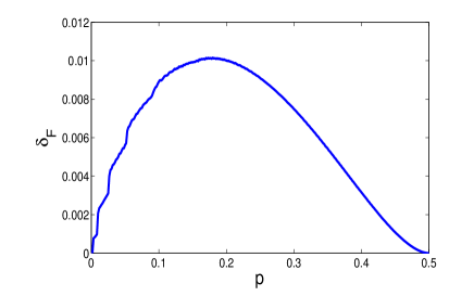
Figure 4: The fidelity difference $\delta_{F}$ versus $p$.

Fig.2 plots the improvement of the average fidelity as a function of the original states (characterized by $\theta$ and $\phi$) with different amount of noise (characterized by $p$). We note that there are no improvement for the following cases. If $p=0$, there is no noise and so the state is not perturbed, in this case the fidelity is 1 for all original states including $\phi=0$ and the measurement strength is $\chi=\frac{\pi}{2}$ (do nothing). When $\theta=\frac{\pi}{2}$, the state $|\psi_{+}\rangle$ and $|\psi_{-}\rangle$ are orthogonal, the earlier scheme gives unit fidelity, hence there is no room to improve the performance. When $\theta=0$ the two states are equal and point along the $x-$axis, these states are also the same as that in the earlier scheme, leading to zero improvement. If $\phi=\frac{\pi}{2}$, nothing should change since the two states would interchange by this control. Finally, when $\phi=0,$ the initial states return to the earlier scheme. Fig.3 shows the parameter $\beta$, which maximize the average fidelity as a function of the original states and the amount of noise $p$. As expected, non-zero maximal $\beta_{opt}$ exists. To show clearly the dependence of the improvement on the noise strength, we plot $\delta_{F}$ in Fig. 4 as a function of $p$. The maximal improvement arrived at about p=0.1800, the corresponding improvement is $\delta_{F}$=0.0102.

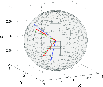
Figure 5: Bloch vectors of the original states(blue-solid), the resulting states by our scheme (red-dashed) and the resulting states in 15 (green-dotted). The parameters chosen are, $p=0.18,\eta=0.7913,\chi=0.8583,\beta=5.8905,\theta=1.0155,\phi=0.8976.$ All parameters except $p$ are in units of arc.

For developing an intuitive picture, we now take a snapshot for the states going through the control and measurement. Suppose the initial state is $|\psi_{+}\rangle$ with $\phi=\frac{\pi}{4}$, and let $\{|0\rangle,|1\rangle\}$ be a basis for the Hilbert space. In terms of density matrix, the initial state is

$$\rho_{+}=\frac{1}{2}\mathbbm{1}+\frac{1}{2}\cos\theta\cdot\sigma_{x}-\frac{\sqrt{2}}{4}\sin\theta\cdot\sigma_{y}+\frac{\sqrt{2}}{4}\sin\theta\cdot\sigma_{z},$$

This state lies in the $z=-y$ plane and points along the direction with an angle $\theta$ from the $x-$axis. The state passed the noisy channel is $\rho^{{}^{\prime}}_{+},$

$$\rho^{{}^{\prime}}_{+} = \frac{1}{2}\mathbbm{1}$$ (10)

$$+ (\frac{1}{2}-p)\cos\theta\cdot\sigma_{x}$$

$$+ \frac{\sqrt{2}}{2}(p-\frac{1}{2})\sin\theta\cdot\sigma_{y}$$

$$+ \frac{\sqrt{2}}{4}\sin\theta\cdot\sigma_{z},$$

we see that the $z-$component of the Bloch sphere remains unchanged, while the $x-$ and $y-$ components are shortened by $(1-2p)$ times due to the noise. The resulting state (unnormalized) immediately after the measurement is denoted by $\rho^{m}_{+},$ and it takes,

$$\rho^{m}_{+} = \frac{1}{2}(1+\frac{\sqrt{2}}{2}\cos\chi\sin\theta)\cdot\mathbbm{1}$$ (11)

$$+ \frac{1}{2}(1-2p)(\cos\beta\cos\theta+\frac{\sqrt{2}}{2}\sin\beta\sin\theta)\sin\chi\cdot\sigma_{x}$$

$$+ \frac{1}{2}(1-2p)(\cos\theta\sin\beta-\frac{\sqrt{2}}{2}\cos\beta\sin\theta)\sin\chi\cdot\sigma_{y}$$

$$+ \frac{1}{2}(\cos\chi+\frac{\sqrt{2}}{2}\sin\theta)\cdot\sigma_{z}.$$

Finally after the correction $Y_{+\eta}$, the unnormalized states has been mapped into,

$$\rho^{c}_{+} = \frac{1}{2}(1+\frac{\sqrt{2}}{2}\cos\chi\sin\theta)\cdot\mathbbm{1}$$ (12)

$$+ \frac{1}{2}\left(\sin\eta(\cos\chi+\frac{\sqrt{2}}{2}\sin\theta)+(1-2p)\cos\eta\sin\chi(\cos\beta\cos\theta+\frac{\sqrt{2}}{2}\sin\beta\sin\theta)\right)\cdot\sigma_{x}$$

$$+ \frac{1}{2}(1-2p)(\cos\theta\sin\beta-\frac{\sqrt{2}}{2}\cos\beta\sin\theta)\sin\chi\cdot\sigma_{y}$$

$$+ \frac{1}{2}\left(\cos\eta(\cos\chi+\frac{\sqrt{2}}{2}\sin\theta)+(-1+2p)\sin\eta\sin\chi(\cos\beta\cos\theta+\frac{\sqrt{2}}{2}\sin\beta\sin\theta)\right)\cdot\sigma_{z}.$$

Note that this state is also unnormalized. For a specific set of $\theta$, $\phi$ and $p$, the resulting state together with the resulting state in Ref.14 are illustrated in Fig. 5. This shows clearly that our resulting states are more close to the initial state than that given by the proposal with $\beta=0$. As shown, the new measurements can do better than the earlier one for general quantum states. This suggests that we can apply the new set of measurements to the feedback control. Now we examine how much this new scheme improves the fidelity with respect to the schemes with measurements ”do nothing” and ”strong measurement” (Helstrom).

Before processing, we briefly review the two special cases of the schemes, which differ from each other at the measurements: In the zero strength measurement, $\cos\chi=0$, namely, no measurement is applied. So the state protection with this measurement is called ”do nothing” (DN) control scheme; The projective measurement is applied with maximum strength ($\cos\chi=1$), with which the protection scheme had already been named as ”Helstrom” (H) scheme22 . In fact, DN control is actually not a measurement-based control because of no application of measurement to quantum states. And H scheme is not what we need, because it makes an unnecessary correction to the system. To quantify the fidelity difference between these schemes, we define

$$F_{imp}=F_{opt}^{\prime}-max\{F_{DN},F_{H}\}$$ (13)

as a measure to quantify the difference, where $F_{DN}$ is the fidelity of DN control scheme, while $F_{H}$ represents the fidelity of the H scheme.

Figure 6: $F_{imp}$ versus $\theta$ and $\phi$ with different $p$,(a)$p=0.10$; (b)$p=0.20$; (c)$p=0.30$; (d)$p=0.40.$ This figure shows the improvement of our scheme over the DN and H schemes.

We have performed numerical simulations for $F_{imp}$, selective results are presented in Fig.6 and Fig. 7. In Fig.6, we present $F_{imp}$ as a function of $\theta$ and $\phi$ for different $p$. A common feature is that $F_{imp}$ reach its maximum at around $\theta=\pi/4$ and $\phi=\pi/4$. For different $p$, the improvement in the fidelity is different.

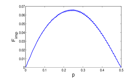
Figure 7: $F_{imp}$ as a function of $p$. In this figure, $F_{imp}$ is numerically optimized over $\theta$ and $\phi$ for each $p$. $p$ runs from 0 to 0.5, covering all possible choices.

To show the dependence of $F_{imp}$ on $p$ clearly, we plot the maximum $F_{imp}$ versus the parameter $p$ in Fig. 7 with different $\theta$ and $\phi$. As the figure shows, when $p=0.2501$, $F_{imp}$ reaches the maximum value 0.0662. Although the improvement is small, it can work under most conditions and it does improve the state protection over other schemes with different measurements16 . This tells that the scheme without the parameter $\beta$ is not the best scheme for state protection of general states.

It is illustrative to view the difference between our scheme (see Fig.8(Right top)) and the scheme (Fig.8(Left top)) in Ref.14 on the Bloch sphere. In Fig.8(Left top), we can see that the original states $|\psi_{+}\rangle$ and $|\psi_{-}\rangle$ (green) are shorten by the noise, but the $z-$component of the Bloch vector remains unchanged (pink vector on the Bloch sphere, i.e., $\rho^{\prime}_{\pm}$). The measurements lengthen the Bloch vectors(blue, i.e., $M_{+}^{\prime}\rho^{\prime}M_{+}^{\prime\dagger}$) and diminish the angle between the Bloch vector and the $z-$ axis. We should remind that the Bloch vectors remains in the $xz-$ plane in the whole process of measurements and controls, this is the core difference between the scheme in 14 and ours. This difference offers us a room to improve the performance of the control.

In our scheme, the original states are rotated about the $x-$axis with respect to the earlier scheme, see Fig.8(Right top). The effect of the noise is not only to shorten the length of the Bloch vector of the states, but also map the Bloch vector out of the plane of the original states. When the measurement is made, two things happen, as Fig.8 (Right top) shows. (1) The Bloch vector is lengthened, in other words, the state become more pure, see also Eq.(11). (2) The $x$ and $y$ components of the Bloch vector is mixed, in contrast to the proposal with $\beta=0$. As a consequence, the next rotation $Y_{\pm\eta}$ about the $y-$axis may make the resulting states (red vector) more close to the original states with respect to the earlier scheme.

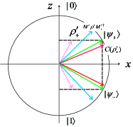
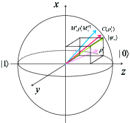
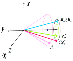
Figure 8: Bloch sphere representation of the initial states (green), the states after the noise (pink), the states after passing the measurement (blue) and correction (red). Left top is for the scheme in Ref.14 , while the Right top figure is for ours. Notice that the Left top figure shows only the $xz-$plane of the Bloch sphere, and the axis of the Bloch sphere in the Left and Right top figures are different. The Bloch vectors of the initial state, the state after the noise(post-noise state) and the state after the measurement(post-measurement state) form three cones, sharing an axis, i.e., the $y-$axis, which pass perpendicularly through the centre of the bases(see the bottom figure). The three cones have a common apes, i.e., the origin of the Bloch sphere. One optimal scheme is to use measurement operators that map the two post-noise states to the cone formed by the initial states as close as possible. The correction is a rotation about the $y-$axis, which would rotate the post-measurement states to the initial states as close as possible.

Both control schemes in 14 and 15 are optimal for depolarizing noise and states lying in the $x-z$ plane, the depolarizing noise keeps these particular states in the $x-z$ plane and maintains the trace distance between the two states. If the original states are not in the $x-z$ plane, the depolarizing noise can not maintain the trace distance between the two states and causes the plane in which the two states lie to rotate as the states pass through the depolarizing channel. The optimal control scheme will depend on the orientation of the post-noise states. From the optimality proof in Ref. 15 , we find that one optimal scheme is to use measurement operators to prolong the Bloch vectors of the post-noise states, and the correction is to bring the post-measurement states to the initial states as close as possible. The measurements and the correction are closely connected for a high performance. In the present scheme, the optimal scheme is to use measurement operators that can map the two post-noise states as close as possible to the cone formed by the initial states. Specifically, the Bloch vectors of the initial state, the post-noise state and the post-measurement state form three cones(see the bottom figure of Fig. 8), these cones share an axis: the $y-$axis, which pass perpendicularly through the centers of the bases. The three cones have a common apes, i.e., the origin of the Bloch sphere. One optimal scheme is to use measurement operators that map the two post-noise states very close to the initial-state-cone. The correction is a rotation about the $y-$axis, which would rotate the post-measurement states as close as possible to the initial states. This analysis simply consider the rotations of the axes of the Bloch sphere, to have a good performance, the length of the post-measurement state should be taken into account, this makes the optimization of $\beta$ complicated.

It is worth emphasizing that the angle rotated of our initial states is $\phi$. One may suspect that when the measurement cancels this rotation and send the states back to the $x-z$ plane, i.e., $\beta=\phi$, the optimal performance can be obtained. This intuition comes from the optimality proof in Ref.15 , however this is not true as we shall show below.

By using the average fidelity $\overline{F^{\prime}}(\theta,p,\chi,\eta,\phi,\beta)$ in Eq.(6), we can calculate $\frac{\partial\overline{F^{\prime}}}{\partial\beta}.$ From $\frac{\partial\overline{F^{\prime}}}{\partial\beta}|_{\beta=\beta_{c}}=0,$ $\beta_{c}$ follows, which maximize the average fidelity $\overline{F^{\prime}}$ and takes,

$$\tan\beta_{c}=-\frac{1}{2}\frac{\sin\eta\sin^{2}\theta\sin 2\phi}{\cos\eta\cos^{2}\theta+\sin^{2}\theta\sin^{2}\phi}.$$

Clearly, the $\beta$ that maximize the performance depends not only on $\phi$ and $\theta$, but also on $\eta$, namely, it connects closely with the correction $Y_{\pm\eta}$. When $\phi=0$, $\beta_{c}=0$, returning back to the earlier scheme. This observation can be understood as follows. We denote $U$ the rotation about the $x-$axis, which sends the initial state back to the $xz-$plane, i.e., $\rho_{\pm}=U\tilde{\rho}_{\pm}U^{\dagger}.$ Here, $\tilde{\rho}_{\pm}=\rho_{\pm}|_{\phi=0}$. Then the resulting state $\mathcal{C}(\rho^{\prime})$ can be written as,

$$\mathcal{C}(\rho^{\prime})=U\left(\tilde{Y}_{+\eta}\tilde{M}^{\prime}_{+}\tilde{\rho}^{\prime}\tilde{M}_{+}^{\prime\dagger}\tilde{Y}_{+\eta}^{\dagger}+\tilde{Y}_{-\eta}\tilde{M}^{\prime}_{-}\tilde{\rho}^{\prime}\tilde{M}_{-}^{\prime\dagger}\tilde{Y}_{-\eta}^{\dagger}\right)U^{\dagger},$$ (14)

where $\tilde{\rho}^{\prime}=(1-p)\tilde{\rho}+p\tilde{Z}\tilde{\rho}\tilde{Z},$ and $\tilde{(...)}=U^{\dagger}(...)U.$ This suggests that when the initial states are written as the same as that in the earlier scheme, the noise, measurement and the correction all need to change. Since $X$, $Y$ and $Z$ do not commute with each other, these changes are not trivial. We should emphasize that the effect of the noise given in Eq. (2) is to spoil the off-diagonal elements of the density matrix, or to shorten the $x-$ and $y-$component of the Bloch vector for any state, not only for the states lie in the $xz-$plane, so the aim of our scheme is to protect states against the same noise as that in the earlier scheme.

In conclusion, we introduce new measurements to better the state protection for a qubit. The average fidelity is calculated and discussed. Numerical optimizations over these parameters show that the new measurements can extend the state protection scheme from special states to general states. This scheme works for a wide range of initial states and generalize the scheme in the earlier works. The construction of the new proposal has several advantages. First, the initial states are more general, namely the corresponding Bloch vectors are allowed to lie outside the $xz-$plane, this extends the range of state protection and makes the scheme more realistic. The effect of the noise is to shorten the $x$ and $y$ components of the Bloch sphere, hence the noise is of dephasing. Second, we made use of a measurement which allow us to mix the $x-$ and $y-$components of the Bloch sphere, offering a room to improve the performance of the state protection. Finally, we note that the key elements to our scheme have already been experimentally demonstrated 14 , we expect that this extension of the earlier quantum control scheme is within reach of current technologies.   
  
This work is supported by the NSF of China under Grants Nos 61078011, 10935010 and 11175032.

References

- (1) A. C. Doherty, S. Habib, K. Jacobs, H. Mabuchi, and S. M. Tan, Phys. Rev. A 62, 012105 (2000).
- (2) A. C. Doherty, K. Jacobs, and G. Jungman, Phys. Rev. A 63, 062306 (2001).
- (3) H. M. Wiseman and A. C. Doherty, Phys. Rev. Lett. 94, 070405 (2005).
- (4) S. Mancini and H. M. Wiseman, Phys. Rev. A 75, 012330 (2007).
- (5) A. Shabani and K. Jacobs, Phys. Rev. Lett. 101, 230403 (2008).
- (6) M. A. Armen, J. K. Au, J. K. Stockton, A. C. Doherty, and H. Mabuchi, Phys. Rev. Lett. 89, 133602 (2002).
- (7) W. P. Smith, J. E. Reiner, L. A. Orozco, S. Kuhr, and H. M. Wiseman, Phys. Rev. Lett. 89, 133601 (2001).
- (8) J. Geremia, J. K. Stockton, and H. Mabuchi, Science 304, 270 (2004).
- (9) J. E. Reiner, W. P. Smith, L. A. Orozco, H. M. Wiseman, and J. Gambetta, Phys. Rev. A 70, 023819 (2004).
- (10) M. D. LaHaye, O. Buu, B. Camarota, and K. C. Schwab, Science 304, 74 (2004).
- (11) P. Bushev, D. Rotter, A. Wilson, F. Dubin, C. Becher, J. Eschner, R. Blatt, V. Steixner, P. Rabl, and P. Zoller, Phys. Rev. Lett. 96, 043003 (2006).
- (12) C. H. Bennett, Science 257, 752 (1992).
- (13) H. Rabitz, New J. Phys. 11, 105030 (2009).
- (14) G. G. Gillett, R. B. Dalton, B. P. Lanyon, M. P. Almeida, M. Barbieri, G. J. Pryde, J. L. Obrien, K. J. Resch, S. D. Bartlett, and A. G. White, Phys. Rev. Lett. 104, 080503 (2010).
- (15) A. M. Branczyk, P. E. M. F. Mendonca, A. Gilchrist, A. C. Doherty, and S. D. Bartlett, Phys. Rev. A 75, 012329 (2007).
- (16) X. Xiao and M. Feng, Phys. Rev. A 83, 054301 (2011).
- (17) D. P. DiVincenzo, Science 270, 255 (1995).
- (18) I. L. Chuang, R. Laflamme, P. W. Shor, and W. H. Zurek, Science 270, 1633 (1995).
- (19) A. Ekert and R. Josza, Rev. Mod. Phys. 68, 733 (1996).
- (20) M. A. Nielsen and I. L. Chuang, Quantum Computation and Quantum Information (Cambridge University Press, Cambridge, 2000).
- (21) N. Katz, M. Neeley, M. Ansmann, R. C. Bialczak, M. Hofheinz, E. Lucero, A. O Connell, H. Wang, A. N. Cleland, J. M. Martinis, and A. N. Korotkov , Phys. Rev. Lett. 101, 200401 (2008).
- (22) C. W. Helstrom, Quantum Detection and Estimation Theory, Mathematics in Science and Engineering Vol. 123 (Academic, New York, 1976).