Higher order extensions of the Gaussian effective potential

Abstract

A variational method is discussed, extending the Gaussian effective potential to higher orders. The single variational parameter is replaced by trial unknown two-point functions, with infinite variational parameters to be optimized by the solution of a set of integral equations. These stationary conditions are derived by the self-energy without having to write the effective potential, making use of a general relation between self-energy and functional derivatives of the potential. This connection is proven to any order and verified up to second order by an explicit calculation for the scalar theory. Among several variational strategies, the methods of minimal sensitivity and of minimal variance are discussed in some detail. For the scalar theory, at variance with other post-Gaussian approaches, the pole of the second-order propagator is shown to satisfy the simple first-order gap equation that seems to be more robust than expected. By the method of minimal variance, nontrivial results are found for gauge theories containing fermions, where the first-order Gaussian approximation is known to be useless.

I introduction

Variational methods are very useful in quantum mechanics, and quite often their use becomes mandatory when the interaction strength is too large. In quantum field theory, the use of variational methods has always been questioned because of the weight of high energy modes that prevents any reasonable physical result unless the trial functional has the exact high energy asymptotic behavior. Recently, a new interest has emerged on variational methodskogan ; reinhardt ; szcz because of the relevance of non-Abelian gauge theories that are known to be asymptotically free. The high energy asymptotic behavior of these theories is known exactly, while the low energy physics can only be accessed by numerical lattice simulations because of the large strength of the interaction that does not allow the use of standard perturbation theory. As a consequence, important problems like quark confinement and the low energy phase diagram of QCD still lack a consistent analytical description, and the development of nonperturbative variational techniques would be more than welcome in this important area of quantum field theory.

Another problem with variational methods is calculability: the energy is a functional of the quantum fields and, while in principle any trial functional could be chosen, the need of an analytically tractable theory makes the Gaussian functional the only viable choice. Thus, we are left with the Gaussian Effective Potential (GEP), which has been discussed by several authorsschiff ; rosen ; barnes ; stevenson and, at variance with perturbation theory, there is no obvious way to improve the approximation order by order.

Besides being a truly variational method, the GEP may also be regarded as a self-consistent theory since the proper self-energy vanishes at first order, and the Gaussian free-particle Green function is equal to the first-order function. The GEP has many merits and has been successfully applied to physical problems ranging from electroweak symmetry breakingibanez and scalar theoriesstevenson ; var ; light ; bubble in 3+1 spacetime dimensions, to superconductivity in bulk materialssuperc1 ; superc2 and filmskim , to non-Abelian gauge theoriessu2 and quite recently to the Higgs-top sector of the standard modelLR ; AF ; HT .

Even if the GEP usually gives a fairly good representation of reality, an extension of the Gaussian approximation has always been desirable. However, any attempt to improve the GEP has not been so successful, and most merits of the GEP seem to disappear at second order. For instance, the Post-Gaussian Effective Potential (PGEP) discussed by Stancu and Stevensonstancu is not a truly variational method (the exact effective potential cannot be shown to be smaller than the PGEP), it is not self-consistent, and it fails to reach a minimum for any finite value of the variational parameters (in most cases the vanishing of a second derivative is required).

In this paper, we point out that most of the shortcomings of the PGEP could be just a consequence of using a fixed shape for the two-point Gaussian correlator. We explore a more general extension of the GEP, where the best Gaussian two-point function is the solution of a nonlinear integral equation, a generalized stationary condition that replaces the simple first-order gap equation. At any order, the generalized stationary condition can be derived by the self-energy graphs, without having to write the effective potential. Order by order, that is possible because of the existence of a simple exact connection between the gap equation and the self-energy that allows for a direct derivation of the generalized gap equation by standard methods of perturbation theory. The connection between self-energy and gap equation generalizes the well-known property of self-consistency of the first-order GEP, which in turn is a consequence of the equivalence between the gap equation and the vanishing of the first-order self-energy.

For a scalar theory under general physical assumptions and for different choices of variational strategies, we show that the second-order two-point function is characterized by a self-consistent mass which is formally given by the same first-order Gaussian gap equation. Thus, the first-order gap equation seems to be more robust than expected.

The formalism can be extended to more general theories like gauge theories containing bosons and fermions and might be used for the development of variational approaches to strongly interacting sectors of the standard model. The simple case of a $U(1)$ gauge theory with a single fermion is discussed in some detail and, at variance with GEP and PGEP that are known to be useless for fermionsstancu ; stancu2 , the present method provides an integral equation with nontrivial solutions that can be evaluated by iterative numerical techniques.

In Section II, after a brief discussion on the viable variational strategies in field theory, an extension is presented where the finite set of variational parameters is replaced by a trial function that is equivalent to an infinite set of variational parameters. The method is illustrated by the simple model of a self-interacting scalar theory.

In Section III, the proof is given of a general connection between the functional derivative of the effective potential and the self-energy. The connection is shown to be valid order by order and plays a key role for determining the variational stationary conditions without having to write the effective potential. Up to second order the relation is verified in detail in the Appendix by a direct evaluation of the effective potential.

In Section IV, the second order extension of the GEP is described in some detail for the scalar theory. The methods of minimal sensitivity and of minimal variance are compared and shown to provide nonlinear integral equations. The analytical properties of the solution are studied and the pole of the second-order propagator is shown to satisfy the same first-order gap equation of the GEP.

In Section V, the method is extended to the simple $U(1)$ gauge theory with a single fermion, and the method of minimal variance is shown to be suited for a second-order variational approach to gauge theories. The stationary conditions provide a linear equation for the propagator with a nontrivial unique solution. A perturbative expansion of the result is shown to give back the standard equations of quantum electrodynamics.

In Section VI, the results of the paper are discussed with some concluding remarks.

Details on the derivation of the effective potential up to second order are reported in the Appendix.

II Generalizations of the Gaussian effective potential

The Post-Gaussian effective potential was discussed by Stancu and Stevensonstancu for the scalar theory with and without fermionsstancu2 . One of the main merits of the method is its use of the standard perturbative techniques for evaluating the effective potential while retaining a variational nature. In fact the method consists in a perturbative expansion around a trial zeroth-order two-point function that is then optimized by the variation of a parameter. Since the original Lagrangian does not depend on the variational parameter, the principle of minimal sensitivityminimal is enforced by requiring that the nth-order effective potential should be stationary with respect to the variation of the parameter. The resulting expansion turns out to be convergent even when the original interaction did not contain any small parameter. In the original PGEP the two-point function was taken as a free propagator with the mass that played the role of the variational parameter.

The method can be generalized as follows: the zeroth-order two-point function could be taken as a free unknown trial function, that is equivalent to deal with an infinite set of variational parameters. The variational constraint becomes an integral equation for the unknown trial two-point function, and the eventual solution would improve over the PGEP. We have infinitely more variational parameters while retaining the Gaussian shape of the functional that allows for calculability. Of course, no general proof can be given of the existence of a solution, and the problem has to be studied case by case. Moreover, several different variational constraints and strategies can be proposed in order to extend the method order by order, and the existence of a solution depends on the chosen strategy.

II.1 Variational methods and strategies

Consider a quantum field theory with action $S[\phi]$ depending on a set of quantum fields $\phi\equiv\{\phi_{n}\}$, and introduce shifted fields $h_{n}=\phi_{n}-\varphi_{n}$ where $\varphi$ is a set of constant backgrounds. We can always split the action as

$$S[\phi]=S_{0}[h]+S_{I}[h]$$ (1)

where the interaction term is defined as

$$S_{I}[h]=S[\varphi+h]-S_{0}[h]$$ (2)

and $S_{0}[h]$ is a trial functional that can be freely chosen. We take the $S_{0}$ quadratic in the fields $h$ in order to get Gaussian integrals that can be evaluated exactly. This functional can be thought to be the free action of a field theory, and we denote by $H_{0}$ the Hamiltonian of that theory, while $H$ is the Hamiltonian of the full interacting theory described by the action $S$. The effective action $\Gamma[\varphi]$ can be evaluated by perturbation theory order by order as a sum of Feynman diagrams according to the general path integral representation

$$e^{i\Gamma[\varphi]}=\int_{1PI}{\cal D}_{h}e^{iS[\varphi+h]}=\int_{1PI}{\cal D}_{h}e^{iS_{0}[h]}e^{iS_{I}[h]}$$ (3)

that is equivalent to the sum of all the one-particle-irreducible (1PI) vacuum diagrams for the action functional $S[\varphi+h]$, where $\varphi$ acts like a sourceweinbergII , and $S_{I}$ plays the role of the interaction. In general, the action terms $S_{0}$ and $S_{I}$ have an implicit dependence on $\varphi$ that is omitted for brevity. Denoting by $\langle X\rangle$ the quantum average

$$\langle X\rangle=\frac{\int_{1PI}{\cal D}_{h}e^{iS_{0}[h]}X}{\int{\cal D}_{h}e^{iS_{0}[h]}}$$ (4)

the effective action can be written as

$$i\Gamma[\varphi]=i\Gamma_{0}[\varphi]+\log\langle e^{iS_{I}}\rangle$$ (5)

where the zeroth-order contribution can be exactly evaluated since $S_{0}$ is quadratic

$$i\Gamma_{0}[\varphi]=\log\int{\cal D}_{h}e^{iS_{0}[h]}$$ (6)

and the remaining terms can be written by expansion of the logarithm in moments of $S_{I}$,

$$\log\langle e^{iS_{I}}\rangle=\sum_{n=1}^{\infty}i\Gamma_{n}[\varphi] =\langle iS_{I}\rangle+\frac{1}{2!}\langle[iS_{I}-\langle iS_{I}\rangle]^{2}\rangle$$

$$+\frac{1}{3!}\langle[iS_{I}-\langle iS_{I}\rangle]^{3}\rangle+\dots$$ (7)

which is equivalent to taking the sum of all connected 1PI vacuum diagrams arising from the interaction $S_{I}$, as emerges from a direct evaluation of the averages by Wick’s theorem. In this paper, we use the convention that $\Gamma_{n}$, $V_{n}$, $\Sigma_{n}$ represent the single nth-order contribution, while the sum of terms up to nth order are written as $\Gamma^{(n)}$, $V^{(n)}$, $\Sigma^{(n)}$, so that

$$i\Gamma^{(N)}=\sum_{n=0}^{N}i\Gamma_{n}.$$ (8)

The effective potential follows as $V(\varphi)=-\Gamma[\varphi]/\Omega$ where $\Omega$ is a total spacetime volume.

On the other hand, the effective potential is known to be the vacuum energy density $E$, and can be expanded around the ground state $|0\rangle$ of $H_{0}$ in powers of the interaction $H-H_{0}$,

$$E=E_{0}+E_{1}+E_{2}+\dots$$ (9)

where $E_{0}$ is the exact ground-state energy of $H_{0}$,

$$E_{0}=\langle 0|H_{0}|0\rangle$$ (10)

and $E_{1}$ is the first-order correction

$$E_{1}=\langle 0|H-H_{0}|0\rangle.$$ (11)

By a direct comparison of the expansions we see that $V_{n}=E_{n}$, and the sum of the first two terms must give the first-order approximation for the effective potential

$$V^{(1)}=E_{0}+E_{1}=\langle 0|H|0\rangle$$ (12)

which is the expectation value of the full Hamiltonian $H$ in the trial state $|0\rangle$. Any variation of the parameters in $S_{0}$ is equivalent to a variation of $H_{0}$ and its ground state $|0\rangle$. Thus, a stationary condition imposed on the first-order effective potential is equivalent to the standard variational method of quantum mechanics. The resulting optimized first-order effective potential is the Gaussian effective potential.

Extensions of the GEP are not trivial: the second-order approximation for the effective potential gives

$$V^{(2)}=\langle 0|H|0\rangle+E_{2}$$ (13)

and a variation of the free parameters in $S_{0}$ is not equivalent to a variation of the expectation value of $H$. Moreover, it is well known that the second-order correction $E_{2}$ is negative for any quantum mechanical system, and $V^{(2)}$ can be lower than the exact vacuum energy. Thus the simple search for a minimum of $V^{(2)}$ would not work. Since the exact action $S$ does not depend on the free parameters in $S_{0}$, any extension of the GEP requires a new prescription for determining the free parameters. There are at least three methods that have been suggested: a fixed variational basistedesco , the minimal sensitivityminimal , and the minimal variancesigma ; sigma2 .

(i) The parameters in $S_{0}$ might be fixed by the minimal of the first-order effective potential, that is a genuine variational method. Then the higher order contributions could be evaluated by perturbation theory with the parameters kept fixed, even if that would spoil the convergence of the expansion. The ground state $|0\rangle$ and the other eigenstates of $H_{0}$ are then used as a fixed basis set optimized by the first-order variational method, as shown in Ref.tedesco .

(ii) Since the exact effective potential does not depend on the variational parameters in $S_{0}$, the minimal sensitivity of $V^{(n)}$ as been proposed as a variational criterionminimal . At each order the parameters are fixed by the stationary point of the total effective potential (or its derivative when no solution occurs). The stationary condition changes order by order, and the parameters must be determined again at any order. This procedure has been proven to improve the convergence of the expansionminimal .

(iii) More recentlysigma ; sigma2 the search for the minimal variance has been shown to be a valuable variational criterion for determining the unknown parameters. It is based on the physical idea that in the exact eigenstates of an operator ${\cal O}$, the variance must be zero because $\langle{\cal O}{\cal O}\rangle=\langle{\cal O}\rangle^{2}$. For any Hermitian operator like $H$, the variance is a positive quantity, bounded from below, and the variational parameters can be tuned by requiring that the variance is minimal.

In quantum mechanics, the last method is not very useful because the accuracy of the standard variational approximation can be easily improved by a better trial wave function with more parameters. In field theory, calculability does not leave too much freedom in the choice of the wave functional that must be Gaussian. When the simple stationary condition fails, a second-order extension can be achieved by the method of minimal variance, as discussed in Ref.sigma . Actually, we can write the second-order contribution to the effective potential in Eq.(7) as

$$V_{2}=E_{2}=-\frac{\sigma_{I}^{2}}{2\Omega}$$ (14)

where $\sigma_{I}$ is the variance of the Euclidean action $S_{I}^{E}$,

$$\sigma_{I}^{2}=\langle(S^{E}_{I})\rangle^{2}-\langle(S^{E}_{I})^{2}\rangle.$$ (15)

That follows immediately from Eq.(7) by Wick rotating as the operator $(iS)$ becomes the Euclidean action $(iS)\to-S^{E}$, while the quantum action $i\Gamma\to-V/\Omega$. Eq.(14) is in agreement with the general requirement that $E_{2}<0$. The variance would be zero if $|0\rangle$ were an exact eigenstate of $S_{I}$, while a minimal variance is expected to optimize the convergence of the expansion. The free parameters can be fixed by a stationary condition for the second-order term of the effective potential $V_{2}$. Then the optimized variational basis can be used for the evaluation of the higher order correction, as for the method of Ref.tedesco . At variance with that method, the second-order correction is used instead of the first-order one, and that would be useful whenever the simple first-order method should fail, as in gauge theories.

II.2 Generalization to infinite parameters

The higher order extensions of the GEP can be generalized to the case of infinite variational parameters. The method is illustrated in this section by the simple model of a self-interacting scalar theory. The Lagrangian reads

$${\cal L}=\frac{1}{2}\partial^{\mu}\phi\>\partial_{\mu}\phi-\frac{1}{2}m_{B}^{2}\phi^{2}-\lambda\phi^{4}$$ (16)

In the spirit of background field method let us introduce a shifted field $h=\phi-\varphi$ where $\varphi$ is a constant background. The action functional $S[\phi]$ can be written as

$$S[\varphi+h]= \frac{1}{2}\int h(x)g_{B}^{-1}(x,y)h(y){\rm d}^{4}x{\rm d}^{4}y$$

$$+\int\left(\frac{1}{2}m_{B}^{2}h^{2}-V_{c}[\varphi+h]\right){\rm d}^{4}x$$ (17)

where $V_{c}$ is the classical potential

$$V_{c}[\phi]=\frac{1}{2}m_{B}^{2}\phi^{2}+\lambda\phi^{4}$$ (18)

while $g_{B}^{-1}(x,y)$ is the bare inverse propagator

$$g_{B}^{-1}(x,y)=(-\partial_{\mu}\partial^{\mu}-m_{B}^{2})\delta^{4}(x-y).$$ (19)

Let us denote by $g(x,y)$ a trial unknown two-point function, and write the action functional as

$$S[\varphi+h]=S_{0}[h]+S_{I}[h]$$ (20)

where $S_{0}$ plays the role of the zeroth-order action functional

$$S_{0}[h]=\frac{1}{2}\int h(x)g^{-1}(x,y)h(y){\rm d}^{4}x{\rm d}^{4}y$$ (21)

and $S_{I}$ is the interaction term

$$S_{I}[h] =\frac{1}{2}\int h(x)\left[g_{B}^{-1}(x,y)-g^{-1}(x,y)\right]h(y){\rm d}^{4}x{\rm d}^{4}y$$

$$+\int\left(\frac{1}{2}m_{B}^{2}h^{2}-V_{c}[\varphi+h]\right){\rm d}^{4}x.$$ (22)

An implicit dependence on $\varphi$ is assumed in $g$, $S_{0}$, and $S_{I}$. Of course, the trial function $g^{-1}$ cancels in the total action $S[\varphi+h]$, which is exact and cannot depend on it. Thus, this formal decomposition holds for any arbitrary choice of the trial function, provided that the integrals converge.

The effective action $\Gamma[\varphi]$ can be evaluated by perturbation theory order by order as a sum of Feynman diagrams according to the general path integral representation of Eq.(3) that is equivalent to the sum of all 1PI vacuum diagrams for the action functional $S[\varphi+h]$, where $\varphi$ acts like a source. According to our decomposition of the action functional, we must associate the trial propagator $g(x,y)$ to the free-particle lines of the diagrams, while the vertices are read from the interaction terms in $S_{I}$. The effective action follows order by order as the sum of connected diagrams according to Eqs.(6) and (7). The zeroth-order contribution follows from Eq.(6),

$$V_{0}(\varphi)=-\frac{i}{2}\int\frac{{\rm d}^{4}k}{(2\pi)^{4}}\log\left[\frac{i}{2\pi}g^{-1}(k)\right]$$ (23)

where a Fourier transform $g^{-1}(k)$ has been introduced for the trial function $g^{-1}(x,y)\equiv g^{-1}(x-y)$, while according to Eq.(19) the bare propagator reads $g_{B}^{-1}(k)=k^{2}-m_{B}^{2}$.

Higher order terms follow by Eq.(7) and can be described by standard Feynman diagrams in terms of connected 1PI graphs. The vertices are extracted from the interaction Eq.(22) that yields the interaction Lagrangian

$${\cal L}_{int}=v_{0}+v_{1}h(x) +v_{3}h^{3}(x)+v_{4}h^{4}(x)$$

$$+\int h(x)v_{2}(x,y)h(y){\rm d}^{4}y$$ (24)

where

$$v_{0} =-V_{c}(\varphi)$$

$$v_{1} =-\varphi m_{B}^{2}-4\lambda\varphi^{3}$$

$$v_{2} =\frac{1}{2}(g_{M}^{-1}-g^{-1})$$

$$v_{3} =-4\lambda\varphi$$

$$v_{4} =-\lambda$$ (25)

and the modified bare propagator $g_{M}^{-1}(k)=k^{2}-M^{2}$ is defined in terms of the shifted mass

$$M^{2}=m_{B}^{2}+12\lambda\varphi^{2}.$$ (26)

Up to second order, the connected 1PI vacuum diagrams are shown in Fig.1 with their symmetry factors. The first-order contribution is given by the sum of the tree, one-loop, and two-loop graphs in the first row of Fig.1,

$$i\Gamma_{1}[\varphi] =i\Omega v_{0}+\int iv_{2}(x,y)ig(y,x){\rm d}^{4}x{\rm d}^{4}y$$

$$+3iv_{4}\int ig(x,x)ig(x,x){\rm d}^{4}x.$$ (27)

Figure 1: Connected vacuum 1PI graphs for the Lagrangian Eq.(24), up to second order. The trial propagator $g$ is reported as a straight line, while the vertices are defined in Eq.(25). The symmetry factors are displayed below the graphs.

Neglecting a constant term and dividing by a spacetime volume $\Omega$, the first-order contribution to the effective potential reads

$$V_{1}(\varphi) =V_{c}(\varphi)-\frac{i}{2}\int\frac{{\rm d}^{4}k}{(2\pi)^{4}}g^{-1}_{M}(k)g(k)$$

$$+3\lambda\left[\int\frac{{\rm d}^{4}k}{(2\pi)^{4}}ig(k)\right]^{2}$$ (28)

Adding the zeroth-order term of Eq.(23), the first-order effective potential can be written as

$$V^{(1)}(\varphi)=V_{c}(\varphi)+I_{1}[g]+3\lambda(I_{0}[g])^{2}-\frac{i}{2}\int\frac{{\rm d}^{4}k}{(2\pi)^{4}}g^{-1}_{M}(k)g(k)$$ (29)

where the functionals $I_{n}[g]$ have been defined as a generalization of the GEP and PGEP notation of Ref.stancu :

$$I_{0}[g] =\int\frac{{\rm d}^{4}k}{(2\pi)^{4}}ig(k)$$

$$I_{1}[g] =-\frac{i}{2}\int\frac{{\rm d}^{4}k}{(2\pi)^{4}}\log\left[\frac{i}{2\pi}g^{-1}(k)\right]$$

$$I^{(n)}[g] =n!i\int[ig(x,y)]^{n}{\rm d}^{4}x\>{\rm d}^{4}y.$$ (30)

All the divergent integrals are supposed to be regularized by a cutoff or other regularization scheme.

While the technique is based on perturbation theory, the approximation is valid even when there are no small parameters, provided that the effective potential is optimized by a variational criterion. In fact the interaction is defined in terms of the unknown trial function $g$, and its variation has an effect on both $S_{0}$ and $S_{I}$. The optimal choice of this pair should be the one that makes the effects of the interaction $S_{I}$ smaller in the vacuum of $S_{0}$. A stationary condition can be imposed by requiring that the functional derivative is zero. For instance, the principle of minimal sensitivity would require that, at a given order, the trial function $g$ satisfies the stationary condition

$$\frac{\delta V^{(n)}}{\delta g}=0.$$ (31)

In general this is a nonlinear integral equation for the unknown function $g$. Unfortunately we have no general proof of the existence of a solution, and the problem should be studied order by order.

At first order we require that

$$0=\frac{\delta V^{(1)}}{\delta g(k)}=\frac{i}{2}\left(g^{-1}(k)-g_{M}^{-1}(k)+12\lambda I_{0}[g]\right)$$ (32)

and find the simple solution

$$g^{-1}(k)=k^{2}-M_{1}^{2}$$ (33)

where the mass $M_{1}$ is the solution of the first-order gap equation

$$M_{1}^{2}=m_{B}^{2}+12\lambda\varphi^{2}+12\lambda I_{0}[g]$$ (34)

By inserting the self-consistent solution of Eqs.(34) and (33) in Eq.(29), we obtain the standard GEPstevenson ; stancu . Thus, at first order, the present method is equivalent to the GEP. The extra freedom on the shape of $g$ does not add anything to the first-order approximation, and the best $g$ maintains the form of a free-particle propagator. On the other hand, the shape of the optimized propagator tells us that the wave function renormalization is negligible in the self-interacting scalar theory, as confirmed by several lattice calculations. Moreover we can show that the first-order proper self-energy vanishes, so that the first-order propagator is equal to the optimized function $g$ that can be regarded as a self-consistent solution at first order. The graphs contributing to the self-energy are reported in Fig.2 up to second order (tadpole graphs are not included). The proper first-order term is the sum of the tree and the one-loop graphs in the first row,

Figure 2: Self-energy graphs for the Lagrangian Eq.(24), up to second order. The trial propagator $g$ is reported as a straight line, while the vertices are defined in Eq.(25). The symmetry factors are displayed below the graphs. We recognize two first-order graphs in the first row, four 1PI graphs in the second row (proper self-energy), and four reducible graphs in the last row. Tadpole graphs are not included.

$$-i\Sigma_{1}=i(g^{-1}_{M}-g^{-1})+12iv_{4}\int\frac{{\rm d}^{4}k}{(2\pi)^{4}}ig(k)$$ (35)

yielding

$$\Sigma_{1}(k)=g^{-1}(k)-k^{2}+m_{B}^{2}+12\lambda\varphi^{2}+12\lambda I_{0}[g]$$ (36)

which vanishes if the function $g$ in Eq.(33) satisfies the first-order gap equation Eq.(34). Actually, by inspection of Eq.(32), we can see that

$$\frac{\delta V^{(1)}}{\delta g(k)}=\frac{i}{2}\Sigma_{1}.$$ (37)

This consistency relation is a special case of a more general relation between self-energy and functional derivatives of the effective potential. In the next sections we will generalize the result to any order and to theories containing fermions.

For a second-order extension of the method, the trial function $g$ could be determined by the method of minimal sensitivity as the solution of the stationary condition

$$\frac{\delta V^{(2)}}{\delta g}=\frac{\delta}{\delta g}(V_{0}+V_{1}+V_{2})=0$$ (38)

or by the method of minimal variance as the solution of the stationary condition

$$\frac{\delta V_{2}}{\delta g}=0$$ (39)

These are integral equations for the unknown function $g$, and their solution is equivalent to the optimization of infinite parameters. In both cases, we would need the functional derivative of the second-order term $V_{2}$. However, by a generalization of Eq.(37), the higher order stationary conditions can be derived through a simpler path that makes use of the self-energy, without having to write the effective potential.

III Connection to self-energy

It is useful to develop a general method for the direct evaluation of the functional derivatives that appear in most of the variational approaches. We give proof of a general relation between self-energy and functional derivatives of the effective potential. For the sake of simplicity, we discuss the case of the self-interacting scalar theory, while the extension to more complex theories containing Bose and Fermi fields is quite straightforward. An extension to fermions is discussed below in Section V.

At each order, we find that

$$\frac{\delta V_{n}}{\delta g(k)}=\frac{i}{2}\left(\Sigma_{n}(k)-\Sigma_{n-1}(k)\right)$$ (40)

where $V_{n}$ and $\Sigma_{n}$ are the nth-order contribution to the effective potential and to the self-energy respectively, and no tadpole graph has been included in the self-energy (as is usually the case at the minimum of $V$ where $\delta V/\delta\varphi=0$ and the tadpoles cancel exactly). The relation can be taken to be valid even for $n=1,0$, provided that we define $\Sigma_{-1}=0$ and $i\Sigma_{0}=2\delta V_{0}/\delta g$. As a corollary, we find that the total nth-order effective potential $V^{(n)}$ satisfies

$$\frac{\delta V^{(n)}}{\delta g(k)}=\frac{i}{2}\Sigma_{n}(k)$$ (41)

and the vanishing of the functional derivative is equivalent to the vanishing of the nth-order contribution to the self-energy. In the special case of $n=1$, we recover Eq.(37) which is equivalent to the vanishing of the total self-energy and to the self-consistency of the optimized $g$ for the GEP, as discussed at the end of the previous section.

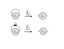
Figure 3: Correspondence between vacuum and self-energy graphs: in the upper row, vacuum 1PI connected graphs of order $n$ give connected self-energy graphs of order $n$ (without tadpoles) when operating with a partial functional derivative $\delta/\delta g$ according to Eq.(42); in the lower row, vacuum 1PI connected graphs of order $n$ give connected self-energy graphs of order $n-1$ (without tadpoles) when operating with a functional derivative of the vertex $v_{2}$.

The proof follows by Wick’s theorem and inspection of the diagrams. First of all, let us recall a general relation between the vacuum diagrams without any external line and the self-energy two-point diagrams with two external vertices where two external lines can be attached. All diagrams contributing to the nth order self-energy can be drawn by taking n interaction terms, picking up a pair of fields, and contracting all other fields according to Wick’s theorem. There is a contribution for each chosen pair of external fields. If we contract the external fields, we close the two-point diagram by a line and obtain a vacuum nth-order diagram without external lines and vertices, as shown in Fig.3. All vacuum diagrams can be drawn by picking up a pair of fields in all the possible ways, writing all the corresponding two-point diagrams, and then closing them by a line. As a consequence of Wick’s theorem, this procedure ensures that we find the correct symmetry factors. The argument can be reversed, and provided that we inserted the correct symmetry factors, if we cut a line in any possible way in all the nth-order vacuum diagrams, we obtain all the nth-order two-point diagrams contributing to the self-energy. Actually, an overall 2 factor must be added because of the permutation of the external fields in the two-point function. Using Feynman rules in momentum space, for any internal particle line, a factor $ig(k)$ is included and integrated over $k$. The functional derivative $\delta/\delta(ig)$ deletes a factor $ig$ and its corresponding integration; thus, it is equivalent to the cut of an internal line in all the possible ways, with the correct factor coming out from the derivative. Thus, denoting by $-i\Omega{\cal V}_{n}$ and $-i\Sigma_{n}$ the sum of all the nth-order vacuum and two-point graphs, respectively,

$$\left(\frac{\delta{\cal V}_{n}}{\delta g(k)}\right)_{\displaystyle{v_{2}}}=\frac{i}{2}\Sigma_{n}(k).$$ (42)

Here by $\delta/\delta g$ we mean the explicit partial derivative with the vertex $v_{2}$ kept fixed, while a total functional derivative would operate on the vertex $v_{2}$ also. In vacuum diagrams, the nonlocal two-point vertex $v_{2}$ is only present inside loops that have the following general form:

$$\int\frac{{\rm d}^{4}k}{(2\pi)^{4}}\dots ig(k)\cdot iv_{2}(k)\cdot ig(k)\dots$$ (43)

and by insertion of the vertex definition Eq.(25), we see that for each of them the total functional derivative acquires the extra term

$$\frac{\delta}{\delta g(p)}\left[\frac{{\rm d}^{4}k}{(2\pi)^{4}}\dots ig(k)\cdot iv_{2}(k)\cdot ig(k)\dots\right]=$$

$$=\left[\dots ig(p)i\frac{\partial v_{2}(p)}{\partial g(p)}ig(p)\dots\right]=\left[\dots\left(-\frac{i}{2}\right)\dots\right]$$ (44)

where the functional derivative only acts on the vertex. The effect of the derivative is the opening of the loop where the vertex was, yielding a two-point graph with a vertex less, as shown in Fig.3. At a given order, all the $v_{2}$ insertions in vacuum diagrams are in one-to-one correspondence with all the possible pairs of external fields that can be picked up for drawing two-point diagrams. Again, provided that the correct symmetry factors were included, Wick’s theorem ensures that the functional derivative of all $v_{2}$ insertions in ${\cal V}_{n}$ yields the sum of all two-point diagrams of order $n-1$, with the correct factor that comes out from the derivative. Thus, inserting the factor $-i/2$ coming out from the derivative of the vertex in Eq.(44), and adding the result of the partial derivative Eq.(42), the total functional derivative is

$$\frac{\delta{\cal V}_{n}}{\delta g(k)}=\frac{i}{2}\left[\Sigma_{n}(k)-\Sigma_{n-1}(k)\right].$$ (45)

Of course, here ${\cal V}_{n}$ and $\Sigma_{n}$ contain all kinds of terms including disconnected diagrams and tadpoles.

It is not difficult to understand that in Eq.(45), disconnected diagrams for $\Sigma_{n}$ are in correspondence with disconnected or reducible diagrams for ${\cal V}_{n}$, while self-energy diagrams containing tadpoles can only generate reducible vacuum diagrams. On the other hand, connected self-energy diagrams without tadpoles always generate 1PI connected vacuum diagrams when the two-point graph is closed with a line or a $v_{2}$ vertex, and 1PI connected vacuum diagrams always generate connected self-energy diagrams without tadpoles when a line or a $v_{2}$ vertex is cut by the functional derivative. When restricting to 1PI connected vacuum diagrams, ${\cal V}_{n}$ becomes the nth-order contribution to the effective potential $V_{n}$, and then Eq.(40) holds, provided that $\Sigma_{n}$ contains all connected self-energy graphs without tadpoles.

IV Second-order extensions of GEP

The first-order stationary condition Eq.(32) has been shown to be equivalent to the gap equation of the GEP Eq.(34) yielding the simple free-particle propagator of Eq.(33). As discussed in Section II, the second-order extension of the GEP is not trivial. Here, we study in more detail the second-order stationary conditions that emerge by the methods of minimal sensitivity Eq.(38) and minimal variance Eq.(39), for the self-interacting scalar theory. The stationary conditions are derived by the self-energy according to Eq.(40).

IV.1 Stationary conditions

By the method of minimal sensitivity, the generalized second-order stationary condition Eq.(38) reads

$$\frac{\delta V^{(2)}}{\delta g(k)}=\frac{i}{2}\Sigma_{2}(k)=0$$ (46)

where Eq.(41) has been used with $n=2$. Thus, the second-order gap equation is equivalent to the vanishing of the second-order contribution to the self-energy, ignoring tadpoles. All the second-order self-energy graphs are displayed in Fig.2. Adding together the four 1PI graphs in the second line, the proper second-order self-energy can be written as

$$\Sigma^{\star}_{2}(k)=-12v_{4}I_{\Sigma 1}+v_{3}^{2}J_{3}(k)+v^{2}_{4}J_{4}(k).$$ (47)

where $I_{\Sigma 1}$, $J_{3}(k)$, and $J_{4}(k)$ are new functionals of $g$. The functional $I_{\Sigma 1}$ does not depend on $k$ and is defined as

$$I_{\Sigma 1}=\int\frac{{\rm d}^{4}k}{(2\pi)^{4}}i[g(k)]^{2}\Sigma_{1}(k).$$ (48)

It generalizes the functional $I_{0}$ by the inclusion of a self-energy insertion in the loop, and arises from the sum of the first pair of second-order graphs in Fig.2. The functionals $J_{n}(k)$ carry an explicit dependence on $k$ and are defined as

$$J_{n}(k) =n\cdot n!\int g(k+\sum_{j=1}^{n-2}k_{j})\prod_{j=1}^{n-2}\left[ig(k_{j}){\frac{{\rm d}^{4}k_{j}}{(2\pi)^{4}}}\right]=$$

$$=\frac{i\delta I^{(n)}}{\delta g(k)}$$ (49)

where the last equality follows by evaluating the integrals $I^{(n)}$ in Eq.(30) in momentum space. Here the functionals $J_{3}$ and $J_{4}$ arise from the third and fourth 1PI graphs respectively, as displayed in Fig.2. The four reducible second-order graphs can be easily expressed in terms of $\Sigma_{1}$ yielding for the total second-order self-energy

$$\Sigma_{2}(k)=\Sigma_{2}^{\star}(k)+g(k)[\Sigma_{1}(k)]^{2}.$$ (50)

The condition of minimal sensitivity Eq.(46) then reads

$$\Sigma_{2}^{\star}(k)=-g(k)[\Sigma_{1}(k)]^{2}.$$ (51)

The derivation of this second-order stationary condition was made quite simple by the use of self-energy graphs and their connection to the functional derivatives of the effective potential. However the same equation could be derived by the more cumbersome calculation of the vacuum diagrams in Fig.1, followed by the functional derivative of all terms. Since it is instructive to examine the connection between the two methods, in the Appendix the effective potential is evaluated up to second order and its functional derivative is compared with the self-energy, term by term, showing a perfect agreement with Eq.(46).

By the method of minimal variance, the generalized second-order stationary condition Eq.(39) reads

$$\frac{\delta V_{2}}{\delta g(k)}=\frac{i}{2}(\Sigma_{2}(k)-\Sigma_{1}(k))=0$$ (52)

where Eq.(40) has been used with $n=2$. That is equivalent to imposing $\Sigma_{2}=\Sigma_{1}$. In terms of proper self-energies the condition of minimal variance can be written as

$$\Sigma_{2}^{\star}(k)=-g(k)[\Sigma_{1}(k)][\Sigma_{1}(k)-g^{-1}(k)]$$ (53)

and differs from the condition of minimal sensitivity Eq.(51) for the term $g^{-1}$ in the last factor.

Despite the simple shape of the resulting stationary conditions Eqs.(51),(53), these are nonlinear integral equations for $g$, and we cannot even prove the existence of a solution. It would be interesting to look for a numerical solution, but that is out of the aim of the present paper.

In the PGEP of Ref.stancu the trial function $g$ is forced to be the same as for the first-order approximation, but with a mass $M_{2}$ that should satisfy a second-order gap equation coming out from the condition of minimal sensitivity. Actually, they find no solution for their single variational parameter $M_{2}$ (their second-order effective potential is never stationary). That does not mean that the integral equation Eq.(51) has no solution, since the trial function $g$ has infinite degrees of freedom in our generalized approach. On the other hand, with the same constraint of a free-particle $g$, with a single variational mass parameter, the method of minimal variance has been shown to give a solutionsigma . In fact the variance is bounded, and it is more likely to have a minimum compared to $V^{(2)}$ that could even be unbounded according to Eq.(13). On the same footing, that does not mean that the integral equation (53) must have a solution, but it is a good physical argument for its existence.

IV.2 Analytical properties of solutions

Even without having derived the effective potential, some interesting consequences of the stationary equations can be studied. In fact, the present method allows for a study of the existence and properties of the solution without having to write down the effective potential.

Let us suppose that a function $g$ does exist, satisfying one of the stationary conditions Eqs.(51) or (53), and let us look at the analytical properties of this function. We can prove that the single-particle pole of the function $g$ must be at $k=M_{1}$, where $M_{1}$ is the solution of the first-order gap equation (34). That does not mean that the pole does not change, because the function $g$ in Eq.(34) must be the solution of the second-order stationary equation instead of the simple first-order solution Eq.(33). In other words, the second-order extension does not change the Gaussian gap equation but changes the shape of the function $g$ from its first-order free-particle form. That would also explain why no solution is found for the stationary condition in the PGEP of Ref.stancu where a free-particle trial function is used. The lack of any solution could be the sign of having chosen a wrong trial function. On the other hand, the first-order gap equation (34) seems to be more robust than expected by the PGEP analysis.

The proof of the above statement comes from a more careful inspection of Eqs.(51) and (53). Let us suppose that a solution $g(k)$ does exist, and that its single-particle pole is at $k=m$. In other words we are assuming that $k=m$ is the first singular point on the real axis, while other singularities or cuts may occur for $k>m$. We are going to prove that $m=M_{1}$, as defined in Eq.(34).

If Eqs.(51) or (53) hold, and $g$ has a pole in $k=m$, then the proper self-energy $\Sigma_{2}^{\star}(k)$ must have a pole unless $\Sigma_{1}$ vanishes. In this special point $k=m$, the two stationary conditions Eqs.(51) and (53) are equivalent because $g^{-1}(m)=0$. In $\Sigma^{\star}_{2}(k)$, the dependence on $k$ comes from the functionals $J_{3}(k)$ and $J_{4}(k)$. These are functionals of $g$ and cannot have a pole for $k<2m$ and $k<3m$, respectively. That is obvious in Euclidean space where the pole $g$ becomes imaginary and gives the long-range behavior of the Fourier transform $g(x)\sim exp(-mx)$. The functional $J_{n+1}(k)$ is the Fourier transform of $[g(x)]^{n}\sim exp(-n\cdot mx)$ and cannot have a pole for $k<n\cdot m$. That is a well-known property of graphs with multiparticle intermediate states like the one-loop and two-loop sunrise graphs that give the $J_{3}$ and $J_{4}$ terms. Then the function $\Sigma_{1}(k)$ must have a first-order zero in $k=m$ at least, supposing it to be a generally analytical function of $k$. As a by-product, $\Sigma^{\star}_{2}$ must have a zero in $k=m$ as well, in order to satisfy Eqs.(51) or (53). Then, inserting $\Sigma_{1}(m)=0$ and $g^{-1}(m)=0$ in Eq.(36), we obtain

$$m^{2}=m_{B}^{2}+12\lambda\varphi^{2}+12\lambda I_{0}[g]$$ (54)

which means that $m$ satisfies the first-order gap equation, i.e. $m=M_{1}$.

Denoting by $G_{(n)}$ the nth-order propagator, as obtained by standard perturbation theory with the interaction ${\cal L}_{int}$ of Eq.(24), we saw that $G_{(1)}=g$ at first order, i.e. the first-order approximation is self-consistent since $\Sigma_{1}$ vanishes identically. Setting $\varphi$ at its physical value, at the minimum of the effective potential where $\delta V/\delta\varphi=0$, all tadpole graphs cancel exactly in the self-energy, and the second-order propagator can be written in terms of proper self-energy insertions as

$$G_{(2)}^{-1}=g^{-1}-\Sigma_{1}-\Sigma_{2}^{\star}$$ (55)

and inserting Eq.(36) we obtain

$$G_{(2)}^{-1}(k)=k^{2}-M_{1}^{2}-\Sigma_{2}^{\star}(k)$$ (56)

which still has a pole in $k=M_{1}$ since $\Sigma_{2}^{\star}(M_{1})=0$. Thus, the pole is still self-consistent even if $g$ is not, since $g(k)\not=G_{(2)}(k)$ in the second-order approximation, and a non-vanishing wave function renormalization can be extracted by the residue of the pole.

While the present results are suggestive, they are all based on the hypothesis that without other constraints, at least one of the stationary conditions Eqs.(51) or (53) might have a solution. Moreover, we have not addressed the issue of renormalization: most of the integrals are divergent and, while a simple cut-off regularization would be enough in the case of an effective theory, renormalization of the bare parameters would be an interesting aspect to be studied. Again, perturbative techniques can be used as shown in Ref.stancu , even if the result has a genuine variational nature.

V Gauge interacting Fermions

For fermions, variational methods like GEP and PGEP are known to be uselessstancu2 , as the methods just reproduce the known results of perturbation theory. Thus, gauge theories with interacting fermions seem to be an interesting test for the generalized higher order extension of the GEP. The failure of the first-order GEP is a simple consequence of the minimal interaction that in gauge theories does not admit any first-order vacuum graph. It is mandatory to use higher order approximations, and the method of minimal variance seems to be suited to the case.

Quantum electrodynamics (QED) is the simplest $U(1)$ theory of interacting fermions. Let us consider the basic theory of a single massive fermion interacting through an Abelian gauge field

$${\cal L}=\bar{\Psi}(i\mathrlap{\!\not{\phantom{\partial}}}\partial+e{\mathrlap{\>\not{\phantom{A}}}A}-m)\Psi-\frac{1}{4}F^{\mu\nu}F_{\mu\nu}-\frac{1}{2}(\partial_{\mu}A^{\mu})^{2}$$ (57)

where the last term is the gauge fixing term in the Feynman gauge, and the electromagnetic tensor is $F_{\mu\nu}=\partial_{\mu}A_{\nu}-\partial_{\nu}A_{\mu}$.

Introducing a shift $a^{\mu}$ for the gauge field $A^{\mu}\to A^{\mu}+a^{\mu}$, the quantum effective action follows as the sum of connected vacuum 1PI graphs that are summarized by the path integral representation

$$e^{i\Gamma[a]}=\int_{1PI}{\cal D}_{A}{\cal D}_{\bar{\Psi},\Psi}e^{iS[a+A]}$$ (58)

where the action $S$ can be split as $S=S_{0}+S_{I}$. We define the trial action $S_{0}$ as

$$S_{0} =\frac{1}{2}\int A^{\mu}(x)D^{-1}_{\mu\nu}(x,y)A^{\nu}(y){\rm d}^{4}x{\rm d}^{4}y$$

$$+\int\bar{\Psi}(x)G^{-1}(x,y)\Psi(y){\rm d}^{4}x{\rm d}^{4}y$$ (59)

where $D_{\mu\nu}(x,y)$ and $G(x,y)$ are unknown trial matrix functions. The interaction contains three terms

$$S_{I} =\frac{1}{2}\int A^{\mu}(x)\left[\Delta^{-1}_{\mu\nu}(x,y)-D^{-1}_{\mu\nu}(x,y)\right]A^{\nu}(y){\rm d}^{4}x{\rm d}^{4}y$$

$$+\int\bar{\Psi}(x)\left[g_{m}^{-1}(x,y)-G^{-1}(x,y)\right]\Psi(y){\rm d}^{4}x{\rm d}^{4}y$$

$$+e\int\bar{\Psi}(x)\gamma^{\mu}A_{\mu}(x)\Psi(x){\rm d}^{4}x$$ (60)

where $\Delta_{\mu\nu}(x,y)$ and $g_{m}(x,y)$ are free-particle propagators. Their Fourier transform can be expressed as

$$\Delta_{\mu\nu}^{-1}(k) =-\eta_{\mu\nu}k^{2}$$

$$g_{m}^{-1}(k) =\mathrlap{\!\not{\phantom{k}}}k-\hat{m}$$ (61)

where $\eta_{\mu\nu}$ is the metric tensor, and $\hat{m}=m-e\mathrlap{\!\not{\phantom{a}}}a$ is a modified mass matrix term. Assuming that the $U(1)$ symmetry is not broken, in the physical vacuum $a^{\mu}=0$ and the mass term is $\hat{m}=m$. The three vertices that come out from the interaction are reported in the first line of Fig.4.

Figure 4: The three vertices in the interaction $S_{I}$ of Eq.(60) are shown in the first line. First- and second-order graphs for the self-energy and polarization function are shown in the second and third lines, respectively. For each two-point function, we recognize a first-order graph, a reducible second-order graph, and a one-loop 1PI second-order graph.

The stationary conditions for the effective potential $V[a]=-\Gamma[a]/\Omega$ can be evaluated by a straightforward extension of the connection to self-energy Eq.(40). Taking into account the matrix structure of the equations, for gauge fields the functional derivative yields

$$\frac{\delta V_{n}}{\delta D_{\mu\nu}(k)}=\frac{i}{2}\left(\Pi^{\nu\mu}_{n}(k)-\Pi^{\nu\mu}_{n-1}(k)\right).$$ (62)

Here, the self-energy is replaced by the polarization function $\Pi^{\mu\nu}$, which is the sum of connected two-point graphs, as shown in the third line of Fig.4 where first- and second-order graphs are reported. For fermions, we must add a minus sign because self-energy graphs have a loop less than the corresponding vacuum graphs (a loop is removed by the functional derivative). Moreover, we must drop the 2 factor that was inserted because of the permutation symmetry of two-point graphs for real fields. Taking into account the matrix structure, the connection to self-energy reads

$$\frac{\delta V_{n}}{\delta G^{ab}(k)}=-i\left(\Sigma^{ba}_{n}(k)-\Sigma^{ba}_{n-1}(k)\right),$$ (63)

where we inserted explicit spinor indices in the trial function $G^{ab}$ and in the self-energy $\Sigma^{ab}$. First- and second-order self-energy graphs are shown in the second line of Fig.4. Making use of Eqs.(62) and (63), the stationary conditions can be obtained without having to write the effective potential.

It is instructive to see what happens at first order; the variation of the trial functions $G$ and $D$ yields a set of two stationary conditions:

$$\frac{\delta V^{(1)}}{\delta D_{\mu\nu}(k)} =\frac{i}{2}\Pi^{\nu\mu}_{1}(k)=0$$

$$\frac{\delta V^{(1)}}{\delta G^{ab}(k)} =-i\Sigma^{ba}_{1}(k)=0.$$ (64)

First-order self-energy and polarization are given by a single tree graph each, as shown in Fig.4. The stationary conditions are equivalent to their vanishing

$$-i\Pi^{\nu\mu}_{1}(k) =i\left[\Delta^{-1}_{\nu\mu}-D^{-1}_{\nu\mu}\right]=0$$

$$-i\Sigma^{ba}_{1}(k) =i\left[g_{m}^{-1}-G^{-1}\right]=0$$

yielding the trivial result $D=\Delta$ and $G=g_{m}$. Thus the GEP is equivalent to the free theory, and any meaningful variational approximation requires the inclusion of second-order terms at least.

The failure of the first-order approximation would suggest that we look at the method of minimal variance, which is a genuine second-order variational method. The proper self-energy and polarization contain one second-order term each, the one-loop graphs of Fig.4

$$\Sigma_{2}^{\star}(k) =ie^{2}\int\frac{{\rm d}^{4}p}{(2\pi)^{4}}\gamma^{\mu}G(k+p)\gamma^{\nu}D_{\mu\nu}(p)$$

$${\Pi_{2}^{\star}}^{\mu\nu}(k) =-ie^{2}\int\frac{{\rm d}^{4}p}{(2\pi)^{4}}\mathrm{T}r\left\{G(p+k)\gamma^{\mu}G(p)\gamma^{\nu}\right\}$$ (66)

These would be the usual proper two-point functions of QED if the functions $D$ and $G$ were replaced by the bare propagators $\Delta$ and $g_{m}$. The total second-order contributions to the two-point functions follow by the sum of all second-order graphs in Fig.4

$$\Sigma_{2} =\left[g_{m}^{-1}-G^{-1}\right]\cdot G\cdot\left[g_{m}^{-1}-G^{-1}\right]+\Sigma_{2}^{\star}$$

$$\Pi_{2} =\left[\Delta^{-1}-D^{-1}\right]\cdot D\cdot\left[\Delta^{-1}-D^{-1}\right]+\Pi_{2}^{\star}$$ (67)

where matrix products have been introduced in the notation. According to Eqs.(62) and (63), the stationary conditions for minimal variance can be written as

$$\frac{\delta V_{2}}{\delta D_{\mu\nu}(k)} =\frac{i}{2}\left(\Pi^{\nu\mu}_{2}(k)-\Pi^{\nu\mu}_{1}(k)\right)=0$$

$$\frac{\delta V_{2}}{\delta G^{ab}(k)} =-i\left(\Sigma^{ba}_{2}(k)-\Sigma^{ba}_{1}(k)\right)=0.$$ (68)

By insertion of the explicit expressions for first-order functions, as given by Eq.(LABEL:first), and second-order functions Eq.(67), the coupled equations can be recast as

$$G(k) =g_{m}(k)-g_{m}(k)\cdot\Sigma_{2}^{\star}(k)\cdot g_{m}(k)$$

$$D_{\mu\nu}(k) =\Delta_{\mu\nu}(k)-\Delta_{\mu\lambda}(k)\cdot{\Pi_{2}^{\star}}^{\lambda\rho}(k)\cdot\Delta_{\rho\nu}(k)$$ (69)

where the proper functions $\Pi_{2}^{\star}$, $\Sigma_{2}^{\star}$ are given by Eq.(66). While this result resembles the simple lowest order approximation for the propagators in perturbation theory, it differs from it in two important ways: the presence of a minus sign in front of the second-order term, and the functional dependence on the unknown propagators $D$, $G$ in the proper functions in Eq.(66). Because of this dependence, the stationary conditions are a set of coupled integral equations, and their self-consistent solution is equivalent to the sum of an infinite set of Feynman graphs. In fact, despite the appearance, the stationary conditions are not a second-order approximation of an expansion in powers of the coupling $e^{2}$, but they make sense even when the coupling is large as they derive from a variational constraint on the variance.

It is instructive to have a look at the second-order propagator $G^{(2)}$ as obtained by standard perturbation theory with optimized interaction $S_{I}$ and with free-particle propagators $G$, $D$ defined by Eq.(69). We assume that the $U(1)$ symmetry is not broken, and $a=0$ in the physical vacuum. In terms of the proper self-energy,

$$G^{(2)}(k)=\left[G^{-1}(k)-\Sigma_{1}(k)-\Sigma_{2}^{\star}(k)\right]^{-1}$$ (70)

and by inserting the explicit expressions for the first-order self-energy $\Sigma_{1}=G^{-1}-g_{m}^{-1}$ and the bare propagator $g_{m}$, we find

$$[G^{(2)}(k)]^{-1}=\mathrlap{\!\not{\phantom{k}}}k-m-\Sigma_{2}^{\star}(k)$$ (71)

which looks like the standard one-loop result of QED but differs for the functions $G$ and $D$ that must be inserted in the one-loop $\Sigma_{2}^{\star}$ in Eq.(66) instead of the bare propagators $g_{m}$, $\Delta$. If we expand the stationary conditions Eq.(69) in powers of the coupling $e^{2}$, take the lowest order approximation $G\approx g_{m}$, $D\approx\Delta$, and substitute back in the one-loop proper self-energy $\Sigma_{2}^{\star}$, then Eq.(71) becomes exactly equal to the one-loop propagator of QED. Thus the present variational method agrees with the standard results of perturbation theory when the equations are expanded in powers of the coupling.

As a weaker approximation, the variational method can be set by solving one only of the two stationary equations, while keeping one of the trial functions at a fixed value, out of the stationary point. For instance, we could keep $D$ fixed at its free-particle value $D=\Delta$ and search for the minimal variance by a variation of the trial function $G$. That is equivalent to looking for a solution to the first part of Eq.(69), which becomes a linear integral equation for $G$. A path like that leads to a Volterra integral equationvarqed that has a unique solution and can be solved by numerical iterative techniques. While that is proof of the existence of the solution, a full numerical study of the set of coupled equation (69) would be interesting for its eventual extension to non-Abelian gauge theories with large couplings. Of course, a regularization of diverging integrals and renormalization of bare couplings would be required before attempting any numerical study. That is not a major problemvarqed and can be addressed by a perturbative technique with the optimized interaction $S_{I}$ that plays the role of the perturbation, and a set of renormalization constants that can be evaluated order by order, as shown for the PGEP in Ref.stancu . Details of renormalization and a deeper study of the stationary conditions Eq.(69) are out of the aim of the present work and will be the content of another papervarqed .

VI Discussion and conclusion

Let us summarize the main findings of the paper. While we are aware that many important aspects have not been addressed, like renormalization, gauge invariance, numerical study of the stationary equations, etc., the content of this paper is just a step towards a consistent development of variational methods for a better understanding of nonperturbative sectors of the standard model. While lattice simulations are the standard reference for nonperturbative calculations, an alternative analytical approach would be very valuable and welcome. Unfortunately, the GEP is not suitable for gauge theories, and even its second-order extension by the PGEP seems to be uselessstancu2 .

We have shown that a viable general extension of the variational methods can be obtained by using a trial function instead of a fixed shape for the free propagator. The stationary condition on the effective potential becomes a set of integral equations for the unknown trial propagators that is equivalent to optimize an infinite set of variational parameters. Moreover, the stationary conditions are derived by the self-energy, without having to find the full effective potential. That simplifies the derivation and has been proven to be possible at any order because of an exact connection between self-energy and functional derivatives of the effective potential.

Some important consequences of the variational equations have been proven for the scalar theory, where the pole of the propagator is shown to be given by the simple first-order gap equation that seems to be more robust than expected by the PGEP analysis. The second-order extension does not change the Gaussian gap equation but changes the shape of the trial function from its first-order free-particle form. That would also explain why no solution is found for the stationary condition in the PGEP of Ref.stancu , where a free-particle trial function is used: the lack of any solution could be the sign of having chosen a wrong trial function.

Among the different variational strategies, the method of minimal variance has been shown to be suitable for gauge theories, where first-order approximations are useless. The method has been tested on QED and nontrivial results have been found. While the variational equations should hold for any strong value of the coupling, we have shown that an expansion in powers of $e^{2}$ gives back the standard results of QED. Of course, the aim is the extension to non-Abelian gauge theories in the strong coupling limit. With some constraint, the variational equations have been proven to admit a unique solutionvarqed since the equations can be recast in the form of Volterra integral equations, and can be solved by iteration. Some further numerical work is required for a deeper understanding of these findings, and their eventual extension to important nonperturbative sectors of the standard model.

Appendix A Explicit evaluation of the effective potential up to second order

For the scalar theory of Section IIB, the connected vacuum 1PI graphs are displayed in Fig.1 up to second order. The sum of terms up to first order is given in Eq.(29). There are five second-order graphs. The first graph in the second line of Fig.1 yields

$$i\Gamma_{2}^{a}=\frac{\Omega}{4}\int\frac{{\rm d}^{4}p}{(2\pi)^{4}}g(p)[g_{M}^{-1}(p)-g^{-1}(p)]g(p)[g_{M}^{-1}(p)-g^{-1}(p)]$$ (72)

and neglecting an additive constant term,

$$V_{2}^{a}=\frac{i}{2}\left[\frac{1}{2}\int\frac{{\rm d}^{4}p}{(2\pi)^{4}}g^{2}(p)g_{M}^{-2}(p)-\int\frac{{\rm d}^{4}p}{(2\pi)^{4}}g(p)g_{M}^{-1}(p)\right].$$ (73)

The second graph in the second line of Fig.1 is

$$i\Gamma_{2}^{b}=6v_{4}\Omega I_{0}\int\frac{{\rm d}^{4}p}{(2\pi)^{4}}g(p)[g_{M}^{-1}(p)-g^{-1}(p)]g(p)$$ (74)

and yields

$$V_{2}^{b}=\frac{i}{2}\left[12iv_{4}I_{0}^{2}+12v_{4}I_{0}\int\frac{{\rm d}^{4}p}{(2\pi)^{4}}g^{2}(p)g_{M}^{-1}(p)\right].$$ (75)

The third graph in the second line of Fig.1 is

$$i\Gamma_{2}^{c}=3iv^{2}_{3}\int[g(x,y)]^{3}{\rm d}^{4}x\>{\rm d}^{4}y$$ (76)

and then

$$V_{2}^{c}=\frac{i}{2}(iv^{2}_{3})I^{(3)}.$$ (77)

The first graph in the third line of Fig.1 gives

$$i\Gamma_{2}^{d}=-12v^{2}_{4}\int[g(x,y)]^{4}{\rm d}^{4}x\>{\rm d}^{4}y$$ (78)

yielding

$$V_{2}^{d}=\frac{i}{2}(iv^{2}_{4})I^{(4)}.$$ (79)

The last graph of Fig.1 gives

$$i\Gamma_{2}^{e}=(6v_{4}I_{0})^{2}\int[g(x,y)]^{2}{\rm d}^{4}x\>{\rm d}^{4}y$$ (80)

and then

$$V_{2}^{e}=\frac{i}{2}\left[i(6v_{4}I_{0})^{2}I^{(2)}\right].$$ (81)

The second-order contribution to the effective potential is the sum

$$V_{2}=V_{2}^{a}+V_{2}^{b}+V_{2}^{c}+V_{2}^{d}+V_{2}^{e}.$$ (82)

It can be easily checked that for the special case $g^{-1}(k)=k^{2}-M^{2}_{2}$, the total second-order potential $V_{2}$ becomes equal to its expression in Ref.stancu .

The first-order self-energy is the sum of the two graphs in the first line of Fig.2,

$$\Sigma_{1}(k)=g^{-1}(k)-g^{-1}_{M}(k)-12v_{4}I_{0}.$$ (83)

The second-order contribution to the self-energy is the sum of the eight second-order graphs in Fig.2. In the second line of Fig.2 we find four 1PI graphs: the first graph is

$$\Sigma_{2}^{b}(k)=-12v_{4}I_{0}+12iv_{4}\int\frac{{\rm d}^{4}p}{(2\pi)^{4}}g^{2}(p)g_{M}^{-1}(p),$$ (84)

the second graph is

$$\Sigma_{2}^{e}(k)=-2(6v_{4})^{2}I_{0}I^{(2)},$$ (85)

the third graph gives

$$\Sigma_{2}^{c}(k)=v^{2}_{3}J_{3}(k),$$ (86)

and the fourth graph gives

$$\Sigma_{2}^{d}(k)=v^{2}_{4}J_{4}(k).$$ (87)

The four reducible graphs in the third line of Fig.2 give the following contributions: the first graph can be written as

$$\Sigma_{2}^{a}(k)=\left[g^{-1}(k)-g^{-1}_{M}(k)\right]+\left[g(k)g^{-2}_{M}(k)-g^{-1}_{M}(k)\right],$$ (88)

the second graph is

$$\Sigma_{2}^{f}(k)=4(6v_{4}I_{0})^{2}g(k)$$ (89)

and the sum of the last two graphs can be written as

$$\Sigma_{2}^{g}(k)=4!v_{4}I_{0}g(k)g^{-1}_{M}(k)-4!v_{4}I_{0}.$$ (90)

The functional derivative $\delta V_{2}/\delta g$ follows term by term:

$$-2i\frac{\delta V_{2}^{a}}{\delta g(k)} =g(k)g_{M}^{-2}(k)-g_{M}^{-1}(k)=$$

$$=\Sigma_{2}^{a}(k)-\Sigma_{1}(k)-12v_{4}I_{0},$$ (91)

$$-2i\frac{\delta V_{2}^{b}}{\delta g(k)} =-24v_{4}I_{0}+12iv_{4}\int\frac{{\rm d}^{4}p}{(2\pi)^{4}}g^{2}(p)g_{M}^{-1}(p)$$

$$+24v_{4}I_{0}g(k)g^{-1}_{M}(k)=$$

$$=\Sigma_{2}^{b}(k)+\Sigma_{2}^{g}(k)+12v_{4}I_{0},$$ (92)

and making use of Eq.(49)

$$-2i\frac{\delta V_{2}^{c}}{\delta g(k)} =v_{3}^{2}J_{3}(k)=\Sigma_{2}^{c}(k)$$

$$-2i\frac{\delta V_{2}^{d}}{\delta g(k)} =v_{4}^{2}J_{4}(k)=\Sigma_{2}^{d}(k).$$ (93)

Finally, the last term gives

$$-2i\frac{\delta V_{2}^{e}}{\delta g(k)} =-2(6v_{4})^{2}I_{0}I^{(2)}+4(6v_{4}I_{0})^{2}g(k)=$$

$$=\Sigma_{2}^{e}(k)+\Sigma_{2}^{f}(k).$$ (94)

Putting together all these terms, the functional derivative of $V_{2}$ reads

$$-2i\frac{\delta V_{2}}{\delta g(k)}=\Sigma_{2}(k)-\Sigma_{1}(k)$$ (95)

where the second-order self-energy term is

$$\Sigma_{2}=\Sigma_{2}^{a}+\Sigma_{2}^{b}+\Sigma_{2}^{c}+\Sigma_{2}^{d}+\Sigma_{2}^{e}+\Sigma_{2}^{f}+\Sigma_{2}^{g},$$ (96)

in perfect agreement with Eqs.(40) and (46).

References

- (1) I.L. Kogan and A. Kovner, Phys. Rev. D 52, 3719 (1995)
- (2) C. Feuchter and H. Reinhardt, Phys. Rev. D 70, 105021 (2004).
- (3) A. P. Szczepaniak, Phys.Rev. D 69, 074031 (2004).
- (4) L.I. Schiff, Phys. Rev. 130, 458 (1963).
- (5) G. Rosen, Phys. Rev. 172, 1632 (1968).
- (6) T. Barnes and G. I. Ghandour, Phys. Rev. D 22 , 924 (1980).
- (7) P.M. Stevenson, Phys. Rev. D 32, 1389 (1985).
- (8) R. Ibañez-Meier, I. Stancu, P.M. Stevenson, Z. Phys. C 70, 307 (1996).
- (9) F. Siringo, Phys. Rev. D 62, 116009 (2000).
- (10) F. Siringo, Europhys. Lett. 59, 820 (2002).
- (11) F. Siringo and L. Marotta, Int. J. Mod. Phys. A25, 5865 (2010), arXiv:0901.2418v2.
- (12) M. Camarda, G.G.N. Angilella, R. Pucci, F. Siringo, Eur. Phys. J. B 33, 273 (2003).
- (13) L. Marotta, M. Camarda, G.G.N. Angilella and F. Siringo, Phys. Rev. B 73, 104517 (2006).
- (14) C. K. Kim, A, Rakhimow, Jae Hyung Hee, Eur. Phys. Jour. B 39, 301 (2004).
- (15) F. Siringo, L. Marotta, Phys. Rev. D 78, 016003 (2008).
- (16) F. Siringo and L. Marotta, Phys. Rev. D 74, 115001 (2006).
- (17) L. Marotta and F. Siringo, Mod. Phys. Lett. B, 26, 1250130 (2012), arXiv:0806.4569v3.
- (18) F. Siringo, Phys. Rev. D 86, 076016 (2012), arXiv: 1208.3592v2.
- (19) I. Stancu and P. M. Stevenson, Phys. Rev. D 42, 2710 (1990).
- (20) I. Stancu, Phys. Rev. D 43, 1283 (1991).
- (21) S. Weinberg, The quantum theory of fields, Vol.II, Cambridge University Press (1996).
- (22) P. Cea, L. Tedesco, Phys. Rev. D 55, 4967 (1997).
- (23) P. M. Stevenson, Phys. Rev. D 23, 2916 (1981).
- (24) F. Siringo and L. Marotta, Eur. Phys. J. C 44, 293 (2005).
- (25) F. Siringo, arXiv:1308.4037.
- (26) F. Siringo, arXiv:1308.2913.