Strong coupling theory of spin and orbital excitations in Sr₂IrO₄

Abstract

We study the low-lying excitations in 5d transition-metal oxide Sr₂IrO₄ on the localized electron picture. We find that Hund’s coupling together with the spin-orbit interaction leads to exchange anisotropy which causes the spin wave gap. Introducing the isospin operators acting on Kramers’ doublet in Ir atoms, we derive the effective spin Hamiltonian from a multi-orbital Hubbard model with the $t_{2g}$ orbitals in the square lattice. We introduce the Green’s functions including the anomalous type for the boson operators by expanding the spin operators in terms of boson operators in the lowest order of $1/S$, and solve the coupled equations of motion for those functions. Two modes are found to emerge with slightly different energies, in contrast to the spin waves in the isotropic Heisenberg model. At the $\Gamma$-point, one mode has the zero excitation energy while another has a finite energy. They have the same excitation energy at the M point, but still have different energies at the X point.

I Introduction

The $5d$ transition-metal compounds have recently attracted much interest, since the interplay between the spin-orbit interaction (SOI) and the electron correlation strongly influences their electronic structures in such systems. A typical example is Sr₂IrO₄, which consists of two-dimensional IrO₂ layers, similar to the parent compound of cuprates La₂CuO₄. Crawford et al. (1994) Sr₂IrO₄ is a canted antiferromagnet below 230 K. Crawford et al. (1994); Cao et al. (1998); Moon et al. (2006) The electronic structure has been calculated by the LDA+U method, Kim et al. (2008) and by the LDA combined with the dynamical mean-field theory. Arita et al. (2012) They have found that the system is an antiferromagnetic insulator with a finite gap in the electron-hole pair creation, when the SOI is taken into account. The similar conclusion has been derived by the variational Monte-Carlo calculation in the Hubbard model. Watanabe et al. (2010)

Such spin-orbit induced antiferromagnetic insulator could be obtained from the localized electron picture. In contrast to $(3d)^{9}$ configuration of Cu atom in La₂CuO₄, five $5d$ electrons are occupied per Ir atom, and the energy of the $e_{g}$ orbitals is about 2 eV higher than the energy of the $t_{2g}$ orbitals due to the large crystal field. Therefore, one could regard the situation as one hole is sitting on the t_2g orbitals. The matrices of the orbital angular momentum operators with $L=2$ represented by the $t_{2g}$ states are the negative of those with $L=1$ represented by $|p_{x}\rangle$, $|p_{y}\rangle$, $|p_{z}\rangle$, if they are identified by $|yz\rangle$, $|zx\rangle$, $|xy\rangle$, respectively, where $yz$, $zx$, and $xy$ designate $t_{2g}$ orbitals. Therefore, under the SOI, the lowest-energy states of a hole are Kramers’ doublet with the effective total angular momentum $j_{\rm eff}=1/2$: $\frac{1}{\sqrt{3}}\left(|yz,\mp\sigma\rangle\pm i|zx,\mp\sigma\rangle\pm|xy,\pm\sigma\rangle\right)$, where spin component $\sigma=\uparrow$ and $\downarrow$. Kim et al. (2008, 2009)

The degeneracy is lifted by the inter-site interaction. In the strong Coulomb interaction, the effective spin Hamiltonian describing the low-lying excitations is derived by the second-order perturbation with respect to the electron-transfer terms. Introducing the isospin operators acting on the doublet, we obtain the Heisenberg Hamiltonian with the antiferromagnetic coupling, consistent with the above findings.Jackeli and Khaliullin (2009); Jin et al. (2009); Kim et al. (2012a) The effect of lattice distortion has also been analyzed.Wang and Senthil (2011) More importantly, it has been pointed out that the small anisotropic terms emerge in addition to the isotropic term, when Hund’s coupling is taken into account on the two-hole states in the intermediate state of the second-order perturbation.Jackeli and Khaliullin (2009); Kim et al. (2012a) Such anisotropic terms are expected to modify substantially the excitation spectra, but have not been fully investigated yet. The purpose of this paper is to study such effects theoretically.

We derive the effective spin Hamiltonian from the multi-orbital Hubbard model by taking full account of the Coulomb interaction in the intermediate state of the second-order perturbation. We obtain the exchange couplings consistent with the previous studies. Jackeli and Khaliullin (2009); Kim et al. (2012a) Since the anisotropic terms favor the staggered moment lying in the $ab$ plane, we assume that the staggered moment directs to the $a$ axis. Expanding the spin operators in terms of boson operators within the lowest order of $1/S$,Holstein and Primakoff (1940) we introduce the Green’s functions for the boson operators, which include the so-called anomalous type.Bulut et al. (1989) We solve the coupled equations of motion to obtain the Green’s functions. It is found that the “spin waves” in the isotropic Heisenberg model are split into two modes with slightly different energy, due to the anisotropic terms in the entire Brillouin zone. At the $\Gamma$ point, one mode has zero excitation energy while the other has a finite energy. These excitation modes are to be clarified in future experiments.

This paper is organized as follows. In Sec. II, we introduce the multi-orbital Hubbard model in the square lattice, and derive the effective spin Hamiltonian by the second-order perturbation. In Sec. III, we expand the spin operators in terms of boson operators, and solve the Green’s functions for boson operators. The excitation modes are discussed. Section IV is devoted to the concluding remarks.

II Spin Hamiltonian for Sr₂IrO₄

II.1 Multi-orbital Hubbard model

The crystal structure of Sr₂IrO₄ belongs to the K₂NiF₄ type. Crawford et al. (1994) The oxygen octahedra surrounding an Ir atom are rotated about the crystallographic $c$ axis by about 11(deg). To take account of this crystal distortion, we describe the base states in the local coordinate frames rotated in accordance with the rotation of the octrahedra.Jackeli and Khaliullin (2009); Wang and Senthil (2011) Since the crystal field energy of the $e_{g}$ orbitals is about 2 eV higher than that of the $t_{2g}$ orbitals, we consider only $t_{2g}$ orbitals. Electrons transfer between them at neighboring Ir sites in the square lattice. Then, the multi-orbital Hubbard model is defined by

$$H=H_{\rm kin}+H_{\rm SO}+H_{\rm I},$$ (1)

with

$$H_{\rm kin} = \sum_{\left\langle i,i^{\prime}\right\rangle}\sum_{n,n^{\prime}\sigma}\left(t_{in,i^{\prime}n^{\prime}}d_{in\sigma}^{\dagger}d_{i^{\prime}n^{\prime}\sigma}+{\rm H.c.}\right),$$ (2)

$$H_{\rm SO} = \zeta_{\rm SO}\sum_{i,n,n^{\prime},\sigma,\sigma^{\prime}}d_{in\sigma}^{\dagger}({\bf L})_{nn^{\prime}}\cdot({\bf S})_{\sigma\sigma^{\prime}}d_{in^{\prime}\sigma^{\prime}},$$ (3)

$$H_{\rm I} = U\sum_{i,n}n_{in\uparrow}n_{in\downarrow}$$

$$+ \sum_{i,n<n^{\prime}\sigma}[U^{\prime}n_{in\sigma}n_{in^{\prime}-\sigma}+(U^{\prime}-J)n_{in\sigma}n_{in^{\prime}\sigma}]$$

$$+ J\sum_{i,n\neq n^{\prime},\sigma}(d_{in\uparrow}^{\dagger}d_{in^{\prime}\downarrow}^{\dagger}d_{in\downarrow}d_{in^{\prime}\uparrow}+d_{in\uparrow}^{\dagger}d_{in\downarrow}^{\dagger}d_{in^{\prime}\downarrow}d_{in^{\prime}\uparrow}),$$

where $d_{in\sigma}$ denotes the annihilation operator of an electron with orbital $n$ ($=yz,zx,xy$) and spin $\sigma$ at the Ir site $i$. The $H_{\rm kin}$ represents the kinetic energy with transfer integral $t_{in,i^{\prime}n^{\prime}}$, An electron on the $xy$ orbital could transfer to the $xy$ orbital in the nearest neighbor sites through the intervening O $2p$ orbitals, while an electron on the $yz$($zx$) orbital could transfer to the $yz$($zx$) orbital in the nearest neighbor sites only along the $y$($x$) direction. The $H_{\rm SO}$ represents the spin-orbit interaction of $5d$ electrons with ${\bf L}$ and ${\bf S}$ denoting the orbital and spin angular momentum operators. The $H_{\rm I}$ represents the Coulomb interaction between electrons, which satisfies $U=U^{\prime}+2J$.Kanamori (1963)

II.2 Strong coupling approach

Five electrons are occupied on $t_{2g}$ orbitals in each Ir atoms. This state could be considered as occupying one hole. The matrices of the orbital angular momentum operators with $L=2$ represented by the $t_{2g}$ states are the minus of those with $L=1$ represented by $|p_{x}\rangle$, $|p_{y}\rangle$, $|p_{z}\rangle$, if the bases are identified by $|yz\rangle$, $|zx\rangle$, $|xy\rangle$, respectively. Therefore, the six-fold degenerate states are split into the states with the effective angular momentum $j_{\rm eff}=1/2$ and with $3/2$ under $H_{\rm SO}$. The lowest-energy states are the doublet with $j_{\rm eff}=1/2$, given by

$$\left|+\frac{1}{2}\right\rangle = \frac{1}{\sqrt{3}}\left[|xy\uparrow\rangle+|yz\downarrow\rangle+i|zx\downarrow\rangle\right],$$ (5)

$$\left|-\frac{1}{2}\right\rangle = \frac{1}{\sqrt{3}}\left[-|xy\downarrow\rangle+|yz\uparrow\rangle-i|zx\uparrow\rangle\right].$$ (6)

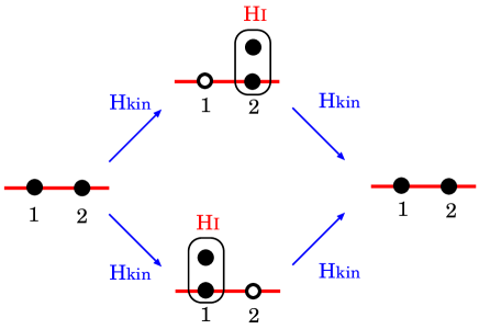
Figure 1: (Color online) The second-order process with $H_{\rm kin}$. In the initial and final states, one hole sits at site 1 and another sits at site 2. In the intermediate state, two holes are on the same site, where the Coulomb interaction works.

We start by one hole sitting at site 1 and another at site 2, and carry out the second-order perturbation calculation, as illustrated in Fig. 1. The transfer integral between $xy$ orbitals in the nearest-neighbor sites may be generally different from those between $yz$ orbitals and between $zx$ orbitals, since the orbitals are defined in the local coordinate frames. Nevertheless we assume them to be a same value, which is denoted as $t_{1}$, since the difference merely gives rise to minor corrections to the values of $J^{\prime}_{z}$ and $J^{\prime}_{xy}$ in Eqs. (9) and (10).

In the intermediate state, we take full account of the Coulomb interaction between two holes. We numerically evaluate the second-order energy given in a $4\times 4$ matrix form. This matrix is expressed in terms of the spin operators ${\bf S}$ acting on the doublet. It is given by

$$H(1,2)=C+H^{(0)}(1,2)+H_{z}^{(1)}(1,2)+H_{xy}^{(1)}(1,2),$$ (7)

with

$$H^{(0)}(1,2) = J_{\rm ex}{\bf S}_{1}\cdot{\bf S}_{2},$$ (8)

$$H_{z}^{(1)}(1,2) = J^{\prime}_{z}S_{1}^{z}S_{2}^{z},$$ (9)

$$H_{xy}^{(1)}(1,2) = \textrm{sgn}(1,2)J^{\prime}_{xy}\left(S_{1}^{x}S_{2}^{x}-S_{1}^{y}S_{2}^{y}\right),$$ (10)

where $\textrm{sgn}(i,j)$ gives $+1(-1)$ when the bond between the sites $i$ and $j$ is along the $x$ ($y$) axis, and $C$ is a constant. Table 1 shows the calculated coupling constants for various parameter sets of the Hubbard model. Both $J^{\prime}_{z}$ and $J^{\prime}_{xy}$ vanish without Hund’s coupling $J$ because we can check they are proportional to $J$. Note that $J^{\prime}_{z}$ is negative and its absolute value is nearly the same as $J^{\prime}_{xy}$ within the significant figures. These tendencies are consistent with the previous study. Jackeli and Khaliullin (2009); Kim et al. (2012a)

Table 1: Exchange couplings for various parameter sets, in units of eV. The transfer integral and the spin-orbit coupling are fixed at $t_{1}=0.36$ and $\zeta_{\rm SO}=0.36$.

$U$	$U^{\prime}$	$J$	$J_{\rm ex}$	$J^{\prime}_{\rm z}$	$J^{\prime}_{\rm xy}$
$1.4$	$1.4$	$0$	$0.165$	$0$	$0$
$1.4$	$0.98$	$0.21$	$0.223$	$-0.0055$	$0.0055$
$2.2$	$2.2$	$0$	$0.105$	$0$	$0$
$2.2$	$1.78$	$0.21$	$0.124$	$-0.0023$	$0.0023$
$2.2$	$1.54$	$0.33$	$0.144$	$-0.0046$	$0.0046$
$3.0$	$3.0$	$0$	$0.077$	$0$	$0$
$3.0$	$2.34$	$0.33$	$0.095$	$-0.0023$	$0.0023$
$3.0$	$2.1$	$0.45$	$0.107$	$-0.0039$	$0.0039$

III Excitation Spectra

As a next step to the analysis of the preceding section, we consider the following spin Hamiltonian in the square lattice:

$$H=H^{(0)}+H^{(1)},$$ (11)

with

$$H^{(0)} = \sum_{\langle i,j\rangle}H^{(0)}(i,j),$$ (12)

$$H^{(1)} = \sum_{\langle i,j\rangle}H_{z}^{(1)}(i,j)+H_{xy}^{(1)}(i,j).$$ (13)

The ground state takes the conventional antiferromagnetic spin configuration in the absence of the anisotropic term $H^{(1)}$. The direction of the staggered moment is not determined. The $H_{z}^{(1)}$ makes the direction favor the the $xy$ plane when $J^{\prime}_{z}<0$. This antiferromagnetic order breaks the rotational invariance of the isospin space in the $ab$ plane. We assume the staggered moment pointing to the $x$ axis.Cao et al. (1998) It should be noted here that the antiferromagnetic order in the local coordinate frames indicates the presence of the weak ferromagnetic moment in the global coordinate frame. Labeling the $x$, $y$, and $z$ axes as $z^{\prime}$, $x^{\prime}$, and $y^{\prime}$ axes, respectively, we express the spin operators by boson operators within the lowest order of $1/S$-expansion:Holstein and Primakoff (1940)

$$S_{i}^{z^{\prime}} = S-a_{i}^{\dagger}a_{i},\quad S_{i}^{x^{\prime}}+iS_{i}^{y^{\prime}}=\sqrt{2S}a_{i},$$ (14)

$$S_{j}^{z^{\prime}} = -S+b_{j}^{\dagger}b_{j},\quad S_{j}^{x^{\prime}}+iS_{j}^{y^{\prime}}=\sqrt{2S}b_{j}^{\dagger},$$ (15)

where $a_{i}$ and $b_{j}$ are boson annihilation operators, and $i$ ($j$) refers to sites on the A (B) sublattice. Using Eqs. (14) and (15), $H^{(0)}$ and $H^{(1)}$ may be expressed as

$$H^{(0)} = J_{\rm ex}S\sum_{\langle i,j\rangle}(a_{i}^{\dagger}a_{i}+b^{\dagger}_{j}b_{j}+a_{i}b_{j}+a_{i}^{\dagger}b_{j}^{\dagger}),$$ (16)

$$H^{(1)} = J^{\prime}_{z}S\frac{1}{2}\sum_{\langle i,j\rangle}(a_{i}-a_{i}^{\dagger})(b_{j}-b_{j}^{\dagger})$$ (17)

$$+ J^{\prime}_{xy}S\sum_{\langle i,j\rangle}\textrm{sgn}(i,j)(a_{i}^{\dagger}a_{i}+b_{j}^{\dagger}b_{j})$$

$$- J^{\prime}_{xy}S\frac{1}{2}\sum_{\langle i,j\rangle}\textrm{sgn}(i,j)(a_{i}+a_{i}^{\dagger})(b_{j}^{\dagger}+b_{j}).$$

where the unimportant constant term is neglected. The second term in Eq. (17) is canceled out by the factor $\pm$. Then we introduce the Fourier transforms of the boson operators in the magnetic Brillouin zone,

$$a({\bf k}) = \sqrt{\frac{2}{N}}\sum_{i}a_{i}\exp(-i{\bf k}\cdot{\bf r}_{i}),$$ (18)

$$b({\bf k}) = \sqrt{\frac{2}{N}}\sum_{j}b_{j}\exp(-i{\bf k}\cdot{\bf r}_{j}),$$ (19)

where $N$ is the number of sites, and $i$ ($j$) runs over A (B) sublattice. We obtain

$$H^{(0)} = J_{\rm ex}Sz\sum_{\bf k}a^{\dagger}({\bf k})a({\bf k})+b^{\dagger}({\bf k})b({\bf k})$$ (20)

$$+ \gamma({\bf k})[a^{\dagger}({\bf k})b^{\dagger}({\bf-k})+a({\bf k})b({\bf-k})],$$

$$H_{z}^{(1)} = J^{\prime}_{z}(2S)\sum_{\bf k}\gamma({\bf k})[a({\bf k})-a^{\dagger}({\bf-k})][b({\bf-k})-b^{\dagger}({\bf k})],$$

$$H_{xy}^{(1)} = -J^{\prime}_{xy}(2S)\sum_{\bf k}\eta({\bf k})[a({\bf k})+a^{\dagger}({\bf-k})][b({\bf-k})+b^{\dagger}({\bf k})],$$

where

$$\gamma({\bf k}) = \frac{1}{2}(\cos k_{x}+\cos k_{y}),$$ (23)

$$\eta({\bf k}) = \frac{1}{2}(\cos k_{x}-\cos k_{y}).$$ (24)

Here $z$ is the number of nearest neighbors, i.e., $z=4$.

To find out the excitation modes, we introduce the Green’s functions,

$$G_{aa}({\bf k},t) = -i\langle T[a({\bf k},t)a^{\dagger}({\bf k},0)]\rangle,$$ (25)

$$F_{ba}({\bf k},t) = -i\langle T[b^{\dagger}({\bf-k},t)a^{\dagger}({\bf k},0)]\rangle,$$ (26)

$$G_{ba}({\bf k},t) = -i\langle T[b({\bf k},t)a^{\dagger}({\bf k},0)]\rangle,$$ (27)

$$F_{aa}({\bf k},t) = -i\langle T[a^{\dagger}({\bf-k},t)a^{\dagger}({\bf k},0)]\rangle,$$ (28)

where $T$ is the time ordering operators, and $\langle X\rangle$ denotes the ground-state average of operator $X$. The $F_{ba}({\bf k},t)$ and $F_{aa}({\bf k},t)$ belong to the so called anomalous type. Defining their Fourier transforms by $G_{aa}({\bf k},\omega)=\int G_{aa}({\bf k},t){\rm e}^{i\omega t}{\rm d}t$ and so on, we derive the equation of motion for these functions,

$$\left(\begin{array}[]{cccc}\omega-1&-A({\bf k})&B({\bf k})&0\\ -A({\bf k})&-(\omega+1)&0&B({\bf k})\\ B({\bf k})&0&\omega-1&-A({\bf k})\\ 0&B({\bf k})&-A({\bf k})&-(\omega+1)\end{array}\right)$$ (33)

$$\times \left(\begin{array}[]{c}G_{aa}({\bf k},\omega)\\ F_{ba}({\bf k},\omega)\\ G_{ba}({\bf k},\omega)\\ F_{aa}({\bf k},\omega)\end{array}\right)=\left(\begin{array}[]{c}1\\ 0\\ 0\\ 0\end{array}\right),$$ (42)

where

$$A({\bf k}) = (1+g_{z})\gamma({\bf k})-g_{xy}\eta({\bf k}),$$ (43)

$$B({\bf k}) = g_{z}\gamma({\bf k})+g_{xy}\eta({\bf k}),$$ (44)

$$g_{z} = J^{\prime}_{z}/(2J_{\rm ex}),\quad g_{xy}=J^{\prime}_{xy}/(2J_{\rm ex}).$$ (45)

Here the energy is measured in units of $J_{\rm ex}Sz$. Hence we finally obtain,

$$\left(\begin{array}[]{c}G_{aa}({\bf k},\omega)\\ F_{ba}({\bf k},\omega)\\ G_{ba}({\bf k},\omega)\\ F_{aa}({\bf k},\omega)\\ \end{array}\right)=\frac{1}{D({\bf k},\omega)}\left(\begin{array}[]{c}g_{aa}({\bf k},\omega)\\ f_{ba}({\bf k},\omega)\\ g_{ba}({\bf k},\omega)\\ f_{aa}({\bf k},\omega)\\ \end{array}\right),$$ (46)

where

$$D({\bf k},\omega) = \omega^{4}-2[1+B({\bf k})^{2}-A({\bf k})^{2}]\omega^{2}+1-2A({\bf k})^{2}$$ (47)

$$- 2B({\bf k})^{2}+[A({\bf k})^{2}-B({\bf k})^{2}]^{2},$$

$$g_{aa}({\bf k},\omega) = (\omega-1)(\omega+1)^{2}-B({\bf k})^{2}(\omega-1)$$ (48)

$$+ A({\bf k})^{2}(\omega+1),$$

$$f_{ba}({\bf k},\omega) = -A({\bf k})[(\omega^{2}-1)-B({\bf k})^{2}+A({\bf k})^{2}],$$ (49)

$$g_{ba}({\bf k},\omega) = B({\bf k})[B({\bf k})^{2}-(\omega+1)^{2}-A({\bf k})^{2}],$$ (50)

$$f_{aa}({\bf k},\omega) = 2A({\bf k})B({\bf k}).$$ (51)

In the absence of the anisotropic terms, we have $A({\bf k})=\gamma({\bf k})$ and $B({\bf k})=0$. Inserting these relations into Eqs. (47)-(51), we have

$$G_{aa}({\bf k},\omega) = \frac{\omega+1}{\omega^{2}-(1-\gamma({\bf k})^{2})},$$ (52)

$$F_{ba}({\bf k},\omega) = -\frac{\gamma({\bf k})}{\omega^{2}-(1-\gamma({\bf k})^{2})},$$ (53)

$$G_{ba}({\bf k},\omega) = F_{aa}({\bf k},\omega)=0.$$ (54)

These forms are well-known for the isotropic Heisenberg model.Bulut et al. (1989)

In the presence of the anisotropic terms, Eq. (47) is rewritten as

$$D(\textbf{k},\omega)=[\omega^{2}-E_{-}^{2}(\textbf{k})][\omega^{2}-E_{+}^{2}(\textbf{k})],$$ (55)

with

$$E_{\pm}(\textbf{k})=\sqrt{[1\pm|B(\textbf{k})|]^{2}-A^{2}(\textbf{k})}.$$ (56)

This indicates that poles exist at $\omega=E_{\pm}({\bf k})$ in the domain of $\omega>0$. To clarify the behavior of the poles, we express the Green’s function as

$$G_{aa}(\textbf{k},\omega)=\frac{1}{2}\left[\frac{\omega+1+|B(\textbf{k})|}{\omega^{2}-E_{+}^{2}(\textbf{k})}+\frac{\omega+1-|B(\textbf{k})|}{\omega^{2}-E_{-}^{2}(\textbf{k})}\right].$$ (57)

This form indicates that two poles have nearly equal weights in the domain of $\omega>0$ in the case of weak anisotropic terms. At the $\Gamma$-point, $A({\bf k})=1+g_{z}$ and $B({\bf k})=g_{z}$, and hence $D(0,\omega)$ $=$ $\omega^{2}(\omega^{2}+4g_{z})$. Therefore one mode has zero excitation energy while the other has a finite energy $2\sqrt{-g_{z}}$. The former may correspond to the Goldstone mode due to breaking the rotational invariance of the isospin in the $ab$ plane. At the X-point, ${\bf k}=(\pi,0)$, $A({\bf k})=$ $-B({\bf k})$ $=g_{xy}$, and hence the two modes have excitation energies $\omega=\sqrt{1\pm 2g_{xy}}$. At the M-point, since $A({\bf k})=$ $B({\bf k})=0$, the two modes have the same excitation energy, $\omega=1$.

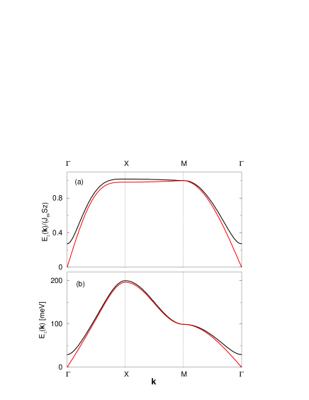
Figure 2: (Color online) Excitation energies of two modes $E_{\pm}(\textbf{k})$ as a function of ${\bf k}$ along the symmetry lines. (a) $E_{\pm}(\textbf{k})$ evaluated from Eq. (56). The parameters are evaluated from the Hubbard model with $t_{1}=0.36$ eV, $\zeta_{\rm SO}=0.36$ eV, $U=3.0$ eV, $U^{\prime}=2.1$ eV, and $J=0.45$ eV with $g_{z}=-0.018$ and $g_{xy}=0.018$ in units of $J_{\rm ex}Sz$. (b) $E_{\pm}(\textbf{k})$ evaluated from Eq. (62) including $J_{\textrm{ex}}^{\prime}/J_{\textrm{ex}}=-1/3$ and $J_{\textrm{ex}}^{\prime\prime}/J_{\textrm{ex}}=1/4$ with $J_{\textrm{ex}}=59$ meV. The parameters are evaluated from the Hubbard model with $t_{1}=0.3$ eV, $\zeta_{\rm SO}=0.4$ eV, $U=3.5$ eV, $U^{\prime}=2.6$ eV, and $J=0.45$ eV with $g_{z}=-0.015$ and $g_{xy}=0.015$ in units of $J_{\rm ex}Sz$.

Figure 2 shows the dispersion relation along the symmetry lines of ${\bf k}$ for $g_{z}=-0.018$ and $g_{xy}=0.018$. The parameters correspond to the Hubbard model with $t_{1}=0.36$ eV, $\zeta_{\rm SO}=0.36$ eV, $U=3.0$ eV, $U^{\prime}=2.1$ eV, and $J=0.45$ eV (last row in Table 1). Although $J^{\prime}_{z}$ and $J^{\prime}_{xy}$ are two orders of magnitude smaller than $J_{\rm ex}$, they substantially modify the dispersion relation. Note that $J_{\rm ex}Sz(\equiv 2J_{\rm ex})=0.214$ eV, which is comparable to the excitation energy at the X-point observed in resonant inelastic x-ray scattering (RIXS) at the $L$-edge of Ir.Kim et al. (2012b)

Finally, let us consider what happens when the exchange interactions between the second and third neighbor sites, denoted as $J_{\textrm{ex}}^{\prime}$ and $J_{\textrm{ex}}^{\prime\prime}$ respectively, are introduced in addition to $J_{\textrm{ex}}$. It is known that a phenomenological isotropic model constructed by $J_{\textrm{ex}}$, $J_{\textrm{ex}}^{\prime}$, and $J_{\textrm{ex}}^{\prime\prime}$ couplings gives much better dispersion curve.Kim et al. (2012b) We expect the inclusion of $J_{\textrm{ex}}^{\prime}$ and $J_{\textrm{ex}}^{\prime\prime}$ terms improves the dispersion curve in comparison with the experimental one since the contributions from the anisotropic terms are not so significant in the wide range of the Brillouin zone as shown in Fig. 2 (a). Then, our concern is whether or not the gap between the two modes around the $\Gamma$ point remains finite quantitatively. We see the answer is in the affirmative as follows.

In the presence of $J_{\textrm{ex}}^{\prime}$ and $J_{\textrm{ex}}^{\prime\prime}$ terms, the coefficient matrix appeared in Eq. (42) is modified as

$$\left(\begin{array}[]{cccc}\omega-1+\xi(\textbf{k})&-A({\bf k})&B({\bf k})&0\\ -A({\bf k})&-(\omega+1-\xi(\textbf{k}))&0&B({\bf k})\\ B({\bf k})&0&\omega-1+\xi(\textbf{k})&-A({\bf k})\\ 0&B({\bf k})&-A({\bf k})&-(\omega+1-\xi(\textbf{k}))\end{array}\right),$$ (58)

where

$$\xi(\textbf{k}) = \frac{J_{\textrm{ex}}^{\prime}}{J_{\textrm{ex}}}(1-\gamma^{\prime}(\textbf{k}))+\frac{J_{\textrm{ex}}^{\prime\prime}}{J_{\textrm{ex}}}(1-\gamma^{\prime\prime}(\textbf{k})),$$ (59)

$$\gamma^{\prime}(\textbf{k}) = \cos k_{x}\cos k_{y},$$ (60)

$$\gamma^{\prime\prime}(\textbf{k}) = \frac{1}{2}[\cos(2k_{x})+\cos(2k_{y})].$$ (61)

Then, the excitation energies for two modes become

$$E_{\pm}(\textbf{k})=\sqrt{[1-\xi(\textbf{k})\pm|B(\textbf{k})|]^{2}-A^{2}(\textbf{k})}.$$ (62)

Since the extra term $\xi(\textbf{k})$ goes to zero when $|\textbf{k}|\rightarrow 0$, the existence of the gap of the two modes at the $\Gamma$ point is robust.

The experimental dispersion curve can be reproduced well by setting $J_{\textrm{ex}}=60$ meV, $J_{\textrm{ex}}^{\prime}=-J_{\textbf{ex}}/3$ and $J_{\textrm{ex}}^{\prime\prime}=J_{\textbf{ex}}/4$ in the phenomenological model without the anisotropic terms $J_{z}^{\prime}$ and $J_{xy}^{\prime}$.Kim et al. (2012b) With the parameter set of $U=3.5$ eV, $U^{\prime}=2.6$ eV, $J=0.45$ eV, $t_{1}=0.3$ eV, and $\zeta_{\textrm{SO}}=0.4$ eV, we obtain $J_{\textrm{ex}}\simeq 60$ meV, $J_{xy}^{\prime}=-J_{z}^{\prime}=1.8$ meV. Together with the relations $J_{\textrm{ex}}^{\prime}=-J_{\textbf{ex}}/3$ and $J_{\textrm{ex}}^{\prime\prime}=J_{\textbf{ex}}/4$, the $E_{\pm}(\textbf{K})$ can be numerically evaluated. As shown in Fig. 2 (b), the inclusion of $J_{\textrm{ex}}^{\prime}$ and $J_{\textrm{ex}}^{\prime\prime}$ improves the dispersion curve as expected. On the other hand, the splitting of the two modes, which is the most prominent around the $\Gamma$ point, remains nearly intact and the magnitude of the gap keeps nearly the same order of magnitude as that obtained for the parameter set evaluated in the absence of $J_{\textrm{ex}}^{\prime}$ and $J_{\textrm{ex}}^{\prime\prime}$.

IV Concluding remarks

We have studied the low-lying excitations in Sr₂IrO₄ on the localized electron picture. Having introduced the isospin operators acting on Kramers’ doublet, we have derived the effective spin Hamiltonian from the multi-orbital Hubbard model by the second-order perturbation with the electron transfer. This approach may be justified in the strong Coulomb interaction. It consists of the isotropic Heisenberg term and small anisotropic terms. Expanding the spin operators in terms of boson operators, we have introduced the Green’s functions for the boson operators, and have solved the coupled equations of motion for those functions. The excitation spectra have been obtained from the Green’s functions. It is found that two modes emerge with slightly different energies due to the anisotropic terms, in contrast to the spin waves in the isotropic Heisenberg model.

The existence of the anisotropic terms, which is the hallmark of the interplay between the SOI and the Coulomb interaction, has not been corroborated by experiments.Kim et al. (2012b); Fujiyama et al. (2012) The magnetic excitations are usually detected by the inelastic neutron scattering, but it may be hard for the present system due to the strong absorption of neutron by Ir atom. Recently, the spin and orbital excitations have been observed and analyzed by the Ir $L$-edge RIXS. No indication of the splitting is unfortunately found in the spectral shape.Kim et al. (2012b); Ament et al. (2011) Since the energy difference is around $60$ meV at most, it may be difficult to distinguish the two modes by the RIXS experiments. However, the observation with finer instrumental energy resolution of 36 meV may be within the reach at the $L_{2,3}$ edges of Ir.Sala et al. (2013)

Finally we comment on the validity of the strong coupling approach. The excitation energy at the M point is the same as at the X point within the nearest-neighbor coupling in the Heisenberg model. Since the energy at the M point is found nearly the half of that at the X point in the RIXS, we need to include the next-nearest-neighbor coupling as large as one third of the nearest neighbor coupling to account for such difference.Kim et al. (2012b) In addition, the Mott-Hubbard gap is estimated as $\sim 0.4$ eV from the optical absorption spectra,Kim et al. (2008); Moon et al. (2009) which value is comparable to the magnetic excitation energy $2J\sim 0.2$ eV. These indicate that the strong coupling approach may not work well. It may be interesting to study the elementary excitations from the viewpoint of the itinerant electron picture workable in the weak and intermediate couplings.

References

• Crawford et al. (1994) M. K. Crawford, M. A. Subramanian, R. L. Harlow, J. A. Fernandez-Baca, Z. R. Wang, and D. C. Johnston, Phys. Rev. B 49, 9198 (1994).
• Cao et al. (1998) G. Cao, J. Bolivar, S. McCall, J. E. Crow, and R. P. Guertin, Phys. Rev. B 57, R11039 (1998).
• Moon et al. (2006) S. J. Moon, M. W. Kim, K. W. Kim, Y. S. Lee, J.-Y. Kim, J.-H. Park, B. J. Kim, S.-J. Oh, S. Nakatsuji, Y. Maeno, et al., Phys. Rev. B 74, 113104 (2006).
• Kim et al. (2008) B. J. Kim, H. Jin, S. J. Moon, J.-Y. Kim, B.-G. Park, C. S. Leem, J. Yu, T. W. Noh, C. Kim, S.-J. Oh, et al., Phys. Rev. Lett. 101, 076402 (2008).
• Arita et al. (2012) R. Arita, J. Kuneš, A. V. Kozhevnikov, A. G. Eguiluz, and M. Imada, Phys. Rev. Lett. 108, 086403 (2012).
• Watanabe et al. (2010) H. Watanabe, T. Shirakawa, and S. Yunoki, Phys. Rev. Lett. 105, 216410 (2010).
• Kim et al. (2009) B. J. Kim, H. Ohsumi, T. Komesu, S. Sakai, T. Morita, H. Takagi, and T. Arima, Science 323, 1329 (2009).
• Jackeli and Khaliullin (2009) G. Jackeli and G. Khaliullin, Phys. Rev. Lett. 102, 017205 (2009).
• Jin et al. (2009) H. Jin, H. Jeong, T. Ozaki, and J. Yu, Phys. Rev. B 80, 075112 (2009).
• Kim et al. (2012a) B. H. Kim, G. Khaliullin, and B. I. Min, Phys. Rev. Lett. 109, 167205 (2012a).
• Wang and Senthil (2011) F. Wang and T. Senthil, Phys. Rev. Lett. 106, 136402 (2011).
• Holstein and Primakoff (1940) T. Holstein and H. Primakoff, Phys. Rev. 58, 1098 (1940).
• Bulut et al. (1989) N. Bulut, D. Hone, D. J. Scalapino, and E. Y. Loh, Phys. Rev. Lett. 62, 2192 (1989).
• Kanamori (1963) J. Kanamori, Prog. Theor. Phys. 30, 275 (1963).
• Kim et al. (2012b) J. Kim, D. Casa, M. H. Upton, T. Gog, Y.-J. Kim, J. F. Mitchell, M. van Veenendaal, M. Daghofer, J. van den Brink, G. Khaliullin, et al., Phys. Rev. Lett. 108, 177003 (2012b).
• Fujiyama et al. (2012) S. Fujiyama, H. Ohsumi, T. Komesu, J. Matsuno, B. J. Kim, M. Takata, T. Arima, and H. Takagi, Phys. Rev. Lett. 108, 247212 (2012).
• Ament et al. (2011) L. J. P. Ament, G. Khaliullin, and J. van den Brink, Phys. Rev. B 84, 020403 (2011).
• Sala et al. (2013) M. M. Sala, C. Henriquet, L. Simonelli, R. Verbeni, and G. Monaco, J. Electron Spectrosc. Relat. Phenom. 188, 150 (2013).
• Moon et al. (2009) S. J. Moon, H. Jin, W. S. Choi, J. S. Lee, S. S. A. Seo, J. Yu, G. Cao, T. W. Noh, and Y. S. Lee, Phys. Rev. B 80, 195110 (2009).