Abstract

We consider the problem of estimating a continuous distribution function $F$, as well as meaningful functions $\tau(F)$ under a large class of loss functions. We obtain best invariant estimators and establish their minimaxity for Hölder continuous $\tau$’s and strict bowl-shaped losses with a bounded derivative. We also introduce and motivate the use of integrated balanced loss functions which combine the criteria of an integrated distance between a decision $d$ and $F$, with the proximity of $d$ with a target estimator $d_{0}$. Moreover, we show how the risk analysis of procedures under such an integrated balanced loss relates to a dual risk analysis under an “unbalanced” loss, and we derive best invariant estimators, minimax estimators, risk comparisons, dominance and inadmissibility results. Finally, we expand on various illustrations and applications relative to maxima-nomination sampling, median-nomination sampling, and a case study related to bilirubin levels in the blood of babies suffering from jaundice.

Keywords: Balanced loss; best invariant estimator; cumulative distribution function; inadmissibility; integrated loss; maxima-nomination sampling; median-nomination sampling; minimax; nonparametric estimation; risk function; strict bowl-shaped loss.

AMS 2010 Subject Classification: Primary: 62C20; Secondary: 62G05

1 Introduction

An appealing and wide ranging formulation for estimating a continuous distribution function (cdf) $F$ based on $X=(X_{1},\ldots,X_{n})$, where $X_{i}$’s are independently and identically distributed (i.i.d.) on $I=(a,b)\subseteq\mathbb{R}$ with cdf $F$, is to measure the discrepancy between an estimate $d(\cdot):\mathbb{R}\to[0,1]$ and $F$ as

$$\int_{\mathbb{R}}\,\rho(d(t)-F(t))\,H(F(t))\,dF(t)\,,$$ (1)

where $\rho$ is strictly bowl-shaped on its domain with $\rho(0)=0$, $\rho^{\prime}(z)<0$ for $z<0$, $\rho^{\prime}(z)>0$ for $z>0$, and $H$ is a continuous and positive weight function. Aggarwal (1955) introduced such a formulation for Cramér-von Mises loss with $\rho(z)=|z|^{r}$; $r\in\{1,2,\ldots\}$, considered an invariance structure relative to the group of continuous and strictly increasing transformations, and obtained best invariant estimators of $F$. For instance, the empirical distribution function $F_{n}$ is the best invariant estimator of $F$ under loss (1) with $\rho(z)=z^{2}$ and $H(z)=(z(1-z))^{-1}$ (e.g., Ferguson, 1967, Section 4.8). Now, in terms of the larger class of (not necessarily invariant) procedures, challenging issues with regards to the potential minimaxity and admissibility of the best invariant procedure have been addressed by Dvoretzky et al. (1956), Phadia (1973), Cohen and Kuo (1985), Brown (1988), Yu (1989), and Yu and Chow (1991). Namely, Yu (1992) established the minimaxity of the best invariant procedure in Aggarwal’s setup and analog minimaxity findings have been obtained by Mohammadi and van Zwet (2002, entropy loss), Ning and Xie (2007, Linex loss), and Stępień-Baran (2010, strictly convex $\rho$). Parallel developments for the alternative Kolmogorov-Smirnov loss $\sup_{t\in\mathbb{R}}|d(t)-F(t)|$ were given by Brown (1988), Friedman et al. (1988), and Yu and Phadia (1992).

In this paper, we seek to extend Stępień-Baran’s minimax result to loss functions of the form

$$L_{\rho,\tau}(d,F)\,=\,\int_{\mathbb{R}}\,\rho(\tau(d(t))-\tau(F(t)))\,dF(t)\,,$$ (2)

with $\rho$ strict bowl-shaped, differentiable almost everywhere (a.e.), and with $\tau(\cdot)$ a continuous and strictly monotone function on $[0,1]$.

A first motivation here is to provide analytical results applicable to non-strict convex choices of $\rho$ which are not covered by previous findings even for identity $\tau$. As well, the loss functions in (2) are flexible enough to include loss functions of the form

$$\int_{\mathbb{R}}\,\rho_{0}(\frac{d(t)}{F(t)})\,dF(t)\,,$$ (3)

contrasting directly the ratios $\frac{d(t)}{F(t)}$, as opposed to the differences $d(t)-F(t)$, with $\rho\equiv\rho_{0}\circ\log$, and $\rho_{0}$ strict bowl-shaped. Notice here that the strict bowl-shapedness of $\rho$ and $\rho_{0}$ are equivalent, which is not the case as for convexity. An example of (3) is the integrated entropy loss with $\rho_{0}(z)=z^{-1}+\log(z)-1$, (see Mohammadi and van Zwet, 2002). The losses in (2) also encompass integrated $L^{2}$ losses of the form

$$L_{\tau}(d,F)=\int_{\mathbb{R}}\big{(}\tau(d(t))-\tau(F(t))\big{)}^{2}dF(t),$$ (4)

which correspond of course to $\rho(z)=z^{2}$ in (2). An interesting example of (4) is the so-called precautionary loss function with $\tau(z)=e^{az}$; $a\neq 0$; which is nicely motivated from a practical point of view (e.g., Schäbe, 1991; Norstrøm, 1996). For more examples see Jafari Jozani and Marchand (2007).

Another motivation to study integrated losses of the form (2) with non-identity $\tau$ resides in the equivalence of the performances of estimates $d(\cdot)$ of $F$ under loss (2) with estimates $d^{*}(\cdot)\equiv\tau(d(\cdot))$ of $\tau(F)$ under loss

$$\int_{\mathbb{R}}\,\rho(d^{*}(t)-\tau(F(t)))\,dF(t)\,.$$ (5)

Although the problems are mathematically equivalent, they emanate from different practical perspectives. Indeed, for the latter problem, our interest lies in estimating a meaningful function $\tau(F(t)),t\in\mathbb{R}$, such as a logarithmic function $\log(1+z)$, polynomials $z^{m}$ and $1-(1-z)^{m}$ representing for instance the cdf’s of the minimum and maximum of $m$ independent copies generated from $F$, and similarly $z^{1/k}$ and $1-(1-z)^{1/k}$ arising in maxima or minima nomination samples when the set size is an integer $k\geq 1$ (e.g., Wells and Tiwari, 1990). Other interesting choices, further discussed in Examples 2, 3, and 4, are the odds-ratio $\tau(z)=\frac{z}{1-z}$ and the log odds-ratio $\tau(z)=\log(\frac{z}{1-z})$. However, even in cases where a best invariant estimator exists, these choices will not satisfy a Hölder continuity condition on $\tau$ that is required for the minimaxity of the best invariant estimator to follow from our Theorem 2.

In Section 2.1, we provide preliminary results and examples for the best invariant estimator, expand on issues related to the role of the action space, the presence of best invariant solutions which are not genuine cdf’s, and corresponding adjustments which we present as best constrained invariant estimators of $F$ and $\tau(F)$ (Remark 3). In Section 2.2, we pursue with a general minimax result (Theorem 2). To this end, we exploit a key result from Yu and Chow (1991), we require $\rho$ to have a bounded derivative, and we work with a Hölder continuity assumption for $\tau$. This minimax result can be viewed as an extension of Stępień-Baran’s (2010) minimax result to losses $L_{\rho,\tau}(d,F)$ with either strict bowl-shaped $\rho$ and/or non-identity $\tau$. We also point out (Theorem 3) that the best invariant and minimax properties are preserved for a class of weighted integrated loss functions, which will play a critical role in Section 3.

In Section 3, as an alternative, we propose and motivate the use of an integrated balanced loss function in the spirit of Jafari Jozani, Marchand and Parsian (2006). This loss function, presented in the context of estimating $\tau(F)$, is of the form

$$L_{\omega,d_{0}}(d,F)=\int_{\mathbb{R}}\{w(x,t)(d(t)-d_{0}(t))^{2}+(1-w(x,t))(d(t)-\tau(F(t))^{2}\}\,dF(t)\,$$

with $d_{0}$ being the target estimator of $\tau(F)$, and $w(\cdot,\cdot)\in[0,1]$ is a data dependent weight function which permits one to combine the criteria that the estimate $d(\cdot)$ be close to the target estimator $d_{0}(\cdot)$ (which can be chosen for instance as $\tau(F_{n})$, with $F_{n}$ being the empirical cdf) with integrated squared error $L_{\tau}(\tau^{-1}(d),F)$ as in (4). We describe explicitly how the performance of estimators of $\tau(F)$ under loss $L_{\omega,d_{0}}$ relates to the performance of a dual estimator of $\tau(F)$ under “unbalanced” loss $L_{\omega,d_{0}}$ with $\omega\equiv 0$. This leads to the determination of the best invariant estimator (Theorem 4), as well as a proof of its minimaxity (Theorem 5) among all estimators for cases where both $w$ and $d_{0}$ satisfy an invariance requirement (i.e., being functions of the $X_{i}$’s only through their order statistics). Moreover, the same duality between the “balanced” and “unbalanced” cases, along with known results for the “unbalanced” case leads to dominance and inadmissibility results (Theorem 6). We advocate the use of such balanced integrated losses to provide a flexible and natural tool for estimating $F$. In particular, it permits us to set the weight $w(x,t)$ equal to $1$ whenever $F_{n}(t)$ takes the values $0$ or $1$, leading to a best invariant (and minimax) estimator that is a genuine cdf.

Section 4 is devoted to applications and illustrations relative to maxima-nomination sampling and median-nomination sampling. In Section 5, an actual data set, pertaining to bilirubin levels in the blood of babies suffering from jaundice, is analyzed via an integrated balanced loss function. In Section 6, we provide some concluding remarks. Finally, the proofs and further complementary developments with respect to balanced loss functions are presented in the Appendix.

2 Best invariant and minimax estimators of $F$ and $\tau(F)$

2.1 Preliminary results and the best invariant estimator

Let $\textbf{X}=(X_{1},\ldots,X_{n})$ be a random sample of size $n\geq 2$ from an unknown continuous distribution function $F$ supported on $(a,b)$, and denote its associated order statistics by $\textbf{Y}=(Y_{1},\ldots,Y_{n})$. Define also $Y_{0}=a$ and $Y_{n+1}=b$. Let $\mathcal{A}=\{d(\cdot):d(\cdot)$ is a nondecreasing function from $\mathbb{R}\text{ onto }[0,1]\}$ be the action space, and $\mathcal{F}=\{F:F$ is a continuous cumulative distribution function on $\mathbb{R}\}$ be the parameter space. Consider estimating $F$ under the integrated loss $L_{\rho,\tau}(d,F)$ in (2), $\rho$ strict bowl-shaped and differentiable a.e., and assume without loss of generality that $\tau$ is strictly increasing (otherwise, transform $\tau$ to $-\tau$). For an estimator $d(X;\cdot)$ of $F$, we define the corresponding frequentist risk as $R_{\rho,\tau}(d(X;\cdot),F)=E_{F}L_{\rho,\tau}(d(X;\cdot),F)$.

In his seminal paper, Aggarwal (1955) showed that, under the group of continuous and strictly increasing transformations, the class of invariant estimators considered here leads to estimators which are nondecreasing step functions with jumps at the observed order statistics, in other words, of the form

$$d(\textbf{Y};t)=\sum_{i=0}^{n}u_{i}\,\mathbb{I}(Y_{i}\leq t<Y_{i+1}),$$ (6)

for $t\in(a,b)$, where $0\leq u_{0}\leq\ldots\leq u_{n}\leq 1$, and $\mathbb{I}(B)$ denotes the indicator function of a set $B$. Our next results identify the best invariant estimator of $F$ in the current setup. Here and throughout, we set $T_{i}$, $i=0,\ldots,n$, to be random variables such that

$$T_{i}\sim\text{Beta}(i+1,n-i+1)\,,\;\hbox{ with pdf }f_{T_{i}}(\cdot)\,.$$

Theorem 1.

A best invariant estimator of $F$, whenever it exists, under loss $L_{\rho,\tau}(d,F)$ in (2), is given by $d^{*}(\textbf{Y};t)=\sum_{i=0}^{n}u^{*}_{i}\mathbb{I}(Y_{i}\leq t<Y_{i+1}),$ where $u^{*}_{i}$ is the Bayes point estimate of $p$ for the model $B|p\sim\hbox{Bin}(n,p)$, the observed $B=i$, the prior $p\sim U(0,1)$ (i.e., posterior for $p$ is $\text{Beta}(i+1,n-i+1)$), and loss $L(d,p)=\rho(\tau(d)-\tau(p))$. The risk of $d^{*}(\textbf{Y},t)$ is constant in $F$ and given by

$$R_{\rho,\tau}(d^{*},F)=\frac{1}{n+1}\;\sum_{i=0}^{n}\int_{0}^{1}\rho(\tau(u_{i}^{*})-\tau(t))\,f_{T_{i}}(t)\,dt,$$

where $0<u_{0}^{*}\leq\ldots\leq u_{n}^{*}<1.$

Proof.

The proof is given in Section 7.1. ∎

Remark 1.

A more general representation holds for Theorem 1 in the presence of a weight $H$ as in (1), with the $u_{i}^{*}$’s defined similarly but with a prior density on $p$ that is proportional to $H(p)$.

Remark 2.

Since $\tau$ is strictly monotone and continuous, a best invariant estimator of $\tau(F)$ under loss $L_{\rho,\tau}(\tau^{-1}(d),F)$ is given by $d^{*}_{\tau}(\textbf{Y};t)=\sum_{i=0}^{n}\tau(u^{*}_{i})\,\mathbb{I}(Y_{i}\leq t<Y_{i+1}),$ with the $u^{*}_{i}$’s given in Theorem 1.

For the particular case where $\rho(z)=z^{2}$ is squared error loss, since Bayes estimators are posterior expectations, the following specialization of Theorem 1 becomes immediately available.

Corollary 1.

1. A best invariant estimator of $\tau(F)$ under loss $L_{\tau}(\tau^{-1}(d),F)$ (see (4)), whenever it exists, is given by $d^{*}_{\tau}(\textbf{Y};t)=\sum_{i=0}^{n}u^{*}_{i,\tau}\mathbb{I}(Y_{i}\leq t<Y_{i+1})$, where $u^{*}_{i,\tau}=\tau(u^{*}_{i})=\mathbb{E}\big{[}\tau(T_{i})\big{]}$ for $i=0,\ldots,n$;

2. A best invariant estimator of $F$ under loss $L_{\tau}(d,F)$ in (4), whenever it exists, is given by $d^{*}(\textbf{Y};t)=\sum_{i=0}^{n}u^{*}_{i}\mathbb{I}(Y_{i}\leq t<Y_{i+1}),$ where

   $$u^{*}_{i}={\tau}^{-1}\big{(}\mathbb{E}\big{[}\tau(T_{i})\big{]}\big{)},\qquad\qquad\text{for }i=0,\ldots,n.$$ (7)

In both cases, the risk of the best invariant estimator is constant and given by $\frac{1}{n+1}\sum_{i=0}^{n}\mathbb{V}\text{ar}\big{[}\tau(T_{i})\big{]}.$

Example 1.

Corollary 1 applies to powers of $F$ with $\tau(z)=z^{m}$, $m>0$, and simply brings into play corresponding moments for Beta distributed $T_{i}$’s. For instance with $\rho(z)=z^{2}$, we obtain in Corollary 1

$$u_{i}^{*}=\{E({T_{i}}^{m}\,)\}^{1/m}=\left(\frac{(n+1)!\,\Gamma(i+m+1)}{i!\,\Gamma(n+m+2)}\right)^{1/m}\,,\,i=0,\ldots,n.$$ (8)

When $m=1$, a best invariant estimator of $F$ under loss (4) is obtained when $u_{i}^{*}=E(T_{i})=(i+1)/(n+2)$, a result first obtained by Aggarwal (1955).

Example 2.

(Odds and log-odds ratios) For the situation where $\tau(F)=\frac{F}{1-F}$ and $\rho(z)=|z|$ in (2), the risk of any invariant procedure is infinite as seen from (17) with $i=n$ and the divergence of $\int_{0}^{1}|\tau(u)-\frac{t}{1-t}|\,f_{T_{n}}(t)\,dF(t)$, for any $\tau(u)$. The same is true for $\rho$’s that are convex on $(0,\infty)$, such as for $L^{p}$ integrated losses with $\rho(z)=|z|^{p}$, $p>1$. Alternatively, concave $L^{p}$ choices with $0<p<1$ will lead to the existence of a best invariant estimator as can be verified by the convergence of (17) for all $i$, and with $\tau(u)=0$ (for instance). For estimating $\tau(F)=\log(\frac{F}{1-F})$, the best invariant procedures will exist in many more cases. In particular for $\rho(z)=z^{2}$, the best invariant procedures of Corollary 1 do exist with $u_{i,\tau}^{*}=E\left[\,\log(\frac{T_{i}}{1-T_{i}})\,\right]\,,$ and $u_{i}^{*}={e^{u_{i,\tau}^{*}}}/{(1+e^{u_{i,\tau}^{*}})};\;i=0,\ldots,n\,.$

Remark 3.

When $b<\infty$, all estimators of the form $\sum_{i=0}^{n}u_{i}\,\mathbb{I}(Y_{i}\leq t<Y_{i+1})+u_{n+1}\mathbb{I}(t\geq b)$, with fixed common $u_{0},\ldots,u_{n}$ and different $u_{n+1}$ are equivalent under loss (2). Hence, there are many best invariant estimators in the context of Theorem 1, and we can select $u_{n+1}=1$ so that best invariant estimates behave like a genuine cdf in the right tail. A similar situation applies when $a>-\infty$. When $a=-\infty$ and $b=+\infty$, the best invariant estimator is unique as given by Theorem 1.

A best invariant estimator of $F$ under loss $L_{\rho,\tau}(d,F)$ is always such that $u_{0}^{*}>0$ and $u_{n}^{*}<1$ (cf. Theorem 1). Along with the observations of the previous paragraph, this implies that $d^{*}$ can never be a genuine distribution function on the real line whenever $a=-\infty$ or $b=+\infty$. A simple way of overcoming such a difficulty is to force the invariant estimator of $F$ in  (6) to take the values $u_{0}^{*}=0$ and $u_{n}^{*}=1$. Said otherwise, one may work with the constrained action space $\mathcal{A}_{c}=\{d(\cdot):d\text{ is a distribution function on }\mathbb{R}\}.\,$ Since the minimization is performed for each step $i$, it is immediate that the best invariant estimator of $F$ for such a constrained problem under loss $L_{\rho,\tau}(d,F)$ is given by $d_{c}^{*}(\textbf{Y};t)=\sum_{i=1}^{n-1}u^{*}_{i}\,\mathbb{I}(Y_{i}\leq t<Y_{i+1})+\mathbb{I}(t\geq Y_{n})\,,$ where $u^{*}_{i}=\tau^{-1}\big{(}\mathbb{E}\big{[}\tau(T_{i})\big{]}\big{)}$, for $i=1,\ldots,n-1$.

Example 3.

(Example 2 continued) Revisiting Example 2 with $\tau(F)=\frac{F}{1-F}$ and $\rho(z)=|z|$, a constrained best invariant estimator of $F$ will exist, is derived from (18), leading to $u^{*}_{i}$ being the median of $T_{i}\sim\hbox{Beta}(i+1,n-i+1)$, for $i=1,\ldots,n-1$.

2.2 Minimaxity of the best invariant estimator

We now consider the minimaxity of the best invariant estimator $d^{*}$ introduced in Theorem 1 among all estimators in $\mathcal{A}$. To this end, we need the following useful lemma which establishes the existence of an invariant estimator $d_{0}$ and a cdf $F_{0}$ under which the behaviour of $d_{0}$ is arbitrarily close to that of a given $d\in A$.

Lemma 1.

(Yu and Chow, 1991, Theorem 4) Suppose that $d=d(\textbf{Y};t)$ is a nonrandomized estimator with finite risk and a measurable function of the order statistics Y. For any $s,\delta>0$ there exists a uniform distribution $P_{0}$ on a Lebesgue measurable subset $I\subseteq\mathbb{R}$ and an invariant estimator $d_{0}\in\mathcal{I}$ such that

$$P_{0}^{n+1}\{(\textbf{Y},t):|d(\textbf{Y};t)-d_{0}(\textbf{Y};t)|\geq s\}\leq\delta,$$

where $n\geq 2$ corresponds to the sample size.

The following result extends Theorem 2.2 of Yu (1992) and Theorem 1 of Stępień-Baran (2010) to the class of losses $L_{\rho,\tau}(d,F)$, when $\tau$ is Hölder continuous of order $\alpha\in(0,1]$, that is, there exists constants $\alpha,M>0$ such that

$$\big{|}\tau(t_{1})-\tau(t_{2})\big{|}\leq M\,\big{|}t_{1}-t_{2}\big{|}^{\alpha},$$

for all $t_{1},t_{2}\in[0,1]$. We write $\tau\in\mathcal{L}(\alpha)$ to denote this. Note that, under the Hölder continuity assumption for $\tau$ and the boundedness of $\rho$ on any finite interval, the risk of any invariant estimator is finite (hence a best invariant estimator will exist) as seen by Theorem 1’s representation (17).

Lemma 2.

Consider estimating $F$ under loss (2) with $\rho$ differentiable, strict-bowl shaped, $\rho^{\prime}$ bounded, and $\tau\in\mathcal{L}(\alpha)$ for $\alpha\in(0,1]$. Then, for any $d\in\mathcal{A}$ and $\epsilon>0$, there exists $F_{0}\in\mathcal{F}$ and $d_{0}\in\mathcal{I}$ such that $|R(d,F_{0})-R(d_{0},F_{0})|\leq\epsilon\,.$

Proof.

The proof is given in Section 7.2 ∎

What follows is our main minimaxity result.

Theorem 2.

For the problem of estimating $F$ under loss (2) with $\rho$ differentiable, strict-bowl shaped, $\rho^{\prime}$ bounded, and $\tau\in\mathcal{L}(\alpha)$ for $\alpha\in(0,1]$, the best invariant estimator $d^{*}$ is minimax, that is

$$\inf_{d\in\mathcal{A}}\sup_{F\in\mathcal{F}}R_{\tau}(d,F)=\sup_{F\in\mathcal{F}}R_{\tau}(d^{*},F).$$

Proof.

The proof is given in Section 7.3 ∎

Example 4.

As a continuation of Examples 1 and 2, we summarize how the results of this section apply or don’t apply. For log-odds ratios, although a best invariant estimator exists, the above minimaxity result does not apply since the function $\tau(z)=\log(\frac{z}{1-z})$ does not satisfy the Hölder continuity assumption. For powers $\tau(z)=z^{m}$ with $m>0$, we have Hölder continuity for $0<\alpha\leq m$ and the corresponding best invariant estimators of $F$ are minimax as long as $\rho$ satisfies the given conditions (examples include $L^{p}$ with $\rho(z)=z^{p};\,p\geq 1$; Linex with $\rho(z)=e^{az}-az-1$, $a\neq 0$, among others). Equivalently, Remark 2’s best invariant estimator of $\tau(F)=F^{m}$, under loss $L_{\tau}(\tau^{-1}(d),F)$, is also minimax by virtue of Theorem 2.

We conclude this section by expanding upon best invariant estimators and their minimaxity, for a more general class of weighted integrated loss functions given by

$$L_{w_{n},\rho,\tau}(d,F)=\int_{\mathbb{R}}w_{n}(t)\;\rho\big{(}\tau(d(t))-\tau(F(t)\big{)}\,dF(t)\,,$$ (9)

where the conditions on $\rho$ and $\tau$ are as above, and where $w_{n}(\cdot)$ is an invariant weight function, i.e. such that $w_{n}(t)=w_{i}$ when $t\in[Y_{i},Y_{i+1})$, $i=0,\ldots,n$, with constants $0<w_{i}\leq 1$. In fact, the procedure obtained in Theorem 1 is also the best invariant and minimax estimator of $F$ for such loss functions. This is a key result that will prove to be quite useful for the integrated balanced loss functions developments of Section 3 below.

Theorem 3.

The estimator $d^{*}(\textbf{Y};t)=\sum_{i=0}^{n}u^{*}_{i}\mathbb{I}(Y_{i}\leq t<Y_{i+1})$ given in Theorem 1 is best invariant and minimax for loss $L_{w_{n},\rho,\tau}(d,F)$ as in (9).

Proof.

The proof is given in Section 7.4. ∎

3 Integrated balanced loss functions

We now introduce and advocate the use of integrated balanced loss functions of the form

$$L_{\omega,d_{0}}(d,F)=\int_{\mathbb{R}}\{w(x,t)(d(t)-d_{0}(t))^{2}+(1-w(x,t))(d(t)-\tau(F(t))^{2}\}\,dF(t)\,,$$ (10)

where $d_{0}(t)$ is a target estimate of $\tau(F(t))$, such as $\tau(F_{n}(t))$ with $F_{n}$ the empirical cdf, and $w(\cdot,\cdot)\in(0,1]$ is a possibly data dependent weight function. In the spirit of Jafari Jozani, Marchand and Parsian (2006), this integrated balanced loss function allows one to combine the desire of closeness of an estimator $d(X,\cdot)$ to both: (i) the target estimator $d_{0}(X,\cdot)$ and (ii) the unknown function $\tau(F(\cdot))$. We provide below analysis for integrated balanced loss functions as in (10), which is unified with respect to the choices of $w$, $d_{0}$, and $\tau$. For ease of notation, we hereafter write $w$ instead of $w(\cdot,\cdot)$ or $w(X,\cdot)$, unless emphasis is required. Although, we do proceed with developments for the general situation, we will focus on particular cases where $d_{0}$ and $w$ are invariant (with respect to monotone transformations of the data points) and hence expressible as $d_{0}(y,\cdot)$ and $w(y,\cdot)$ without loss of generality. For invariant $d_{0}$ and $w$, we derive the best invariant procedure and show that it is minimax for $\tau\in\mathcal{L}(\alpha)$, thus extending the “unbalanced” loss (denoted $L_{0}$) result of Theorem 3 to an integrated balanced loss minimax result (Theorem 5). An interesting feature will arise : if we choose $d_{0}$ and $w$ as invariant, $d_{0}$ as a genuine cdf, and $w(y,t)=1$ whenever $F_{n}(y,t)\in\{0,1\}$, the best invariant procedure $d_{w}^{*}(y,t)$ will coincide with $d_{0}(y,t)$ for $t\notin[y_{1},y_{n}]$, and will therefore possess the potential advantage of being a genuine cdf.

One can exploit Ferguson’s decomposition to derive the best invariant estimator $d_{w}^{*}(Y,\cdot)$ for integrated balanced loss $L_{w,d_{0}}(d,F)$, or for its associated risk

$$R_{w,d_{0}}(d(X,\cdot),F)=E_{F}[L_{\omega,d_{0}}(d(X,\cdot),F)],$$ (11)

but we proceed alternatively with a useful and general representation (Lemma 3) of the risk $R_{w,d_{0}}$ in terms of weighted unbalanced versions $R_{H}$, which will be critical for establishing the minimaxity of $d_{w}^{*}(Y,\cdot)$ (for invariant $d_{0}$ and $w$), and also lead to further implications with regards to admissibility and dominance. Below, we represent estimators $d(X,\cdot)\in\cal{A}$ as $d(x,t)=d_{0}(x,t)+(1-w(x,t))g(x,t)$, $x\in\mathbb{R}^{n},t\in\mathbb{R}$. The following now relates the risk performance of such an estimator $d=d_{0}+(1-w)g$ of $\tau(F)$ under loss $L_{\omega,d_{0}}$ to the performance of $d_{0}+g$ under risk $R_{H}$ relative to an integrated weighted squared error loss.

Lemma 3.

We have for $d_{0}(X,\cdot)\in\mathcal{A},F\in\mathcal{F}$,

$$R_{w,d_{0}}(d_{0}+(1-w)g,F)=R_{H_{1}}(d_{0},F)+R_{H_{2}}(d_{0}+g,F)\,,$$ (12)

where $R_{H_{1}}$ and $R_{H_{2}}$ are risks associated to the losses $\int_{\mathbb{R}}\,H_{i}(w(x,t))\,(d(t)-\tau(F(t)))^{2}\,\,dF(t)$, $i=1,2$, with $H_{1}(z)=z(1-z)$ and $H_{2}(z)=(1-z)^{2}$.

Proof.

The proof is given in Section 7.5. ∎

Now, by virtue of representation (12) where the risk under integrated balanced loss of an estimator is expressed in terms of the unbalanced risk $R_{H_{2}}$ of another estimator, we obtain the following implications.

Theorem 4.

For invariant $d_{0}$ and $w(>0)$, the best invariant estimator of $\tau(F)$, as long as it exists, under loss (10) is (uniquely) given by:

$$d_{w}^{*}(y,t)=w(y,t)\,d_{0}(y,t)\,+\,(1-w(y,t))\,d_{0}^{*}(y,t)\,,$$

where $d_{0}^{*}$ is the best invariant estimator of $\tau(F)$ under unbalanced loss

$$L_{0}(d,F)=\int_{\mathbb{R}}\,(d(t)-\tau(F))^{2}\,dF(t),$$

given in Corollary 1.

Proof.

The proof is given in Section 7.4. ∎

We thus obtain an appealing representation, for invariant $d_{0}$ and $w$, of the optimal invariant estimate $d_{w}^{*}(y,t)$ as a convex linear combination of the target estimate $d_{0}(y,t)$ and the unbalanced best invariant estimate $d_{0}^{*}(y,t)$. Now, consider the issue of whether or not $d_{w}^{*}$ is a genuine cdf for the identity case $\tau(F)=F$ supported on $\mathbb{R}$. First, notice that we can force $\lim_{t\to-\infty}d_{w}^{*}(y,t)=0$ and $\lim_{t\to\infty}d_{w}^{*}(y,t)=1$, for any fixed $y$, by selecting $d_{0}$ and $w$ such that $d_{0}$ is a genuine cdf (hence $\lim_{t\to-\infty}d_{0}(y,t)=0$ and $\lim_{t\to\infty}d_{0}(y,t)=1$) and $w(y,t)=1$ whenever $F_{n}(y,t)\in\{0,1\}$. The monotonicity of $d_{w}^{*}$ is still not necessarily guaranteed with such choices of $d_{0}$ and $w$. However, denoting $d_{0}(y,t)=\sum_{i=0}^{n}u_{i}\,\mathbb{I}(y_{i}\leq t<y_{i+1})$ and $d_{0}^{*}(y,t)=\sum_{i=0}^{n}u_{i}^{*}\,\mathbb{I}(y_{i}\leq t<y_{i+1})$, it is easy to see that the condition $\min(u_{i+1},u_{i+1}^{*})\geq\max(u_{i},u_{i}^{*})$ for all $i$ forces $d_{w}^{*}(y,t)=\sum_{i=0}^{n}u_{w,i}^{*}\,\mathbb{I}(y_{i}\leq t<y_{i+1})$ to be monotone increasing in $t$. This is satisfied for instance for $d_{0}=F_{n}$ and the best invariant $d_{0}^{*}$, where $u_{i}=i/n$ and $u_{i}^{*}=(i+1)/(n+2)$, respectively. We will also have monotonicity when $w$ is a constant, since the target $d_{0}$ is a cdf and thus monotone and monotonicity of $d^{*}_{w}$ is guaranteed by virtue of the monotonicity of $d_{0}^{*}$ established in Theorem 1. Taken together, the above conditions suggest a strategy in the selection of $d_{0}$ and $w$ which will lead to the best invariant estimator being a genuine cdf.

Remark 4.

As in Section 2, for estimating $F$ by $d$ under loss $L_{w,d_{0}}(\tau(d),F)$, the best invariant procedure is given by $\tau^{-1}(d_{w}^{*}(Y,\cdot))$, for invariant $d_{0}$ and $w$.

Theorem 5.

For invariant $d_{0}$ and $w$, the best invariant estimator $d_{w}^{*}$ of $\tau(F)$ in Theorem 4 is minimax under loss (10) with $\tau$ being Hölder continuous (i.e., $\tau\in\mathcal{L}(\alpha)$).

Proof.

The proof is given in Section 7.7 ∎

We conclude this section by establishing a dominance result that is quite general, and valid for any choice of a target estimator $d_{0}$ (invariant or not, with constant risk or not). The only requirement is that the weight function $w$ used for defining the integrated balanced loss be constant.

Theorem 6.

For estimating $F$ under balanced integrated loss $L_{w,d_{0}}$ in (10) with constant weight $w$, i.e., $w(x,t)=\alpha\,(\hbox{say})\in(0,1)$ for all $(x,t)\in\mathbb{R}^{n+1}$, the estimator $\alpha d_{0}+(1-\alpha)d_{1}$ dominates the estimator $\alpha d_{0}+(1-\alpha)d_{0}^{*}\,$, where $d_{1}$ is an estimator of $F$ which dominates $d_{0}^{*}$, the best invariant estimator under integrated squared error loss $L_{0}(d,F)=\int_{\mathbb{R}}(d(t)-F(t))^{2}dF(t)$.

Proof.

The proof is given in Section 7.8. ∎

Under integrated squared error loss, Brown (1988) provides such dominating estimators $d_{1}$ of the best invariant estimator $d_{0}^{*}(y,t)=\sum_{i=0}^{n}(\frac{i+1}{n+2})\,\mathbb{I}(y_{i}\leq t<y_{i+1})$. Also, notice that the dominating estimators of the above theorem are necessarily minimax for invariant $d_{0}$ by virtue of Theorem 5.

4 Application to nomination sampling

Consider $n$ observations that come in the form of independent order statistics that are of the same rank and obtained from independent samples (referred to as sets) of size $k$. For instance, it could be the case that the $n$ observations are the maxima of $n$ sets of $k$ i.i.d. observations, and thus, i.i.d. themselves. Such a sampling scheme is generally referred to as nomination sampling, a term introduced by Willemain (1980), and more specifically as maxima-nomination sampling in the example at hand. For further details, see Samawi et al. (1996), as well as Jafari Jozani and Johnson (2011). In this section, we study two examples of nomination sampling: maxima and median nomination samplings. In Section 5, we discuss using an integrated balanced loss function for estimating the distribution of bilirubin levels in the blood of babies suffering from jaundice, an application previously presented by Sawami and Al-Sagheer (2001).

4.1 Maxima-nomination sampling

Suppose $X=(X_{1},\ldots,X_{n})$ is a maxima nominated sample of size $n$ with set sizes $k$, so that the $X_{i}$ are i.i.d.  observations with cdf $F$, $i=1,\ldots,n$. The focus here is on estimating the underlying cdf $\tau(F)=F^{1/k}$ using two competing best invariant estimators (under different losses). First, using loss

$$L_{1}(d,F)=\int_{\mathbb{R}}\big{(}d(t)-\tau(F(t))\big{)}^{2}dF(t),$$ (13)

with $\tau(z)=z^{1/k}$, Corollary 1(a) implies that the best invariant estimator $d_{1}^{*}$ of $\tau(F)=F^{1/k}$ is given by (6), with optimal weights

$$u_{1,i}^{*}=E[{T_{i}}^{1/k}]=\prod_{j=i}^{n}\left(\frac{j+1}{j+1+1/k}\right),$$

upon adapting the result obtained in (8). Another approach consists in using loss

$$L_{2}(d,F)=\int_{\mathbb{R}}\big{(}d(t)-\tau(F(t))\big{)}^{2}d\tau(F(t))=\int_{\mathbb{R}}\big{(}d(t)-\tau(F(t))\big{)}^{2}H(F(t))\,dF(t),$$ (14)

with $H(z)=\frac{1}{k}z^{\frac{1}{k}-1}$. Loss $L_{2}$ differs from $L_{1}$ as it considers an integrated distance between $d$ and $\tau(F)$ weighted according to $\tau(F)$ rather than $F$. Following Remark 1, the best invariant estimator $d_{2}^{*}$ of $\tau(F)$ is given by (6), with optimal weights

$$u_{2,i}^{*}=\frac{E[{T_{i}}^{-(k-2)/k}]}{E[{T_{i}}^{-(k-1)/k}]}=\prod_{j=i}^{n}\left(\frac{j+1/k}{j+2/k}\right),$$ (15)

for $i=0,\ldots,n$. These estimators will be compared to the MLE of $\tau(F)$ (see Boyles and Samaniego, 1986), denoted $d_{\text{MLE}}$, that is also of the form (6), but with weights

$$u_{\text{MLE},i}=(i/n)^{1/k},$$ (16)

for $i=0,\ldots,n$. We point out that $d_{2}^{*}$ corresponds to the LSE of $\tau(F)$ introduced by Kvam and Samaniego (1993) when considering the special case of i.i.d. observations.

Remark 5.

(For the case of minima-nomination sampling, suppose $X_{1},\ldots,X_{n}$ are independent minima of samples of size $k$ so that $X_{i}$ are i.i.d.  observations with distribution $F$. The focus here is on estimating the underlying cdf $\tau(F)=1-(1-F)^{1/k}$. Working with loss functions (13) and (14) to estimate $\tau(F)=1-(1-F)^{1/k}$, one can easily obtain the best invariant (and minimax) estimators of $\tau(F)$ under losses $L_{1}$ and $L_{2}$, with weights

$$u_{1,i}^{*}=1-E[(1-T_{i})^{1/k}],\qquad\text{and}\qquad u_{2,i}^{*}=1-\frac{E[(1-T_{i})^{-(k-2)/k}]}{E[(1-T_{i})^{-(k-1)/k}]},$$

for $i=0,\ldots,n$.

4.2 Median-nomination sampling

As an another interesting example, we consider the case of median-nomination sampling of Muttlak (1997). Assuming the set size $k$ is odd, suppose $X_{1},\ldots,X_{n}$ are independent medians of sets of size $k$, so that $X_{i}$ are i.i.d. observations with cdf $F$. We are interested in estimating the underlying cdf $\tau(F)=\Psi^{-1}(F)$, with

$$\Psi(F)=\sum_{j=(k+1)/2}^{k}\binom{k}{j}F^{j}(1-F)^{k-j},$$

where $\Psi$ is the Beta($\frac{k+1}{2},\frac{k+1}{2}$) distribution function and hence strictly increasing. Under loss $L_{1}$, the best invariant (and minimax) estimator of $\tau(F)=\Psi^{-1}(F)$ is obtained when $u_{1,i}^{*}=E[\Psi^{-1}(T_{i})]$, while under loss $L_{2}$, the best invariant (and minimax) estimator of $\Psi(F)$ is obtained when

$$u_{2,i}^{*}=E\left[\frac{\Psi^{-1}(T_{i})}{\Psi^{\prime}[\Psi^{-1}(T_{i})]}\right]\left\{E\left[\frac{1}{\Psi^{\prime}[\Psi^{-1}(T_{i})]}\right]\right\}^{-1}.$$

for $i=0,\ldots,n$. The given expectations have to be evaluated numerically. In this context, the MLE of $\tau(F)$ is obtained when

$$u_{\text{MLE},i}=\Psi^{-1}(i/n)\qquad\text{for }i=0,\ldots,n.$$

4.3 Simulated examples

We now study the behaviour of the proposed estimators using simulated minima and median nominated data where the true distribution $\Phi(\cdot)$ is standard normal. First, suppose $X_{1},\ldots,X_{10}$ are i.i.d. maxima nominated samples of size $n=10$ with cdf $F$, when the set size is $k=5$. It is expected that the maxima-nomination sampling scheme would produce estimators of the underlying cdf $\tau(F)=F^{1/k}$ that should behave quite well in the upper tail of the estimated distribution.

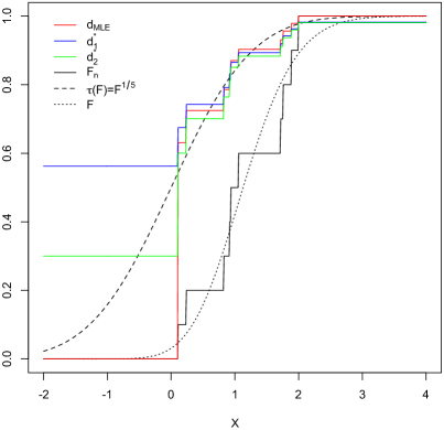
Figure 1: Simulated normal maxima-nomination data ($n=10$, $k=5$).

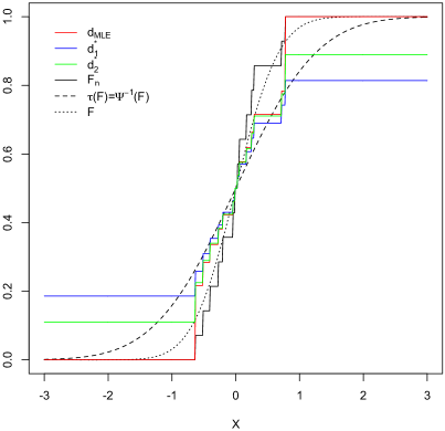
Figure 2: Simulated normal median-nomination data ($n=10$, $k=5$).

This is confirmed visually through a quick inspection of Figure 1 where all considered estimators perform quite well in the right tail based on the maxima nomination sample with $k=5$. Similar behaviour was observed in the cases where $k=3$ and $7$, but results are not reported here. In Figure 1, it is also very interesting to see how working with $d_{2}^{*}$ over $d_{1}^{*}$ leads to improved inference. Indeed, minimizing the integrated distance between $d$ and $\tau(F)$ by weighting that distance with respect to $\tau(F)$ itself gives a much more sensible estimator in the left tail. This is essentially because that left tail plays almost no role when weighting the distance with respect to $F$ (which has a much shorter left tail than $\tau(F)$). As could be expected, the impact of this is particularly important for larger values of $k$. The empirical distribution function $F_{n}$ of the raw data is also shown on all graphs, to help with the comparisons.

$i$	0	1	2	3	4	5
$u_{1,i}^{*}$	0.209	0.291	0.352	0.405	0.453	0.500
$u_{2,i}^{*}$	0.125	0.257	0.332	0.393	0.448	0.500
$u_{MLE,i}$	0.000	0.247	0.327	0.390	0.446	0.500

Table 1: Weights of minimax estimators in the median-nomination sampling case

For median-nomination sampling, we also considered the case where $n=10$ and $k=5$. For all estimators, the values of the weights (obtained from numerical integration, except in the case of the MLE) are provided in Table 1 for $i=0,\ldots,5$. The values that are not displayed in the table can be easily recovered by symmetry of the estimators under the median-nomination sampling (i.e., $u^{*}_{n-i}=1-u^{*}_{i}$). We note that Samawi and Al-Sagheer (2001) suggested to use $F_{n}$ to estimate $\tau(F)$ without modification for values of $t$ such that $\tau(F(t))\simeq 1/2$. Figure 2 suggests that this is reasonable, but that both tails are not captured very well when using this sampling scheme.

5 A case study

Hyperbilirubinemia is a medical condition which commonly affects newborn babies and that arises when the bilirubin levels in the blood exceed 5 mg/dl. Now, bilirubin’s natural pigmentation typically causes a yellowing of the baby’s skin and tissues accompanying hyperbilirubinemia, which is known as jaundice. The level at which the concentration of bilirubin in the blood becomes dangerous is considered to vary between infants, but the effects of bilirubin toxicity can be permanent and include, for instance, developmental delays and hearing loss.

In a study of bilirubin levels in the blood of babies suffering from jaundice staying in the neonatal intensive care unit of five hospitals from Jordan, Samawi and Al-Sagheer (2001) considered data obtained according to a nomination sampling scheme. It is noted that ranking of the level of bilirubin in the blood can be done visually by observing the colour of the face, chest and extremities of babies, as the severity of jaundice is directly related to the concentration of bilirubin in the blood. This fact is quite important as it allows easy ordering of a small number of sampled babies, in terms of bilirubin concentration, without having to actually measure those concentrations by running a blood test, which requires about 30 minutes for completion.

Interest lied mainly in estimating the distribution function of Bilirubin level in the blood of jaundice babies (in mg/dl). Among other things, the authors were interested in recovering the quantile of order 0.95 of Bilirubin level in the blood of jaundice babies. Also, as it is considered that a concentration of 17.65 mg/dl should not be exceeded to avoid any long term repercussions on a baby’s health, they considered the order of the quantile associated with 17.65 as another quantity of interest. Note that both of these quantities are related to the right tail of the underlying distribution, suggesting that a maxima-nomination sampling scheme is appropriate.

We here consider the estimation of the underlying cdf $\tau(F)$ from the $n=14$ maxima listed in Table 4.1 of Samawi and Al-Sagheer (2001). In Figure 3, we have displayed the minimax estimator $d_{2}^{*}$ given in (15), the MLE of $\tau(F)$ given in (16) and the minimax estimator obtained under the balanced loss

$$\int_{0}^{\infty}\big{\{}w(t)\big{(}d_{0}(t)-\tau(F(t))\big{)}^{2}+(1-w(t))\big{(}d(t)-\tau(F(t))\big{)}^{2}\big{\}}d\tau(F(t)),$$

where $\tau(F(t))=\{F(t)\}^{1/5}$, the target estimator $d_{0}$ is the MLE of $\tau(F)$ and the weight function $w$ is such that

$$w(t)=\begin{cases}1/2&\text{if }t<Y_{n}\\ 1&\text{if }t\geq Y_{n}.\end{cases}$$

As in Theorem 4, we obtain the best invariant estimator as follows

$$u_{i}^{*}=\begin{cases}\frac{1}{2}(u_{2,i}^{*}+u_{\text{MLE},i})&\text{for }i=0,1,\ldots,n-1\\ u_{\text{MLE},n}&\text{for }i=n\end{cases},$$

with $u_{2,i}^{*}$ given in (15) with $k=5$. The choice of the weighting function $w$ along with the choice $Y_{0}=0$ (i.e., $a=0$ and $b=\infty$, see Remark 3) forces $d^{*}$ to be a genuine distribution function.

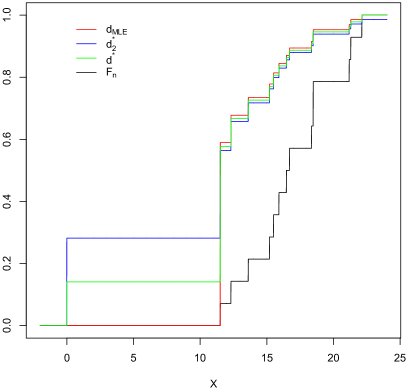
Figure 3: Bilirubin concentrations data ($n=14$, $k=5$).

Figure 3 shows the impact of using a balanced loss approach. Again, the difference between the estimators is most important in the left tail of the estimated distribution. However, this is the most important aspect to consider here as all the considered estimators seem to perform reasonably well in capturing the right tail of $\tau(F)$ in the normal example seen earlier. But, when estimating the left tail of $\tau(F)$, the MLE clearly needs to be improved. Using the suggested balanced loss is one way to accomplish this, while leading to an estimated distribution that is bona fide.

6 Concluding remarks

Our findings relate to the estimation of a continuous distribution function $F$, as well as meaningful functions $\tau(F)$. For the large class of loss functions $L_{\rho,\tau}(d,F)$, as well as weighted versions (Section 2.3), we have obtained best invariant estimators (Section 2.1) and established their minimaxity (Section 2.2) for Hölder continuous $\tau$’s and strict bowl-shaped $\rho$ with a bounded derivative. For identity $\tau$, our minimax result extends previously established results. For non-identity $\tau$, the results are novel and apply as well for the minimaxity of estimators of $\tau(F)$. Many new cases are covered such as integrated $L^{p}$ ($p\geq 1$) losses and integrated ratio losses of the form $\int_{\mathbb{R}}\rho_{0}(\frac{d(t)}{F(t)})\,dF(t)$. We have also remarked upon the (known) fact that best invariant minimax solutions often fail to be genuine distribution functions, and expanded upon corresponding adjustments (Remark 3). In Section 3, we introduced and motivated the use of integrated balanced loss functions which combine the criteria of an integrated distance as above between a decision $d$ and $F$, with the proximity of $d$ with a target estimator $d_{0}$. Moreover, we have shown how the risk analysis of procedures under such an integrated balanced loss relates to a dual risk analysis under an “unbalanced” loss, and we have derived best invariant estimators, minimax estimators, risk comparisons, dominance and inadmissibility results. We believe that the further development of estimating procedures via integrated balanced loss functions is of interest and appealing. For instance, enough flexibility is built in to select a model based or fully parametric target estimator $d_{0}$, assuming for instance a normal distribution function $F$, and obtain compromise efficient procedures such as Theorem 4’s $d_{w}^{*}$.

7 Appendix

7.1 Proof of Theorem 1

Following arguments of Ferguson (1967, Section 4.8), the risk of $d$ in estimating $F$, for any invariant estimator of the form (6) and under the loss (2), may be decomposed as

$$R_{\rho,\tau}(d,F) = E_{F}\big{[}\int_{\mathbb{R}}\rho\big{(}\tau(\sum_{i=0}^{n}u_{i}\mathbb{I}(Y_{i}\leq t<Y_{i+1}))-\tau(F(t))\big{)}\,dF(t)\big{]}$$

$$= E_{F}\big{[}\int_{0}^{1}\rho\big{(}(\sum_{i=0}^{n}\tau(u_{i})\mathbb{I}(Y_{i}\leq F^{-1}(t)<Y_{i+1}))-\tau(t)\big{)}\,dt\big{]}$$

$$= \sum_{i=0}^{n}\int_{0}^{1}\rho(\tau(u_{i})-\tau(t))\,E_{F}(\mathbb{I}(F(Y_{i})\leq t<F(Y_{i+1})))\,dt$$

$$= \sum_{i=0}^{n}\int_{0}^{1}\rho(\tau(u_{i})-\tau(t))\,\binom{n}{i}\,t^{i}\,(1-t)^{n-i}\,dt\,$$ (17)

$$= \frac{1}{n+1}\;\sum_{i=0}^{n}\int_{0}^{1}\rho(\tau(u_{i})-\tau(t))\,f_{T_{i}}(t)\,dt.$$ (18)

With the minimization problem now reducing to minimizing every element of the above sum in (17), the results follow immediately. Also, $\tau(u_{i}^{*})$ minimizes (17) in $\tau(u)$ and hence satisfies the equation $B_{i}(\tau(u_{i}^{*}))=0$, with $B_{i}(\tau(u))=\int_{0}^{1}\rho^{\prime}(\tau(u)-\tau(t))\,\binom{n}{i}\,t^{i}\,(1-t)^{n-i}\,dt\,.$ Since $\rho^{\prime}(\tau(0)-\tau(t))<0$ for all $t\in(0,1)$ given the conditions on $\rho$ and $\tau$, we have $B_{0}(\tau(0))<0$, whence $u_{0}>0$. Similarly, we have $B_{n}(\tau(1))>0$ and $u_{n}<1$. The monotonicity property of the $u^{*}_{i}$’s follows from complete class theorems for monotone procedures such as those provided by Karlin and Rubin (1956) or Brown, Cohen and Strawderman (1976). Indeed, these results apply for families of densities with strict increasing monotone likelihood ratio, such as $\hbox{Bin}(n,p)$ distributions with $p\in[0,1]$, and for the problem of estimating $p$ under strict bowl-shaped loss $L(d,p)$.

7.2 Proof of Lemma 2

Let $\delta,s>0$ and set

$$B_{s}=\{(\textbf{Y},t):|d(\textbf{Y};t)-d_{0}(\textbf{Y};t)|\geq s\}\,.$$

Using Lemma 1, there exists $P_{0}$ (with associated distribution function $F_{0}$) and an estimator $d_{0}\in\mathcal{I}$ such that

$$P_{0}^{n+1}(B_{s})\leq\delta\,.$$ (19)

Now, (i) the triangular inequality, (ii) the boundedness of $\rho^{\prime}$, and (iii) the Hölder continuity assumption enable us to write

$$\big{|}R(d,F_{0})-R(d_{0},F_{0})\big{|} \leq\mathbb{E}_{F_{0}}\left[\int_{\mathbb{R}}\Big{|}\rho(\tau(d(\textbf{Y};t))-\tau(F_{0}(t)))\,-\,\rho(\tau(d_{0}(\textbf{Y};t))-\tau(F_{0}(t)))\Big{|}dF_{0}(t)\right]$$

$$\leq(\sup_{u}\rho^{\prime}(u))\;\mathbb{E}_{F_{0}}\left[\int_{\mathbb{R}}\Big{|}\Big{(}\tau\big{(}d(\textbf{Y};t)\big{)}-\tau\big{(}d_{0}(\textbf{Y};t)\big{)}\Big{)}\Big{|}dF_{0}(t)\right]$$

$$\leq M\,(\sup_{u}\rho^{\prime}(u))\;\mathbb{E}_{F_{0}}\left[\int_{\mathbb{R}}\Big{|}\tau\big{(}d(\textbf{Y};t)\big{)}-\tau\big{(}d_{0}(\textbf{Y};t)\big{)}\Big{|}^{\alpha}\;dF_{0}(t)\right].$$

Making use twice of Jensen’s inequality for concave functions (i.e., $|z|^{\alpha}$ with $\alpha\leq 1$) yields

$$\big{|}R(d,F_{0})-R(d_{0},F_{0})\big{|} \leq M\,(\sup_{u}\rho^{\prime}(u))\left(\mathbb{E}_{F_{0}}\left[\int_{\mathbb{R}}\Big{|}d(\textbf{Y};t)-d_{0}(\textbf{Y};t)\Big{|}dF_{0}(t)\right]\right)^{\alpha},$$ (20)

Using the fact that $|d(\textbf{y};t)-d_{0}(\textbf{y};t)|\leq 1$ for all $t$, we obtain with (19)

$$\mathbb{E}_{F_{0}}\left[\int_{\mathbb{R}}\Big{|}d(\textbf{Y};t)-d_{0}(\textbf{Y};t)\Big{|}dF_{0}(t)\right] =\int_{B_{s}}\big{|}d(\textbf{y};t)-d_{0}(\textbf{y};t)\big{|}dF_{0}^{n+1}(\textbf{y},t)+\int_{B_{s}^{c}}\big{|}d(\textbf{y};t)-d_{0}(\textbf{y};t)\big{|}dF_{0}^{n+1}(\textbf{y},t)$$

$$\leq P_{0}^{n+1}(B_{s})+s\,P_{0}^{n+1}(B_{s}^{c})\leq\delta+s.$$

Finally, substituting this into  (20) and selecting $\delta,s$ such that $\delta+s={\epsilon}^{1/\alpha}\{M(\sup_{u}\rho^{\prime}(u))\}^{-1/\alpha}$, we obtain $|R(d,F_{0})-R(d_{0},F_{0})|\leq\epsilon$, as desired.

7.3 Proof of Theorem 2

We start by noting that Lemma 2 implies that, given $d\in\mathcal{A}$ and $\epsilon>0$, there exists $F_{0}\in\mathcal{F}$ and an invariant estimator $d_{0}\in\mathcal{I}$ such that $\big{|}R_{\tau}(d,F_{0})-R_{\tau}(d_{0},F_{0})\big{|}\leq\epsilon$, implying, in turn, that

$$\sup_{F\in\mathcal{F}}R_{\tau}(d^{*},F)=R_{\tau}(d^{*},F_{0})\leq R_{\tau}(d_{0},F_{0})\leq R_{\tau}(d,F_{0})+\epsilon\leq\sup_{F\in\mathcal{F}}R_{\tau}(d,F)+\epsilon,$$

given that $d^{*}$ is the best invariant estimator under loss (4) with constant risk. Since $d$ and $\epsilon$ are both arbitrary, the stated result follows.

7.4 Proof of Theorem 3

For the best invariant property, proceeding as in the proof of Theorem 1 yields the result. For instance, equation (17) becomes

$$\sum_{i=0}^{n}w_{i}\int_{0}^{1}\rho(\tau(u_{i})-\tau(t))\,\binom{n}{i}\,t^{i}\,(1-t)^{n-i}\,dt\,,$$

and it is clearly seen that the minimization is handled irrespectively of the weights $w_{i}$’s. For the minimaxity, the developments of Section 2.2 go through by simply bounding $w_{n}(\cdot)$ by $1$.

7.5 Complementary developments and proof of Lemma 3

The representations below are used in Lemma 3 and generalize Lemma 1 of Jafari Jozani, Marchand and Parsian (2006). The general context is one of estimating a parameter $\theta$ for the model $Z\sim F_{\theta}$ with loss

$$L_{\omega(\cdot),\delta_{0}}(\delta,\theta)=q(\theta)\,w(z)\,(\delta-\delta_{0})^{2}\,+\,q(\theta)(1-w(z))\,(\delta-\theta)^{2},$$ (21)

where $w(\cdot)\in[0,1]$, $q(\cdot)>0$, and $\delta_{0}$ is a target estimator of $\theta$. Under loss (21), it is easy to check that

$$L_{\omega(\cdot),\delta_{0}}(\delta_{0}+(1-w)g,\theta)=\,q(\theta)\,w(1-w)\,(\delta_{0}-\theta)^{2}\,+\,q(\theta)(1-w)^{2}\,(\delta_{0}+g-\theta)^{2}.$$ (22)

We hence obtain that the risk of the estimator $\delta_{0}(Z)+(1-w(Z))\,g(Z)$ under loss $L_{\omega(\cdot),\delta_{0}}$ is decomposable as

$$R_{\omega(\cdot),\delta_{0}}(\delta_{0}(Z)+(1-w(Z))g(Z),\theta) = E[\,q(\theta)\,w(Z)(1-w(Z))\,(\delta_{0}(Z)-\theta)^{2}]$$

$$+ E[\,q(\theta)(1-w(Z))^{2}\,(\delta_{0}(Z)+g(Z)-\theta)^{2}]\,,$$ (23)

i.e., the sum of the risks of $\delta_{0}(Z)$ and $\delta_{0}(Z)+g(Z)$ with respect to the weighted squared error losses $q(\theta)\,w(z)(1-w(z))(\delta-\theta)^{2}$ and $q(\theta)\,(1-w(z))^{2}\,(\delta-\theta)^{2}$, respectively. Since the former of these risks does not depend on $g(\cdot)$, we have an equivalence between the performance of the estimator $\delta_{0}(Z)+(1-w(Z))\,g(Z)$ under balanced loss (21) and the estimator $\delta_{0}(Z)+\,g(Z)$ under the second of these weighted (and unbalanced) losses. This observation was put forward at the outset of the paper by Jafari Jozani, Marchand and Parsian (2006) for the particular case where $w(\cdot)$ is constant and they pursued with various connections between the balanced loss and unbalanced loss problems as well as applications. A redeployment of their analysis for non-constant weight functions $w(\cdot)$ is available with the above decomposition and of interest. Now, to conclude, expression (22) is used in Lemma 3 with for fixed $(x,t)\in\mathbb{R}^{n+1}$ with $X=Z$, $\theta=\tau(F(t))$, $q(\cdot)=1$ $\delta_{0}=d_{0}(x,t)$, $\delta_{0}+(1-w)g=d_{0}(x,t)+(1-w(x))\,g(x,t)$.

To prove Lemma 3, expanding (10), we have $L_{w,d_{0}}(d_{0}(x,t)+(1-w(x,t)g(x,t),F\,)=$

$$\int_{\mathbb{R}}\{w(x,t)(1-w(x,t))\,[d_{0}(x,t)-\tau(F(t))]^{2}\,+\,(1-w(x,t))^{2}\,[d_{0}(x,t)+g(x,t)-\tau(F(t))]^{2}\,\}\,\,dF(t).$$

The result thus follows at once from (11).

7.6 Proof of Theorem 4

First, observe that $d_{0}^{*}$ is the best invariant procedure under loss $L_{0}$, and thus for risk $R_{H_{2}}$ by virtue of Theorem 3 as $w$ is invariant. Now, under the assumptions on $d_{0}$ and $w$, we see from (12) that the risk $R_{w,d_{0}}$ of invariant estimators is constant with the optimal choice of $g$ arising for $d_{0}+g=d_{0}^{*}$, which gives $d_{w}^{*}=d_{0}+(1-w)(d_{0}^{*}-d_{0})=wd_{0}+(1-w)d_{0}^{*}$.

7.7 Proof of Theorem 5

In representation (12), observe that the first term $R_{H_{1}}(d_{0}(X,\cdot),F)(=C)$ is constant in $F$ since $d_{0}$ is invariant by assumption. Furthermore, Theorem 3 tells us, with the choice $\rho(z)=z^{2}$, that $\sup_{F}\{R_{H_{2}}(d_{0}+g,F)\}\geq\sup_{F}\{R_{H_{2}}(d_{0}^{*},F)\}$ for all $g$. We hence obtain for any estimator $d_{0}+(1-w)\,g\in\cal{A}$:

$$\sup_{F\in\mathcal{F}}\,\{R_{w,d_{0}}(d_{0}+(1-w)g,F\} = C+\sup_{F\in\mathcal{F}}\{R_{H_{2}}(d_{0}+g,F)\}$$

$$\geq C+\sup_{F\in\mathcal{F}}\{R_{H_{2}}(d_{0}^{*},F)\}$$

$$= \sup_{F\in\mathcal{F}}\,\{R_{w,d_{0}}(d_{0}+(1-w)(d_{0}^{*}-d_{0}),F\}$$

$$= \sup_{F\in\mathcal{F}}\,\{R_{w,d_{0}}(d_{w}^{*},F\}\,,$$

which yields the result.

7.8 Proof of Theorem 6

This follows directly from expressing the difference in risk of the two estimators as

$$R_{w,d_{0}}(\alpha\,d_{0}+(1-\alpha)\,d_{0}^{*},F)-R_{w,d_{0}}(\alpha d_{0}+(1-\alpha)d_{1},F)=(1-\alpha)^{2}\{R_{0}(d_{0}^{*},F)-R_{0}(d_{1},F)\}\geq 0,$$

for all $F$, with strict inequality for some.

References

- [1] Aggarwal, O.P. (1955). Some minimax invariant procedures for estimating a cumulative distribution function. Ann. Math. Stat. 26, 450–463.
- [2] Boyles, R.A. and Samaniego, F.J. (1986). Estimating a distribution function based on nomination sampling. Journal of the American Statistical Association 81, 1039–1045.
- [3] Brown, L.D, Cohen, A. and Strawderman, W. E. (1976). A complete class theorem for strict monotone likelihood ratio with applications. Ann. Stat. 4, 712–722.
- [4] Brown, L.D. (1988). Admissibility in discrete and continuous invariant nonparametric estimation problems and in their multinomial analogs. Ann. Stat. 16, 1567–1593.
- [5] Cohen, M.P. and Kuo, L. (1985). The admissibility of the empirical distribution function. Ann. Stat. 13, 262–271.
- [6] Dvoretzky, A., Kiefer, J. and Wolfowitz, J. (1956). Asymptotic minimax character of the sample distribution function and of the classical multinomial estimator. Ann. Math. Stat. 27, 642–669.
- [7] Ferguson, T.S. (1967). Mathematical Statistics: A Decision Theoretic Approach. Academic, New York.
- [8] Friedman, D., Gelman, A. and Phadia, E. (1988). Best invariant estimator of a distribution function under the Kolmogorov-Smirnov loss function. Ann. Stat. 16, 1254–1261.
- [9] Jafari Jozani, M. and Marchand, É. (2007). Minimax estimation of constrained parametric functions for discrete family of distributions. Metrika, 66, 151–160.
- [10] Jafari Jozani, M. and Johnson, B.C. (2012). Randomized nomination sampling for finite populations. Journal of Statistical Planning and Inference 142, 2103–2115.
- [11] Jafari Jozani, M., Marchand, É. and Parsian, A. (2006). On estimation with weighted balanced-type loss function. Statistics & Probability Letters 76, 773–780.
- [12] Karlin, S. and Rubin, H. (1956). The theory of decision procedures for distributions with monotone likelihood ratio. Ann. Math. Stat. 27, 272–299.
- [13] Kvam, P.H. and Samaniego, F.J. (1993). On estimating distribution functions using nomination samples. Journal of the American Statistical Association 88, 1317–1322.
- [14] Mohammadi, L. and van Zwet, W.R. (2002). Minimax invariant estimator of a continuous distribution function under entropy loss. Metrika 56, 31–42.
- [15] Muttlak, H.A. (1997). Median ranked set sampling. Journal of Applied Statistic Science 6, 245–255.
- [16] Ning, J. and Xie, M. (2007). Minimax invariant estimation of a continuous distribution function under LINEX loss. J. Syst. Sci. Complex 20, 119–126.
- [17] Norstrøm, J.G. (1996). The use of precautionary loss function in risk analysis. IEEE Trans. Reliab. 45, 400–403.
- [18] Phadia, E. (1973). Minimax estimation of a cumulative distribution function. Ann. Stat. 1, 1149–1157.
- [19] Samawi, H.M. and Al-Sagheer, O.A.M. (2001). On the estimation of the distribution function using extreme and median ranked set sampling. Biometrical Journal 43, 357–373.
- [20] Samawi, H.M., Ahmed,M. and Abu-Dayyeh,W. (1996). Estimating the population mean using extreme ranked set sampling. Biometrical Journal 38, 577–586.
- [21] Schäbe, H. (1991). Bayes estimates under asymmetric loss. IEEE Trans. Reliab. 40, 63–67.
- [22] Stępień-Baran, A. (2010). Minimax invariant estimator of a continuous distribution function under a general loss function. Metrika, 72, 37–49.
- [23] Wells, M.T. and Tiwari, R.C. (1990). Estimating a distribution function based on minima-nomination sampling. Topics in statistical dependence, IMS Lecture Notes Monogr. Ser. 16, Inst. Math. Statist., Hayward, CA, 471–479.
- [24] Yu, Q. (1989). Methodology for the invariant estimation of a continuous distribution function. Ann. Inst. Stat. Math. 41, 503–520.
- [25] Yu, Q. (1992). Minimax invariant estimator of a continuous distribution function. Ann. Inst. Stat. Math. 44, 729–735.
- [26] Yu, Q. and Phadia, E. (1992). Minimaxity of the best invariant estimator of a distribution function under the Kolmogorov-Smirnov loss. Ann. Stat. 20, 2192–2195.
- [27] Yu, Q. and Chow, M. (1991). Minimaxity of the empirical distribution function in invariant estimation. Ann. Stat. 19, 935–951.
- [28] Willemain, T.R. (1980). Estimating the population median by nomination sampling. Journal of the American Statistical Association 75, 908–911.